Article

On the Classification–Causal Tradeoff in Neural Network Propensity Score Estimation

1
School of Nursing, Texas Tech University Health Sciences Center, Lubbock, TX 79430, USA
2
Department of Educational Psychology, Leadership, and Counseling, College of Education, Texas Tech University, Lubbock, TX 79409, USA
*
Author to whom correspondence should be addressed.
Stats 2026, 9(2), 37; https://doi.org/10.3390/stats9020037
Submission received: 20 February 2026 / Revised: 24 March 2026 / Accepted: 30 March 2026 / Published: 31 March 2026

Abstract

Observational studies serve as a vital alternative to randomized experiments but are highly susceptible to selection bias. Propensity score (PS) methods address this by balancing covariates between groups. Although including all relevant covariates is theoretically ideal, high dimensionality often destabilizes traditional estimation models. This study evaluates the efficacy of deep neural networks (DNN) and convolutional neural networks (CNN) for PS estimation compared to traditional logistic regression (LR), leveraging their capacity to handle complex nonlinear relationships and interactions. Using a Monte Carlo simulation across 36 conditions, model performance was evaluated based on bias and imbalance reduction. Results indicate that DNNs and CNNs significantly outperform LR. Specifically, while LR increased outcome bias by 17% and reduced covariate imbalance by only 5%, DNNs and CNNs reduced outcome bias by 13% and 16%, respectively, while decreasing covariate imbalance by 18% and 21%. We conclude that despite requiring specialized computational resources, neural networks offer substantial advantages for high-dimensional PS estimation. However, their reliable application necessitates stability-aware training and proper error rate thresholds to prevent probability degeneracy.

1. Introduction

1.1. Causal Inference in Observational Research

Establishing causal effects is a fundamental objective when evaluating the impact of treatments or interventions. While randomized controlled trials (RCTs) represent the gold standard for causal inference by eliminating selection bias through random assignment, they are frequently unfeasible due to ethical constraints or prohibitive costs [1]. In such scenarios, researchers rely on observational data from surveys, medical charts, or censuses [2]. Because participants in observational studies are not randomly assigned, baseline differences between groups—known as selection bias—often confound the relationship between treatment and outcome [3]. To establish causality, it is imperative to ensure that comparison groups are comparable at baseline.

1.2. Propensity Score Methods

Propensity score methods (PSMs) are the primary statistical framework used to address this lack of comparability by balancing covariates between groups [4,5,6]. The propensity score (PS) is defined as the conditional probability of a subject receiving treatment based on their observed covariates [7]. These scores are utilized to match, weight, or stratify subjects, thereby mimicking the properties of a randomized experiment [8]. To satisfy the “strongly ignorable treatment assignment” assumption [7,8,9], researchers must include all relevant covariates in the PS estimation model. However, this necessity frequently produces high-dimensional datasets that challenge the capacities of traditional statistical models [10,11].

1.3. Traditional and Emerging Estimation Architectures

Generalized linear modeling (GLM) is the conventional framework for PS estimation. The most established method, logistic regression (LR), uses available covariates to predict binary treatment status [12]. Logistic mixed-effects models further extend this by accounting for clustered data [12,13]. While LR effectively models simple relationships, its parametric nature restricts its utility in high-dimensional settings because it assumes covariates are linear and additive on a log-odds scale.
The increasing complexity of observational data demands flexible estimation methods capable of handling numerous variables without rigid distributional assumptions. Machine learning techniques excel in these environments by effectively managing complex, nonlinear interactions [14,15]. To address the limitations of LR, we propose using deep neural networks (DNNs) and convolutional neural networks (CNNs), which offer enhanced flexibility and accuracy for large-scale datasets [16,17,18,19].
A DNN features multiple hidden layers where neurons learn complex data patterns [17,20], using backpropagation and gradient descent to minimize predictive errors without rigid distributional assumptions [17,20]. Conversely, CNNs perform automated feature extraction via convolutional and pooling layers, which facilitates dimensionality reduction for complex data [20]. By maintaining input topology, CNNs capture localized dependency structures [18,19,20]. For PS estimation, CNNs process restructured two-dimensional covariate data to estimate the probability of treatment.
Recent studies in causal machine learning often emphasize predictive accuracy as the primary objective for flexible models [14,15]. In contrast, our proposed Classification–Causal Tradeoff framework highlights the potential divergence between predictive performance and causal validity. Models aggressively optimized for classification accuracy may fail to minimize bias in treatment effect estimation. By examining this tension, our framework illustrates how machine learning optimization goals directly influence the stability of causal inference.

1.4. Purpose of the Study

While LR remains effective for simple datasets, high-dimensional data structures necessitate advanced machine learning alternatives [10,11,21]. Although tree-based methods like random forests and classification and regression trees (CART) have been successfully employed to enhance PS weighting [11,22], empirical investigations into DNNs and CNNs remain scarce. Initial evidence suggests these architectures can yield superior cross-entropy compared to traditional boosted modeling [12,16].
A central challenge addressed in this work is the classification–causal tradeoff: aggressively optimizing neural networks for predictive accuracy may push propensity scores toward 0 or 1. This violates the positivity assumption, yielding unstable inverse probability weights and inflated variance in causal effect estimation [23]. Through a comprehensive Monte Carlo simulation, this study evaluates the performance of DNNs and CNNs in reducing selection bias and covariate imbalance. By implementing a stability-aware training framework—such as restricting epochs—we provide an evidence-based approach for selecting optimal PS estimation methods. While tree-based ensemble methods (e.g., Random Forest, Gradient Boosting) are effective [24], they operate on different structural principles than neural architectures and fall outside the specific scope of this study.
The remainder of this manuscript is organized as follows. Section 2 details the materials, data generation, and the proposed stability-aware training framework. Section 3 presents the simulation results. Section 4 and Section 5 discuss practical implications, methodological recommendations, and future research directions.

2. Materials and Methods

2.1. Population Model and Data Generation

The simulation generated datasets featuring 10,000 subjects assigned to treatment and control groups. This sample size was selected to reflect large-scale observational datasets common in contemporary causal inference research. To systematically evaluate the models across varying degrees of confounding and multicollinearity, correlation parameters were set to represent small (0.1), medium (0.3), and large (0.5) associations based on Cohen’s established guidelines [25].
A zero correlation between TG and Y indicates the random assignment of subjects, as no systematic intervention occurs in the assignment process. In contrast, a nonzero correlation between TG and Y indicates nonrandom assignment because subjects with a higher Y value are more likely to be assigned to the treatment group (i.e., selection bias).
An outcome variable Y was generated following a standard normal distribution (M = 0, SD = 1). A temporary group (TG) variable was constructed to correlate with Y at levels of 0, 0.1, 0.3, or 0.5. Subjects were sorted descendingly by their TG value. The top 1000, 2500, or 4000 subjects were designated as the treatment group (T = 1), representing treatment sizes (TS) of 10%, 25%, or 40%, respectively. The remaining subjects formed the control group (T = 0). A zero correlation between TG and Y simulates random assignment, while a nonzero correlation simulates nonrandom assignment driven by selection bias.
Table 1 illustrates an example of nonrandom assignment with a TG-Y correlation of 0.5. Subjects were sorted and assigned to the treatment group (T = 1) based on their TG ranking. Because TG and Y are positively correlated, subjects in the treatment group inherently exhibited higher Y values. For instance, at a 25% treatment size (TS), the mean Y for the treatment group was 0.69, compared to just −0.01 for the control group.
Continuous covariates X1–X18 were generated following a standard normal distribution (M = 0, SD = 1) and had a correlation of 0.1, 0.3, or 0.5 with other covariates (rXX). The covariate-outcome correlations (rXY) were set to 0.1 (small) for X1–X6; 0.3 (medium) for X7–X12; and 0.5 (large) for X13–X18. Concurrently, the covariate-group correlations (rXT (rXT represents the correlation between covariates Xs and the temporary group variable TG. Because TG was employed for the purpose of generating the final group variable T, we chose to use the term rXT, instead of rXTG, for simplicity)) were systematically structured across these sets: (i) 0.1 for X1, X7, and X13; (ii) 0.2 for X2, X8, and X14; (iii) 0.3 for X3, X9, and X15; (iv) 0.4 for X4, X10, and X16; (v) 0.5 for X5, X11, and X17; and (vi) 0.6 for X6, X12, and X18.
Crossing these parameters yielded a 3 × 3 × 4 factorial design consisting of 36 simulation conditions. For each condition, 200 datasets were generated, totaling 7200 datasets and 720 million subjects. Propensity scores were estimated using (a) DNN and (b) CNN through Python 3.8, TensorFlow 2.4.1, and Keras 2.4.3 in Visual Studio 2019, and (c) LR through R [26] in RStudio 1.3.1056 [27].

2.2. Theoretical Framework: Classification–Causal Tradeoff

In classification tasks, the objective is to minimize predictive loss, typically cross-entropy:
L ( θ ) = E T log e ^ X + 1 T log 1 e ^ X .
Here, T denotes the treatment indicator and e ^ ( X ) represents the estimated propensity score given covariates X. In standard machine learning classification problems, minimizing this cross-entropy loss improves the model’s ability to correctly predict treatment assignment. In causal inference, however, the PS is used to construct inverse probability weights rather than merely predict treatment status. Minimizing classification loss too aggressively drives predicted probabilities toward 0 or 1, producing unstable weights. Valid weighting-based inference requires the positivity condition:
0 < e ( X ) < 1
To formalize this empirically, we define:
ε = min 1 i n min e ^ X i , 1 e ^ X i .
When ε→0, estimated probabilities approach degeneracy (0 or 1), leading to instability in weighting estimators.
Proposition 1 (Weight Explosion). For stabilized IPTW weights,
w i = T i π e ^ X i + 1 T i 1 π 1 e ^ X i .
it holds that
max i   w i min π , 1 π ε .
Thus, as ε→0, extreme weights diverge.
Proposition 2 (Variance Inflation). The IPTW estimator
τ ^ = 1 n i = 1 n T i Y i e ^ X i 1 T i Y i 1 e ^ X i .
has variance that increases as
E 1 e ^ X + E 1 1 e ^ X .
increases. Hence, minimizing classification loss may increase variance when probabilities collapse toward 0 or 1. The minimum value ε reflects the proximity of estimated propensity scores to the boundaries of the unit interval. When ε becomes small, some estimated probabilities approach 0 or 1, leading to extremely large inverse probability weights. Consequently, smaller ε values are associated with greater instability and variance inflation in weighting-based causal estimators. In practice, models optimized primarily for classification accuracy may produce highly confident predictions, which reduces ε and increases the risk of weight explosion.
Theorem (Classification–Causal Tradeoff). Minimizing cross-entropy loss does not guarantee optimal causal estimation performance. Under separable conditions, aggressive optimization may induce near-degenerate propensity scores, thereby violating empirical positivity and inflating variance.

2.3. Stability-Aware Training and Hyperparameters

Stability-Aware Training Strategy. Given this tradeoff, we implement a stability-preserving training rule:
ε   ε 0 ,
for a predefined lower bound ε 0 > 0 . Rather than optimizing classification accuracy to convergence, training is terminated once the loss remains non-degenerate and predicted probabilities remain bounded away from 0 and 1.
In our simulation settings, this stability condition was typically satisfied around 20 epochs, which prevented complete separation while maintaining adequate predictive accuracy.
Hyperparameters. In this study, as an optimizer, the stochastic gradient descent (SGD) algorithm was chosen for the DNN and CNN models with a learning rate of 0.01. Following Heaton’s [28] recommendations, two hidden layers were used. The number of neurons in the hidden layers was determined based on the following guidelines: (i) between the number of neurons in the input and output layers, (ii) 2/3 of the total number of neurons, and (iii) less than twice the number of neurons in the input layer. For the DNN, the first hidden layer contained 189 neurons, equal to the input layer, and the second hidden layer had 94 neurons, half the number in the first hidden layer. For CNN, the first hidden layer included 64 neurons, and the second hidden layer had 32 neurons.
To prevent overfitting and to ensure a proper loss rate (see Accuracy and Loss Rate above), the network models were forced to stop at 20 epochs even though minimizing loss required more epochs. Since the models were not complex and given the low likelihood of overfitting, we did not drop any connections (dropout rate = 0). Three batch sizes were used: 100 (small), 1000 (medium), and 2000 (large). The ReLU activation function was applied, and the HE initializer was used to select the initial biases and weights in the network models. The HE initializer is considered optimal for ReLU activation functions [20,29].

2.4. Model Architectures

Deep Neural Network. The DNN model consisted of one input layer, two hidden layers, and one output layer. The layers were arranged as a fully connected neural network, with all neurons in each layer connected to all neurons in the subsequent layer (see Figure 1). The input layer included 189 neurons, corresponding to all covariates (X1X18), their interaction terms (X1×2, X1×3, …, X17×18), and squared terms (X12, X22, …, X182). The first and second hidden layers featured 189 and 94 neurons, respectively. The output layer comprised a single neuron, representing the conditional probability of subjects being treated (i.e., propensity score).
Convolutional Neural Network. In this study, the data structure for the CNN model differed from that of the DNN model, as the CNN requires multidimensional data. Thus, the original data, consisting of covariates ( X 1 X 18 ) and their squared terms ( X 1 2 , X 2 2 , , X 18 2 ), were transformed into two-dimensional (36 × 36) data. Furthermore, all values in the transformed data were scaled within the range 0 to 255, as digital images are typically represented by numbers from 0 to 255, regardless of whether the image is grayscale (one channel: 2D) or color (more than two channels: RGB and alpha).
Although CNNs were originally developed for spatially structured data such as images, recent studies have demonstrated that they can also be applied to high-dimensional tabular data by transforming feature vectors into structured matrix representations. In such approaches, the two-dimensional representation does not impose spatial meaning but instead provides a structured input format that enables convolutional filters to detect localized dependency patterns among variables. This idea has been explored in several studies that convert tabular features into image-like representations in order to leverage convolutional architectures for feature extraction by preserving feature similarities in a 2D space [18,19]. In high-dimensional PS estimation problems involving nonlinear transformations and interactions among covariates, such structured representations allow CNN filters to capture local dependency structures while benefiting from parameter sharing across neighboring elements. Consequently, the CNN architecture can act as a form of implicit regularization, helping to model complex treatment assignment mechanisms while mitigating overfitting relative to fully connected neural networks.
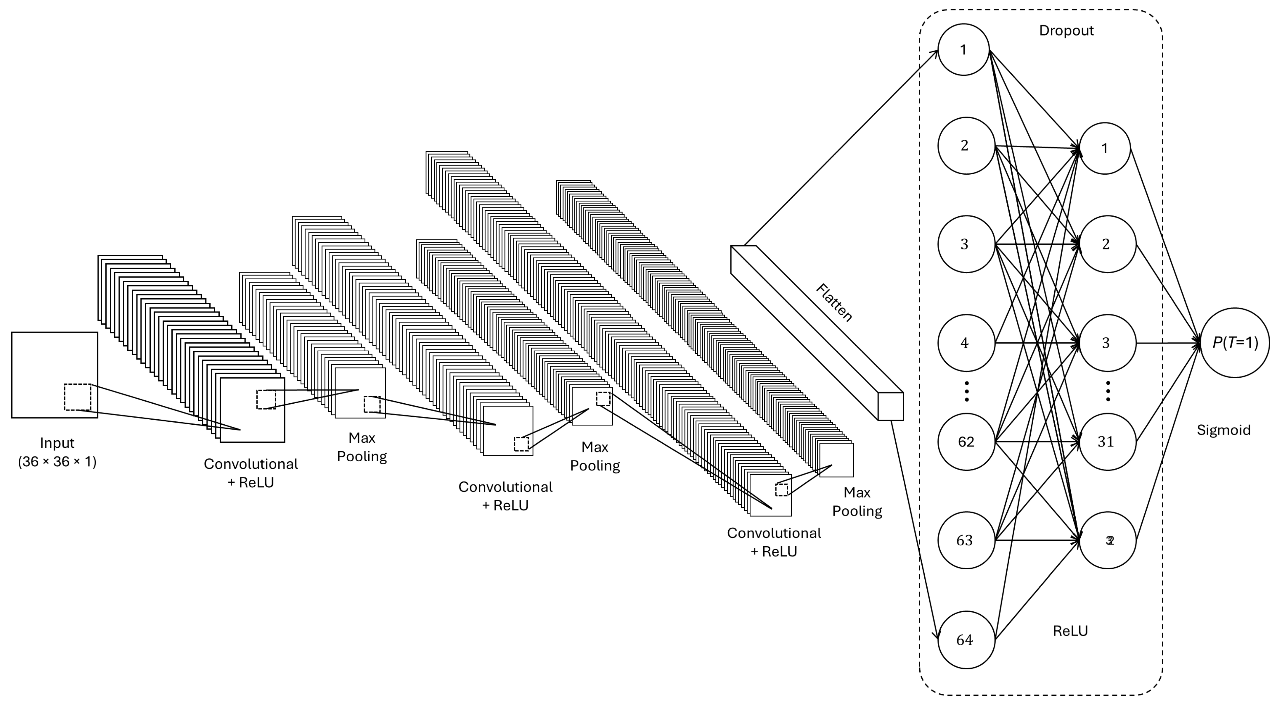
The CNN model had a three-layer structure with convolutional layers, ReLU activation functions, 2D max-pooling layers, and a flatten layer to extract features from the two-dimensional (36 × 36) data of covariates and their squared terms. The convolutional layers were designed with 32 filters and a 3 × 3 kernel size to extract relevant features from the data. The 2D max-pooling layers followed the convolutional layers to downsample the features, and the flatten layer converted the extracted features into a single linear vector for input into a fully connected neural network at the end of the model structure (Figure 2).
Logistic Regression. LR was conducted using the ‘glm’ function in R [26]. The LR model included all covariates (X1–X18), their interaction terms (X1X2, X1X3, …, X17X18), and squared terms (X12, X22, …, X182). The ‘predict’ R function produced an estimated PS for each subject from the fitted LR model.

2.5. Propensity Score Weighting and Analysis

To evaluate the performance of the three estimation methods (DNN, CNN, LR), we examined bias reduction in the outcomes (Ys) and covariates (Xs). Two weighting methods were chosen for the PS analysis: (1) weighted by odds and (2) weighted by IPTW. To obtain the weights using the odds method, treated subjects (T = 1) were given a weight of 1, while untreated subjects were given a weight of their PS converted to the odds scale ( P S 1 P S ) [4,8]. For weighting by the IPTW method, treated subjects received E ( P S ) P S and untreated subjects received E ( 1 P S ) 1 P S as their stabilized weights [3,30,31]. This resulted in each subject having six weights (odds and stabilized IPTW for each of the three estimation methods).
We fitted linear regression models, with Y or covariates (X1 to X18) as the outcome and T as the predictor. The models were fitted with weights (with residuals weighted by the six weights described above) and again without weights. For subjects who are untreated (T = 0), the outcome Y of the linear model is expressed as Y T = 0 = β 0 + ε . For those who receive the treatment (T = 1), Y is expressed as Y T = 1 = β 0 + β 1 + ε . Thus, the difference between YT=1 and YT=0 equals β 1 , which is the regression coefficient representing the treatment effect:
Y ( o r   X i ) = β 0 + β 1 T + ε , where   i   ranges   from   1   to   18 .
In particular, β 1 in the unweighted models it represents the treatment effect under the presence of selection bias, whereas in the weighted models, it represents the treatment effect when the bias has been accounted for by weighting. In this study, reductions in bias (in the outcome and covariates) by using the PSM were calculated as the difference in the estimated treatment effect ( β 1 ^ ) from the unweighted vs. weighted models.

3. Results

3.1. Accuracy and Loss Rate (For DNN and CNN)

Table 2 summarizes mean classification accuracy and cross-entropy loss for DNN and CNN under 5-fold cross-validation. Although predictive accuracy varied slightly across rTY and batch size conditions, both models maintained comparable accuracy levels (approximately 0.85–0.87). From a causal inference perspective, these values are not interpreted as indicators of optimal classification performance, but rather as evidence that models did not approach perfect separation.
More importantly, cross-entropy loss remained in the range of approximately 0.33–0.37 across all conditions due to the stability-aware training strategy. This non-degenerate loss level indicates that predicted propensity scores did not collapse toward 0 or 1. Maintaining such bounded probabilities is essential to preserve empirical positivity and prevent extreme inverse probability weights. Therefore, the reported accuracy and loss rates should be understood as reflecting controlled optimization rather than maximal predictive fitting.

3.2. Bias Reduction

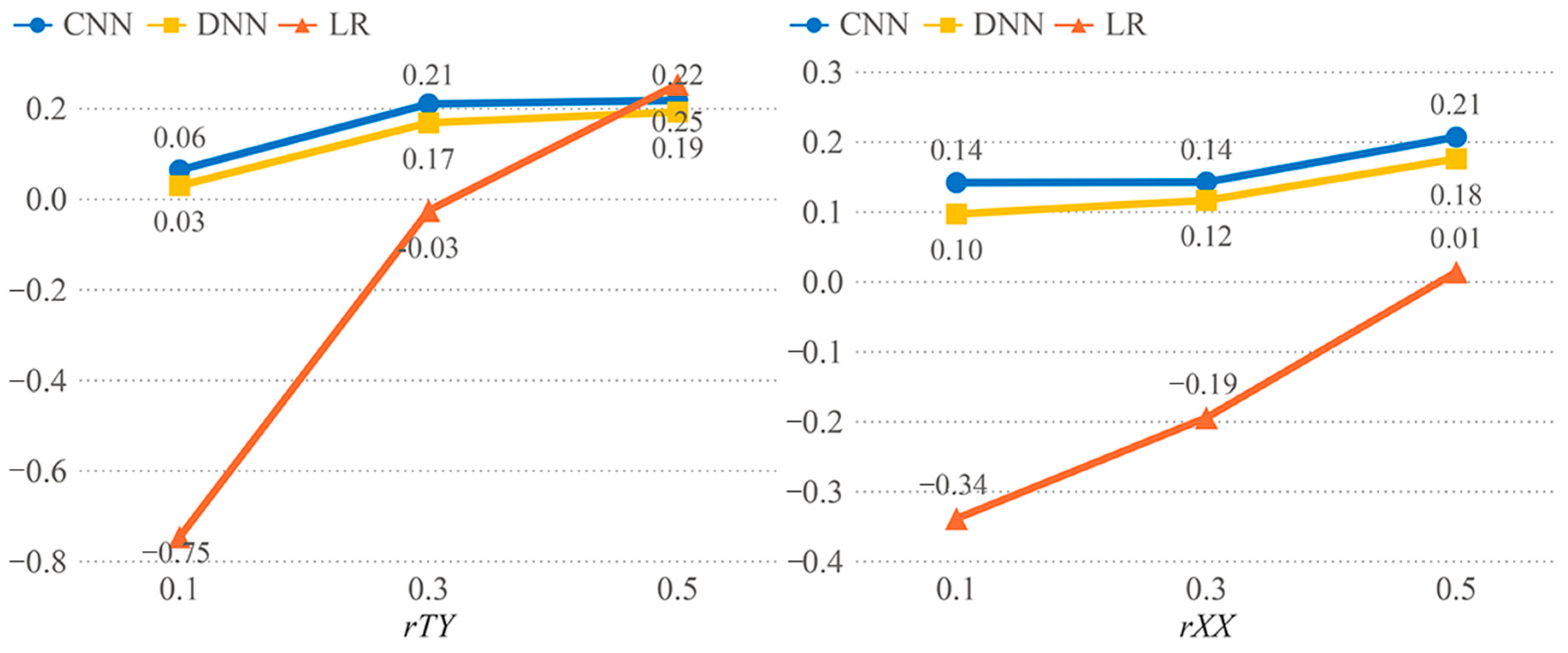
Figure 3 illustrates bias reduction in the outcome variable across estimation methods. All three methods demonstrated greater bias reduction as rTY and rXX increased, reflecting stronger treatment–outcome associations. Under the stability-aware training framework, both DNN and CNN achieved substantial bias reduction relative to LR.
While CNN exhibited slightly higher average bias reduction than DNN across most conditions, pairwise comparisons indicated no statistically significant difference between the two neural network approaches. In contrast, LR frequently exhibited minimal bias reduction or even bias amplification, particularly under lower rTY levels. In some simulation settings, LR produced larger bias than the proposed models. This phenomenon can arise when the treatment assignment mechanism involves nonlinear relationships or interactions among covariates that are not adequately captured by the linear logit specification of LR. In such cases, misspecification of the PS model may lead to insufficient covariate balance after weighting, resulting in increased bias in treatment effect estimation [8,32]. Additionally, LR may generate extreme propensity score estimates in finite samples, particularly under strong covariate separation, which can lead to unstable inverse probability weights and increased variance in the resulting causal estimator.
These results suggest that flexible nonlinear estimators, when trained under stability constraints, can better capture treatment assignment mechanisms without inducing degeneracy in estimated propensity scores.
Table 3 provides numerical summaries of the bias reduction results across estimation methods. The table reports the numerical values corresponding to the patterns shown in Figure 3.

3.3. Imbalance Reduction

Table 4 presents imbalance reduction in covariates across methods. Significant differences were observed among estimation approaches. Both DNN and CNN consistently reduced covariate imbalance more effectively than LR across rTY and rXX conditions.
CNN exhibited marginally greater average imbalance reduction compared with DNN. However, this difference should be interpreted within the broader stability framework: architectural constraints in CNN may moderate effective model complexity, thereby influencing how nonlinear treatment assignment mechanisms are captured under empirical positivity constraints.
LR, in contrast, demonstrated limited capacity to adjust imbalance under more complex correlation structures, highlighting the limitations of strictly parametric models in high-dimensional settings.
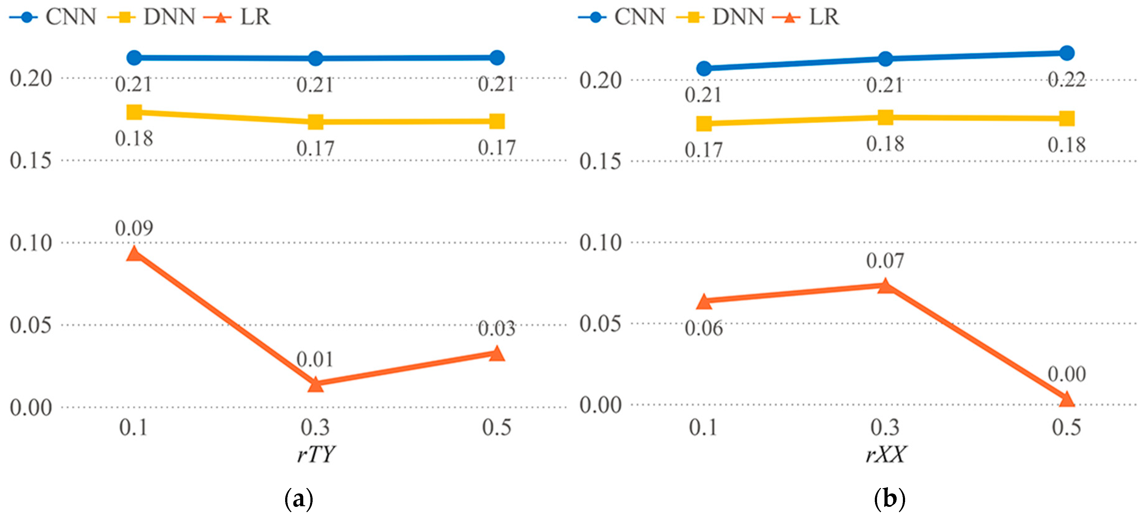
Figure 4 visually illustrates imbalance reduction across varying levels of rTY and rXX. The graphical patterns provide an intuitive comparison of the imbalance reduction achieved by each method across correlation conditions. Neural network estimators demonstrated relatively stable imbalance reduction across scenarios, whereas LR exhibited greater sensitivity to correlation strength.
Overall, the visual patterns in Figure 4 complement the numerical results reported in Table 4 and highlight the improved balance preservation achieved by the neural network–based estimators.
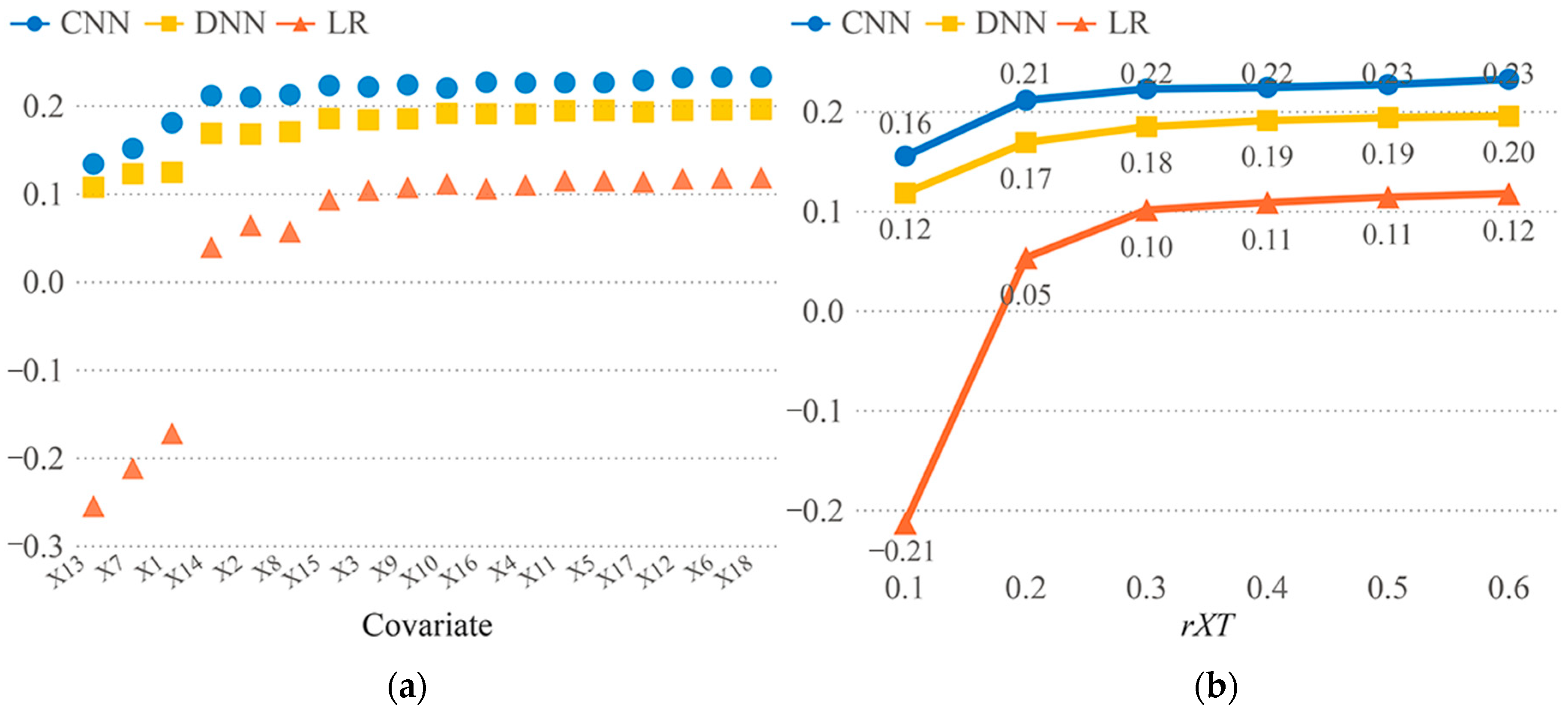
Figure 5 provides a more granular view of imbalance reduction across individual covariates and varying levels of rXT. Across estimation methods, imbalance reduction increased as the strength of the covariate–treatment association intensified. This pattern reflects the intuitive relationship that stronger associations provide clearer signals for PS adjustment.
Importantly, both DNN and CNN maintained consistent imbalance reduction even for covariates with weaker rXT, whereas LR exhibited limited correction under such conditions. These findings suggest that flexible nonlinear estimators are better equipped to capture heterogeneous assignment structures across covariates, particularly when combined with stability-aware training to preserve overlap.

4. Discussion

The advent of neural networks has brought about groundbreaking developments in various areas by their unparalleled accuracy levels, and these advances suggest that neural networks can be an innovative and promising methodology for estimating PS as well. For instance, the effective use of DNNs and CNNs as PS estimators holds significant potential for diverse domains, including healthcare, marketing, and social sciences. Researchers and practitioners might be able to leverage these techniques to enhance causal inference, treatment effect estimations, and policy evaluations in their respective areas. Furthermore, exploring potential synergies when DNN, CNN, and other machine learning approaches are used together (such as ensemble methods and transfer learning) might be able to improve the performance of PS estimation. Such integration may result in more accurate estimations, ultimately elevating the quality of causal inferences from observational data.
However, it is vital to recognize that solely focusing on enhancing network performance in terms of accuracy may not consistently produce applicable PSs. The optimal hyperparameters for obtaining the proper PS depend on the shapes of the data, such as dimensionality, the number of cases, and inherent patterns. Given that actual datasets vary in shape, this remains a challenging and intricate task. Consequently, empirical trials serve as the only means of discovering these optimal configurations. The insights gleaned from the current study endorse implementing a restricted number of epochs within neural networks instead of adjusting batch sizes. This approach aims to balance maintaining ideal loss rates and achieving acceptable classification accuracy. By following these recommendations, researchers can obtain proper propensity scores.
Although we found that DNN exhibited slightly lower performance compared to CNN, it still holds merit for cost-effectiveness. Among the three estimation methods examined, DNN achieved the quickest estimation time, taking only 2.1 min for a single simulation condition, which was three times faster than LR and 15 times faster than CNN (see Table 5). Although the DNN took a considerably shorter time to estimate PS, its performance was only slightly below that of the CNN. Consequently, DNNs may be well suited for scenarios where rapid PS estimation is necessary. However, we also found that to obtain an applicable PS while maintaining an appropriate loss rate and high accuracy, an intricate network structure is not always a prerequisite. In this study, we demonstrated the effectiveness of a DNN with just two hidden layers and a limited number of neurons, which still yielded satisfactory performance.
Within the proposed classification–causal tradeoff framework, the role of convolutional neural networks should be interpreted beyond conventional predictive superiority. Although CNNs are traditionally designed for spatially structured data, their architectural features—such as parameter sharing, localized connectivity, and hierarchical feature extraction—can be viewed as imposing structured constraints on model complexity.
In high-dimensional PS settings that include interaction and nonlinear transformations, reshaping covariates into a structured matrix representation enables convolutional filters to capture localized dependency patterns among covariates and their higher-order terms. More importantly, such architectural constraints may function as implicit regularization, limiting the tendency of the model to drive predicted probabilities toward degeneracy under aggressive loss minimization.
From the perspective of weighting-based causal estimation, the value of CNN lies not solely in improved bias reduction, but in how its structural properties interact with the empirical positivity requirement. By moderating effective model flexibility, CNN may reduce the probability of extreme fitted values and mitigate weight instability within the stability-aware training regime.
However, this structural regularization comes at the cost of increased computational complexity, as convolutional operations and multidimensional transformations require greater processing time compared to fully connected architectures.
Recent research has increasingly explored the use of flexible machine learning methods for PS estimation and causal effect estimation in settings with complex treatment assignment mechanisms. Approaches such as Bayesian additive regression trees, causal forests, and high-dimensional covariate balancing methods have demonstrated improved performance in modeling nonlinear relationships and high-dimensional confounding structures compared with traditional parametric models [33,34,35]. These studies highlight the potential advantages of flexible nonparametric learners for estimating treatment assignment mechanisms in observational data.
Previous research has emphasized that PS models should not be evaluated solely by their ability to predict treatment assignments. Instead, the fundamental role of the PS is to function as a balancing score that equalizes covariate distributions between treatment groups [4,7]. Consequently, improvements in predictive accuracy do not necessarily translate into improved covariate balance or more reliable causal effect estimation.
In the context of machine learning–based PS estimation, Lee et al. [22] similarly argued that the quality of a PS model should be assessed by the degree to which it achieves covariate balance rather than by its classification performance. Moreover, the presence of extreme predicted probabilities can threaten the positivity assumption and lead to unstable inverse probability weights, potentially inflating variance in causal estimators [23].
Taken together, these perspectives highlight a fundamental distinction between predictive optimization and causal validity. The classification–causal tradeoff observed in the present study is consistent with this literature: models optimized solely for classification may produce near-degenerate propensity scores, whereas stability-aware training helps preserve overlap and maintain reliable weighting-based causal inference. In particular, the simulation results demonstrate that neural network estimators trained under stability-aware constraints achieve improved bias and imbalance reduction while avoiding the degeneracy issues often associated with highly flexible models.
This study employed the TensorFlow and Keras frameworks, which are advanced machine learning and artificial intelligence libraries, along with a Python interface for seamless integration and execution. TensorFlow, an end-to-end open-source machine learning platform developed by the Google Brain team, facilitates the creation and training of complex neural networks. Additionally, Keras, an open-source library for building high-level neural networks, simplifies the process of defining and training various machine learning models.
Apart from TensorFlow and Keras, other prominent statistical tools, such as SAS, MATLAB, and R, also offer robust machine-learning frameworks and libraries. These versatile platforms allow researchers to effectively conduct and broaden their studies on PSMs by using advanced neural network architectures without encountering significant challenges. They also enable researchers to explore innovative methodologies for PS estimation, harnessing the full potential of machine learning techniques in the realm of causal inference and observational studies. By leveraging the capabilities of these advanced tools, it is possible to optimize PS analysis and make substantial strides in the understanding and application of machine learning in various fields.

5. Conclusions

The present study investigated neural-network-based PS estimation through the lens of a classification–causal tradeoff. While deep learning models are typically optimized to minimize predictive loss, we demonstrate that excessive classification optimality may undermine the stability requirements of weighting-based causal inference. In particular, near-degenerate propensity scores can induce extreme inverse probability weights and variance inflation, even when predictive accuracy appears high.
By formalizing this tension, we introduced a stability-aware training framework that preserves empirical positivity while retaining the flexibility of neural networks. Within this framework, both DNN and CNN achieved improved bias and imbalance reduction compared to LR under controlled stability conditions. Importantly, our findings suggest that optimal PS estimation is not equivalent to optimal classification performance; instead, stability constraints must be explicitly incorporated into the training process.
The contribution of this work lies not merely in performance comparison but in clarifying the structural relationship between predictive optimization and causal validity. Neural-network-based PS estimators should therefore be trained with explicit consideration of overlap preservation and weight stability, rather than solely minimizing classification loss.
Several limitations warrant consideration. First, the theoretical results presented here provide structural insight into weight instability under probability degeneracy, but do not constitute a full asymptotic characterization of neural-network-based PS estimators. Future research may formally establish convergence properties and finite-sample bounds under stability constraints.
Second, although our Monte Carlo design encompassed a wide range of correlation structures and sample sizes, simulated data cannot fully capture the distributional complexity of real-world observational settings. Because the primary scope of this study was to mathematically isolate the classification–causal tradeoff under strictly controlled conditions, a pilot application using real data falls outside the boundaries of this initial investigation. Following these successful simulations, our immediate direction for future research is to conduct a dedicated follow-up study that illustrates this stability-aware framework using empirical observational datasets.
Third, the stability-aware criterion employed in this study was implemented via early stopping. While this approach effectively prevented degeneracy in our simulations, alternative mechanisms—such as probability clipping, entropy regularization, or explicit overlap constraints—may offer theoretically grounded improvements. Comparative analysis of such stabilization strategies remains an important direction for future research.
Finally, the architectural role of convolutional neural networks was interpreted here as structured regularization under high-dimensional transformations. A formal characterization of how convolutional constraints influence effective model complexity and positivity preservation constitutes an open methodological question.

Author Contributions

Conceptualization, S.K., J.L. and K.J.; methodology, S.K., J.L. and K.J.; formal analysis, S.K.; investigation, J.L. and K.J.; validation, J.L. and K.J.; writing—original draft preparation, S.K.; writing—review and editing, S.K., J.L. and K.J.; supervision, J.L. and K.J.; project administration, J.L. All authors have read and agreed to the published version of the manuscript.

Funding

This research received no external funding.

Institutional Review Board Statement

Not applicable.

Informed Consent Statement

Not applicable.

Data Availability Statement

The source code used to generate the simulated datasets and execute the estimation models is available in the project repository at https://github.com/jaehoonlee-ttu/ps-dnn_cnn.git (accessed on 19 February 2026).

Conflicts of Interest

The authors declare no conflicts of interest.

References

  1. Johnson, R.B.; Christensen, L.B. Educational Research: Quantitative, Qualitative, and Mixed Approaches, 6th ed.; SAGE Publications: Thousand Oaks, CA, USA, 2016. [Google Scholar]
  2. Guo, S.; Fraser, M.W. Propensity Score Analysis: Statistical Methods and Applications, 2nd ed.; SAGE Publications: Thousand Oaks, CA, USA, 2014. [Google Scholar]
  3. Austin, P.C.; Stuart, E.A. Moving towards best practice when using inverse probability of treatment weighting (IPTW) using the propensity score to estimate causal treatment effects in observational studies. Stat. Med. 2015, 34, 3661–3679. [Google Scholar] [CrossRef] [Scilit]
  4. Austin, P.C. An introduction to propensity score methods for reducing the effects of confounding in observational studies. Multivar. Behav. Res. 2011, 46, 399–424. [Google Scholar] [CrossRef] [Scilit] [PubMed]
  5. Austin, P.C. A comparison of 12 algorithms for matching on the propensity score. Stat. Med. 2013, 33, 1057–1069. [Google Scholar] [CrossRef] [Scilit]
  6. Thoemmes, F.J.; Kim, E.S. A systematic review of propensity score methods in the social sciences. Multivar. Behav. Res. 2011, 46, 90–118. [Google Scholar] [CrossRef] [Scilit]
  7. Rosenbaum, P.R.; Rubin, D.B. The central role of the propensity score in observational studies for causal effects. Biometrika 1983, 70, 41–55. [Google Scholar] [CrossRef]
  8. Lee, J.; Little, T.D. A practical guide to propensity score analysis for applied clinical research. Behav. Res. Ther. 2017, 98, 76–90. [Google Scholar] [CrossRef] [Scilit]
  9. Rosenbaum, P.R. Observational Studies; Springer: Berlin/Heidelberg, Germany, 1995. [Google Scholar]
  10. Breiman, L. Statistical Modeling: The Two Cultures. Stat. Sci. 2001, 16, 199–215. [Google Scholar] [CrossRef] [Scilit]
  11. Westreich, D.; Lessler, J.; Funk, M.J. Propensity score estimation: Neural networks, support vector machines, decision trees (CART), and meta-classifiers as alternatives to logistic regression. J. Clin. Epidemiol. 2010, 63, 826–833. [Google Scholar] [CrossRef] [Scilit]
  12. McCaffrey, D.F.; Ridgeway, G.; Morral, A.R. Propensity score estimation with boosted regression for evaluating causal effects in observational studies. Psychol. Methods 2004, 9, 403–425. [Google Scholar] [CrossRef] [Scilit] [PubMed]
  13. Zuur, A.F.; Ieno, E.N.; Walker, N.; Saveliev, A.A.; Smith, G. Mixed Effects Models and Extensions in Ecology with R; Springer: Berlin/Heidelberg, Germany, 2009. [Google Scholar] [CrossRef] [Scilit]
  14. Brand, J.E.; Zhou, X.; Xie, Y. Recent Developments in Causal Inference and Machine Learning. Annu. Rev. Sociol. 2023, 49, 81–110. [Google Scholar] [CrossRef] [Scilit] [PubMed]
  15. Guo, Y.; Strauss, V.Y.; Català, M.; Jödicke, A.M.; Khalid, S.; Prieto-Alhambra, D. Machine learning methods for propensity and disease risk score estimation in high-dimensional data: A plasmode simulation and real-world data cohort analysis. Front. Pharmacol. 2024, 15, 1395707. [Google Scholar] [CrossRef] [Scilit] [PubMed]
  16. Collier, Z.A.; Leite, W.L.; Zhang, H. Estimating propensity scores using neural networks and traditional methods: A comparative simulation study. Commun. Stat. Simul. Comput. 2022, 51, 5780–5795. [Google Scholar] [CrossRef] [Scilit]
  17. Borisov, V.; Leemann, T.; Seßler, K.; Haug, J.; Pawelczyk, M.; Kasneci, G. Deep neural networks and tabular data: A survey. IEEE Trans. Neural Netw. Learn. Syst. 2022, 35, 7499–7519. [Google Scholar] [CrossRef] [Scilit]
  18. Zhu, Y.; Brettin, T.; Xia, F.; Partin, A.; Shukla, M.; Yoo, H.; Evrard, Y.A.; Doroshow, J.H.; Stevens, R. Converting tabular data into images for deep learning with convolutional neural networks. Sci. Rep. 2021, 11, 11325. [Google Scholar] [CrossRef] [Scilit]
  19. Sharma, A.; Vans, E.; Shigemizu, D.; Boroevich, K.A.; Tsunoda, T. DeepInsight: A methodology to transform non-image data to an image for convolution neural network architecture. Sci. Rep. 2019, 9, 11399. [Google Scholar] [CrossRef] [Scilit]
  20. Goodfellow, I.; Bengio, Y.; Courville, A. Deep Learning; MIT Press: Cambridge, MA, USA, 2016; Available online: https://www.deeplearningbook.org/ (accessed on 13 December 2018).
  21. Farrell, M.H.; Liang, T.; Misra, S. Deep neural networks for estimation and inference. Econometrica 2021, 89, 181–213. [Google Scholar] [CrossRef] [Scilit]
  22. Lee, B.R.; Lessler, J.; Stuart, E.A. Improving propensity score weighting using machine learning. Stat. Med. 2010, 29, 337–346. [Google Scholar] [CrossRef] [Scilit]
  23. D’Amour, A.; Ding, P.; Feller, A.; Lei, L.; Sekhon, J. Overlap in observational studies with high-dimensional covariates. J. Econom. 2021, 221, 644–654. [Google Scholar] [CrossRef] [Scilit]
  24. Couronné, R.; Probst, P.; Boulesteix, A. Random forest versus logistic regression: A large-scale benchmark experiment. BMC Bioinform. 2018, 19, 270. [Google Scholar] [CrossRef] [Scilit]
  25. Cohen, J. Statistical Power Analysis for the Behavioral Sciences, 2nd ed.; Routledge: New York, NY, USA, 1977. [Google Scholar] [CrossRef] [Scilit]
  26. R Core Team. R: A Language and Environment for Statistical Computing; R Foundation for Statistical Computing: Vienna, Austria, 2021; Available online: https://www.R-project.org/ (accessed on 13 April 2023).
  27. RStudio Team. RStudio: Integrated Development for R; RStudio (PBC): Boston, MA, USA, 2020; Available online: http://www.rstudio.com/ (accessed on 28 July 2022).
  28. Heaton, J. Introduction to Neural Networks with Java, 2nd ed.; Heaton Research: St. Louis, MO, USA, 2008. [Google Scholar]
  29. He, K.; Zhang, X.; Ren, S.; Sun, J. Delving deep into rectifiers: Surpassing human-level performance on ImageNet classification. In Proceedings of the IEEE International Conference on Computer Vision, Santiago, Chile, 7–13 December 2015; pp. 1026–1034. [Google Scholar] [CrossRef] [Scilit]
  30. Hirano, K.; Imbens, G.W.; Ridder, G. Efficient estimation of average treatment effects using the estimated propensity score. Econometrica 2003, 71, 1161–1189. [Google Scholar] [CrossRef] [Scilit]
  31. Robins, J.M.; Hernán, M.N.; Brumback, B. Marginal structural models and causal inference in epidemiology. Epidemiology 2000, 11, 550–560. [Google Scholar] [CrossRef] [Scilit]
  32. Levy, J.M.; O’Malley, A.J. Don’t dismiss logistic regression: The case for sensible extraction of interactions in the era of machine learning. BMC Med. Res. Methodol. 2020, 20, 171. [Google Scholar] [CrossRef] [Scilit]
  33. Hill, J. Bayesian nonparametric modeling for causal inference. J. Comput. Graph. Stat. 2011, 20, 217–240. [Google Scholar] [CrossRef] [Scilit]
  34. Imai, K.; Ratkovic, M. Covariate balancing propensity score. J. R. Stat. Soc. Ser. B 2014, 76, 243–263. [Google Scholar] [CrossRef] [Scilit]
  35. Wager, S.; Athey, S. Estimation and inference of heterogeneous treatment effects using random forests. J. Am. Stat. Assoc. 2018, 113, 1228–1242. [Google Scholar] [CrossRef] [Scilit]
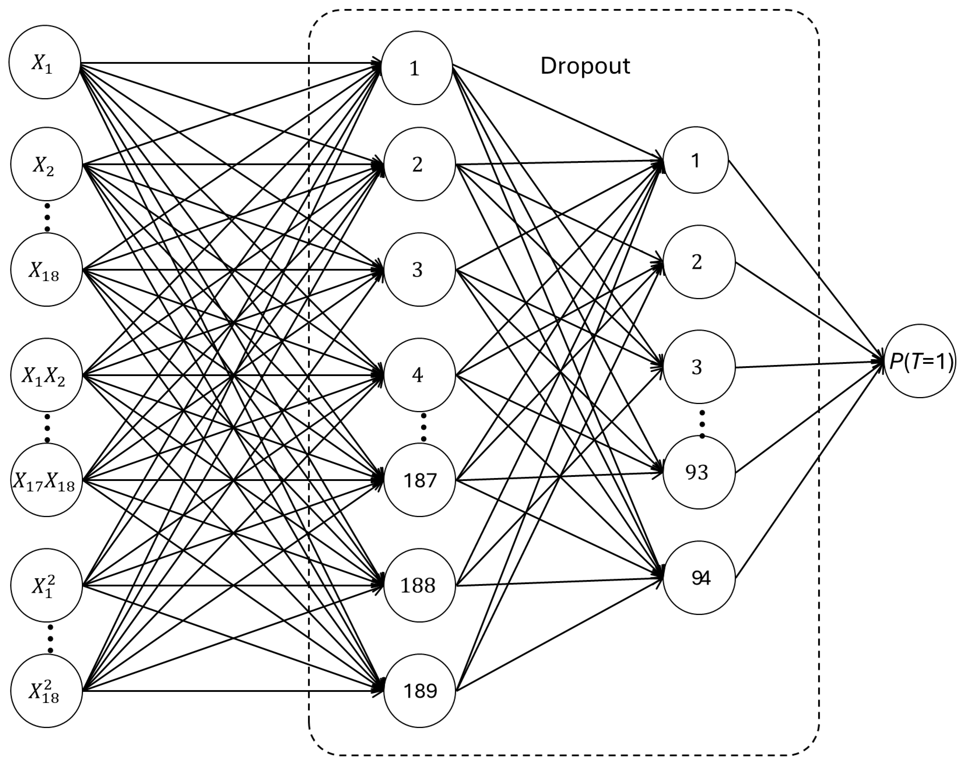
Figure 1. Structure of the Deep Neural Network (DNN) used for Propensity Score Estimation. Note. The network consists of an input layer containing covariates, interaction terms, and squared terms, followed by two fully connected hidden layers with dropout regularization and a single output neuron producing the estimated propensity score.
Stats 09 00037 g001
Figure 2. Structure of the Convolutional Neural Network (CNN) used for Propensity Score Estimation. Note. Covariates and their squared terms were reshaped into a two-dimensional matrix and processed through convolutional layers with ReLU activation and max-pooling operations, followed by a flatten layer and a fully connected layer producing the estimated propensity score.
Stats 09 00037 g002
Figure 3. Bias Reduction in the Estimated Treatment Effect for DNN, CNN, and LR.
Stats 09 00037 g003
Figure 4. Reduction in Covariate Imbalance across Simulated Conditions of rTY (a) and rXX (b).
Stats 09 00037 g004
Figure 5. Imbalance Reduction across Individual Covariates (a) and rXT (b).
Stats 09 00037 g005
Table 1. Example of Nonrandom Assignment of Subjects.
Subject IDTGYT
52.501.551
212.173.661
61.801.871
52–1.83–1.910
40–1.86–0.440
65–2.00–1.200
Table 2. Average Accuracy and Loss Rate for Training and Validation of the DNN and CNN.
Batch SizerTYDNNCNN
TrainingValidationTrainingValidation
Acc.LossAcc.LossAcc.LossAcc.Loss
1000.10.8630.3460.8630.3460.8620.3470.8590.351
0.30.8680.3370.8680.3380.8670.3390.8640.343
0.50.8740.3330.8740.3320.8730.3340.8700.338
10000.10.8580.3600.8580.3600.8520.3630.8520.363
0.30.8620.3540.8610.3540.8550.3570.8530.358
0.50.8680.3500.8680.3490.8600.3530.8590.355
20000.10.8550.3700.8540.3700.8440.3740.8450.373
0.30.8580.3650.8570.3650.8470.3690.8480.368
0.50.8640.3610.8640.3610.8510.3660.8520.366
Table 3. Comparison of Bias Reduction in Outcome.
CNN (C)DNN (D)LR (L)Overall DifferencePairwise Comparison
MSEMSEMSEFpCohen’s fC vs. DC vs. LD vs. L
Overall0.160.010.130.01–0.170.0747.67<0.0010.500.363<0.001<0.001
rXX
0.10.140.010.100.02–0.340.1238.08<0.0010.790.503<0.001<0.001
0.30.140.010.120.02–0.190.179.94<0.0010.400.884<0.001<0.001
0.50.210.000.180.010.010.0815.08<0.0010.500.431<0.001<0.001
rTY
0.10.060.010.030.02–0.750.12106.00<0.0011.310.680<0.001<0.001
0.30.210.000.170.01–0.030.0542.69<0.0010.830.059<0.001<0.001
0.50.220.000.190.010.250.053.150.0460.230.3160.3460.044
Table 4. Comparison of Imbalance Reduction in Covariates.
CNN (C)DNN (D)LR (L)Overall DifferencePairwise Comparison
MSEMSEMSEFpCohen’s fC vs. DC vs. LD vs. L
Overall0.210.000.180.000.050.01714.60<0.0010.46<0.001<0.001<0.001
rTY
  0.10.210.000.180.000.090.02113.30<0.0010.32<0.001<0.001<0.001
  0.30.210.000.170.000.010.01342.20<0.0010.55<0.001 <0.001<0.001
  0.50.210.000.170.000.030.01318.50<0.0010.53<0.001<0.001<0.001
rXX
  0.10.210.000.170.000.060.02136.30<0.0010.35<0.001<0.001<0.001
  0.30.210.000.180.000.070.01182.80<0.0010.40<0.001<0.001<0.001
  0.50.220.000.180.000.000.01543.80<0.0010.69<0.001<0.001<0.001
Covariate
  X10.180.000.120.01–0.170.05100.20<0.0010.730.004<0.001<0.001
  X20.210.000.170.010.060.0345.02<0.0010.49<0.001<0.001<0.001
  X30.220.000.180.010.100.0338.25<0.0010.45<0.001<0.001<0.001
  X40.230.000.190.010.110.0339.66<0.0010.46<0.001<0.001<0.001
  X50.230.000.160.000.110.0338.98<0.0010.46<0.001<0.001<0.001
  X60.230.000.200.000.120.0341.71<0.0010.47<0.001<0.001<0.001
  X70.150.000.120.01–0.210.05100.40<0.0010.73<0.001<0.001<0.001
  X80.210.000.170.010.060.0349.60<0.0010.51<0.001<0.001<0.001
  X90.220.000.180.010.110.0338.65<0.0010.45<0.001<0.001<0.001
  X100.220.000.190.010.110.0236.09<0.0010.44<0.001<0.001<0.001
  X110.230.000.190.000.110.0339.06<0.0010.46 0.001<0.001<0.001
  X120.230.000.190.000.120.0342.05<0.0010.47<0.001<0.001<0.001
  X130.130.010.110.01–0.260.0683.76<0.0010.670.45<0.001<0.001
  X140.210.000.170.010.040.0358.99<0.0010.56<0.001<0.001<0.001
  X150.220.000.190.010.090.0347.59<0.0010.50<0.001<0.001<0.001
  X160.230.000.190.010.110.0344.09<0.0010.48<0.001<0.001<0.001
  X170.230.000.190.000.110.0340.54<0.0010.47<0.001<0.001<0.001
  X180.230.000.200.000.120.0342.38<0.0010.48<0.001<0.001<0.001
Table 5. Summary of Performance Comparison.
LRDNNCNN
Bias reduction in outcome17% increased13% decreased16% decreased
Imbalance reduction in covariates5% decreased18% decreased21% decreased
Time (in minutes)6.52.131.8
Disclaimer/Publisher’s Note: The statements, opinions and data contained in all publications are solely those of the individual author(s) and contributor(s) and not of MDPI and/or the editor(s). MDPI and/or the editor(s) disclaim responsibility for any injury to people or property resulting from any ideas, methods, instructions or products referred to in the content.