Synthetic Hydrograph Estimation for Ungauged Basins: Exploring the Role of Statistical Distributions

Abstract

The use of probability distribution functions in deriving synthetic hydrographs has become a robust method for modeling the response of watersheds to precipitation events. This approach leverages statistical distributions to capture the temporal structure of runoff processes, providing a flexible framework for estimating peak discharge, time to peak, and hydrograph shape. The present study explores the application of various probability distributions in constructing synthetic hydrographs. The research evaluates parameter estimation techniques, analyzing their influence on hydrograph accuracy. The results highlight the strengths and limitations of each distribution in capturing key hydrological characteristics, offering insights into the suitability of certain probability distribution functions under varying watershed conditions. The study concludes that the approach based on the Cadariu rational function enhances the adaptability and precision of synthetic hydrograph models, thereby supporting flood forecasting and watershed management.

1. Introduction

The synthetic hydrograph (SH) is a fundamental tool in hydrology, used to model the response of a watershed to a unit input of excess precipitation over a specified duration. It plays an essential role in hydraulic analysis for the design and verification of hydraulic structures, such as protective levees, dams, and other flood defense works. The SH contributes to determining the maximum water volume that must be retained or released, being crucial for establishing reservoir dimensions and attenuation basin capacities. It is used in hydraulic modeling of flood wave propagation, serving as input data for hydrodynamic models that simulate its downstream movement, assessing the wave’s velocity and height in various river cross-sections. Additionally, it plays an important role in the sizing and verification of levees, allowing the assessment of their stability and height, including the analysis of internal erosion and infiltration effects during extreme events.

Unlike observed hydrographs, which are derived directly from recorded rainfall–runoff events, SHs are constructed using empirical or analytical methods, making them highly adaptable in ungauged or poorly monitored watersheds.

The construction of synthetic flood hydrographs often relies on using different functions for the rising and falling limbs. Sokolovski’s model [1], for example, employs exponential functions, providing a specific formula for calculating discharge on the rising limb. Other models, such as the Reitz–Kreps model [2], combine exponential and sinusoidal functions—applying a sinusoidal expression on the rising limb and an exponential relation on the falling limb. Srebrenovic [3] introduced an approach that uses a composite power–sine function for the rising limb and a power-type function for the falling limb.

In recent years, probabilistic approaches have gained prominence in the development of SHs, offering a more flexible and statistically robust framework for capturing the inherent variability and uncertainty of hydrological processes. Probability distribution functions (PDFs) are particularly useful in this context, as they describe the likelihood of various flow magnitudes occurring over time, allowing for a more realistic representation of runoff dynamics, for the entire shape of the hydrograph.

Commonly employed PDFs in SH derivation include the gamma distribution [4,5,6], Weibull distribution [7], log-normal distribution [8], beta distribution [4,7,9], Fréchet distribution [10], three-parameter Kumaraswamy distribution [11], two-parameter Pareto distribution [11], two-parameter inverse Gaussian distribution [11], two-parameter inverse gamma distribution [11], also known as the Pearson V distribution, Dagum distribution [12], log-logistic distribution [13], also known as generalized logistics distribution, etc.

The gamma distribution is often favored for its ability to capture the skewed nature of runoff hydrographs, while the Weibull distribution is useful for modeling time to peak and recession curves, especially in extreme flow conditions. These distributions help in defining the shape and scale parameters of the hydrograph, thus enabling hydrologists to simulate peak flow rates, time to peak, and recession curves with greater accuracy. For example, in a study conducted on a small mountainous watershed [14], the gamma and beta distributions provided a superior fit for the rising limb of the hydrograph, accurately predicting peak discharge times. Meanwhile, the Weibull distribution was effective in characterizing the recession limb, reflecting the gradual drainage of runoff over time.

The use of PDFs not only enhances the predictive capabilities of the SH but also facilitates the estimation of design flows for flood risk assessment, irrigation planning, and other water resource management practices. Furthermore, probabilistic modeling allows for the quantification of uncertainty in hydrograph predictions, supporting more informed decision-making processes.

When using these probability distribution functions, it is crucial to ensure that all defining conditions of a synthetic flood hydrograph are met. These conditions include the critical time (time to peak, $T_c$), the total duration of the hydrograph ($T_t$), the peak discharge ($Q_{p\%}$), and the shape coefficient of the synthetic flood hydrograph ($\gamma$), which represents the ratio between the flood volume ($W_{SH}={\displaystyle \underset{0}{\overset{T_t}{\int }}Q\left(t\right)\cdot dt}$) and the equivalent volume of the rectangle circumscribed to the flood wave ($W_R=T_t\cdot Q_{p\%}$).

A particularly important aspect is the skewness of these synthetic floods, as the rising limb is typically steeper than the recession limb. This skewness must be accurately captured by the chosen PDF, since it plays a key role in the design of hydraulic structures, such as spillways, flood outlets, and in establishing operational rules for reservoirs. Failure to account for this skewness could lead to underestimations of peak flows or miscalculations of recession times, both of which are critical for flood risk management and infrastructure resilience.

In Romania, it is a standard and common practice in hydrology to establish, based on observed floods at hydrometric stations, regional and zonal values for the characteristic parameters of hydrographs. These are average elements of the typical singular flood waves. To establish these average values, series of observed floods at hydrometric stations are used, selecting significant events (usually annual maximum floods or floods caused by rainfall with certain exceedance probabilities). For each flood, the rise time (the time from the beginning of the flow increase to the peak) and the total time (usually defined as the duration until the flow returns close to its initial value) are determined. The observed values are correlated with the morphometric characteristics of the basins: area (A), main river length (L), average slope (S), etc., constructing empirical relationships where the coefficients are adjusted based on multiple regression applied to monitored basins. The obtained values are grouped by hydrological zones or regions with similar characteristics (geology, climate, land use, etc.). The models are tested by comparing synthetic hydrographs with observed ones, adjusting the coefficients to minimize errors.

For ungauged basins, it provides an indirect but well-founded method to estimate the hydrograph parameters. In hydrological modeling, it helps create synthetic hydrographs, useful for the design of hydraulic structures. For frequency analysis, it allows the simulation of hydrographs corresponding to different return periods, even without detailed local data.

Thus, with this information, the unit hydrograph is created, which needs to be scaled by the peak flow corresponding to the desired annual exceedance probability. For ungauged basins, the peak flow is estimated through a similarity analysis with adjacent gauged basins, where a flood frequency analysis (FFA) of recorded peak flow series is conducted to determine the extreme event values associated with the relevant annual exceedance probabilities (p%).

To reduce uncertainties in estimating these peak flows, the frequency analysis should adopt a holistic approach, considering statistical distributions and parameter estimation methods. Given the well-documented advantages highlighted in numerous studies and analyses, it is recommended that Romania adopt the L-moments method—a robust and stable technique, resistant to the influence of outliers and variability in data series lengths [15,16,17,18,19].

Thus, considering these regional hydrological approaches for determining the parameters of synthetic flood waves (critical time, total time, flood volume, and flood shape coefficient), the question arises: What is the most suitable and easily applicable formula/relation/probability distribution density function for constructing the synthetic hydrograph, while ensuring all these parameter values are respected?

In this context, the manuscript analyzes several of the most commonly used probability density functions: the Weibull distribution, the triangular distribution, Bazin’s relation, and Vladimirescu’s relation. Furthermore, the manuscript presents a function initially proposed by engineer Radu Cadariu [20], which represents an elegant solution (a three-parameter rational function) both mathematically and statistically, offering significant advantages over classical approaches (as evidenced by the case study results presented in the paper). Unfortunately, this function has been “forgotten”—whether intentionally or not—in the hydrological technical literature of Romania.

By integrating statistical methods into hydrological modeling, this research seeks to contribute to the development of more reliable and adaptable tools for deriving synthetic hydrographs.

In general, these regionally determined parameters are provided in hydrological studies, where they form the basis for constructing the unit hydrograph and the hydrograph corresponding to the peak flow (associated with the desired annual exceedance probability). This is essential for performing hydraulic modeling to identify floodplain boundaries and flood-prone areas, helping to establish the necessary structural and non-structural flood protection measures for various objectives. These parameters also play a crucial role in analyses of the probabilities and failure mechanisms of protective structures, such as levees, particularly through the piping failure mechanism, where the flood volume is critically important.

Thus, this manuscript presents an analysis aimed at identifying the best model for constructing the peak hydrograph, based on data from locations where these regionally determined parameters were provided.

As innovative elements, approximate relations with errors < 1% are presented regarding the estimation of the parameters of the Cadariu and Bazin functions, innovative elements that help determine the parameters and facilitate the ease of use and application of these functions in representing the synthetic hydrograph. In general (valid for all statistical distributions that can be used to represent the synthetic unit flood hydrographs), the estimation of the function parameters results from solving the following conditions: ${\displaystyle \frac{dF(t)}{dt}}=0$, $F\left(T_c\right)=1$, and ${\displaystyle \frac{{\displaystyle \underset{0}{\overset{T_t}{\int }}F\left(t\right)\cdot dt}}{T_t}}=\gamma$.

2. Methods

This section presents the expressions of the probability density functions of the analyzed distributions and the conditions required for parameter estimation.

2.1. Cadariu’s Formula

The function was first proposed in 1979 by Radu Cadariu. The model is based on a dimensionless analytical function of the form [20]:

$$Q^{\ast }={\displaystyle \frac{t^{\ast }\cdot \left(T_t-t\right)}{A\cdot t^{\ast }+B^{\ast }+C}},$$

(1)

where:

$Q^{\ast }$ represents the ratio between a current discharge value $Q$ and the maximum discharge value, $Q_{\max }$.

$t^{\ast }$ represents the ratio between a current value of time, $t$, and the value of the growth duration, $T_c$.

$T^{\ast }$ represents the ratio between a current value of time, $T$, and the value of the growth duration, $T_c$.

$A,B,C$ represent the dimensionless parameters that determine the shape of the hydrograph.

Thus, taking these into account, the characteristic elements of the flood hydrograph are the following [20]:

$$Q_{\max }^{\ast }={\displaystyle \frac{Q_{\max }}{Q_{\max }}}=1,$$

(2)

$$T_c^{\ast }={\displaystyle \frac{T_c}{T_c}}=1,$$

(3)

$$T^{\ast }={\displaystyle \frac{T}{T_c}}\ge 2,$$

(4)

$$\gamma ={\displaystyle \frac{W^{\ast }}{T^{\ast }}},$$

(5)

where $W^{\ast }$ represents the dimensionless volume of the flood wave.

To determine the three parameters ($A$, $B$, and $C$), the following 3 conditions must be met [20]:

(1)

The function passes through the coordinate point: $t^{\ast }=T_c^{\ast }=1$, $Q^{\ast }=Q_m^{\ast }=1$.

From this condition, it follows that the parameter $B$ has the expression:

$$B=T^{\ast }-2\cdot \left(A+1\right).$$

(6)

(2)

Let the abscissa of the maximum point of the function, $Q^{\ast }$, be $t^{\ast }=T_c^{\ast }=1$. From this condition, the expression of the parameter $C$ results:

$$C={\displaystyle \frac{B+A\cdot T^{\ast }}{T^{\ast }-2}}={\displaystyle \frac{T^{\ast }-2\cdot \left(A+1\right)+A\cdot T^{\ast }}{T^{\ast }-2}}=A+1.$$

(7)

(3)

The integral of the function, $Q^{\ast }\left(t^{\ast }\right)$, must be equal to 1:

$$W^{\ast }={\displaystyle \underset{0}{\overset{T^{\ast }}{\int }}{Q}^{\ast }\left(t^{\ast }\right)\cdot d{t}^{\ast }}=\gamma \cdot T^{\ast }.$$

(8)

Substituting the expressions of the parameters $B$ and $C$ into the expression of the last condition, a nonlinear equation with a single unknown parameter, namely, $A$ [20], results:

$$\begin{array}{l}{W}^{\ast }={\displaystyle \frac{\left(A+1\right)\cdot \left(T^{\ast }-2\right)}{A^2}}\cdot \ln \left(T^{\ast }-1\right)-{\displaystyle \frac{T^{\ast }}{A}}+\\ {\displaystyle \frac{\left(A+1\right)\cdot \left[2\cdot A\cdot \left(T^{\ast }-1\right)-{\left(T^{\ast }-2\right)}^2\right]}{A^2\cdot \sqrt{4\cdot A\cdot \left(T^{\ast }-1\right)-{\left(T^{\ast }-2\right)}^2}}}\cdot \left[arctg\left({\displaystyle \frac{2\cdot A\cdot \left(T^{\ast }-1\right)+T^{\ast }-2}{\sqrt{4\cdot A\cdot \left(T^{\ast }-1\right)-{\left(T^{\ast }-2\right)}^2}}}\right)-arctg\left({\displaystyle \frac{T^{\ast }-2\cdot \left(A+1\right)}{\sqrt{4\cdot A\cdot \left(T^{\ast }-1\right)-{\left(T^{\ast }-2\right)}^2}}}\right)\right]\end{array}$$

(9)

With the parameters $A$, $B$, and $C$ determined, the final function representing the synthetic hydrograph is the following [20]:

$$Q\left(t\right)=Q_0+(Q_{p\%}-Q_0)\cdot {\displaystyle \frac{t\cdot \left(T_t-t\right)}{A\cdot t^2+B\cdot T_c\cdot t+C\cdot T_c^2}},$$

(10)

where $Q_0$ represents the base flow (for simplicity, it is chosen to be zero, considering that the flood wave is analyzed exclusively).

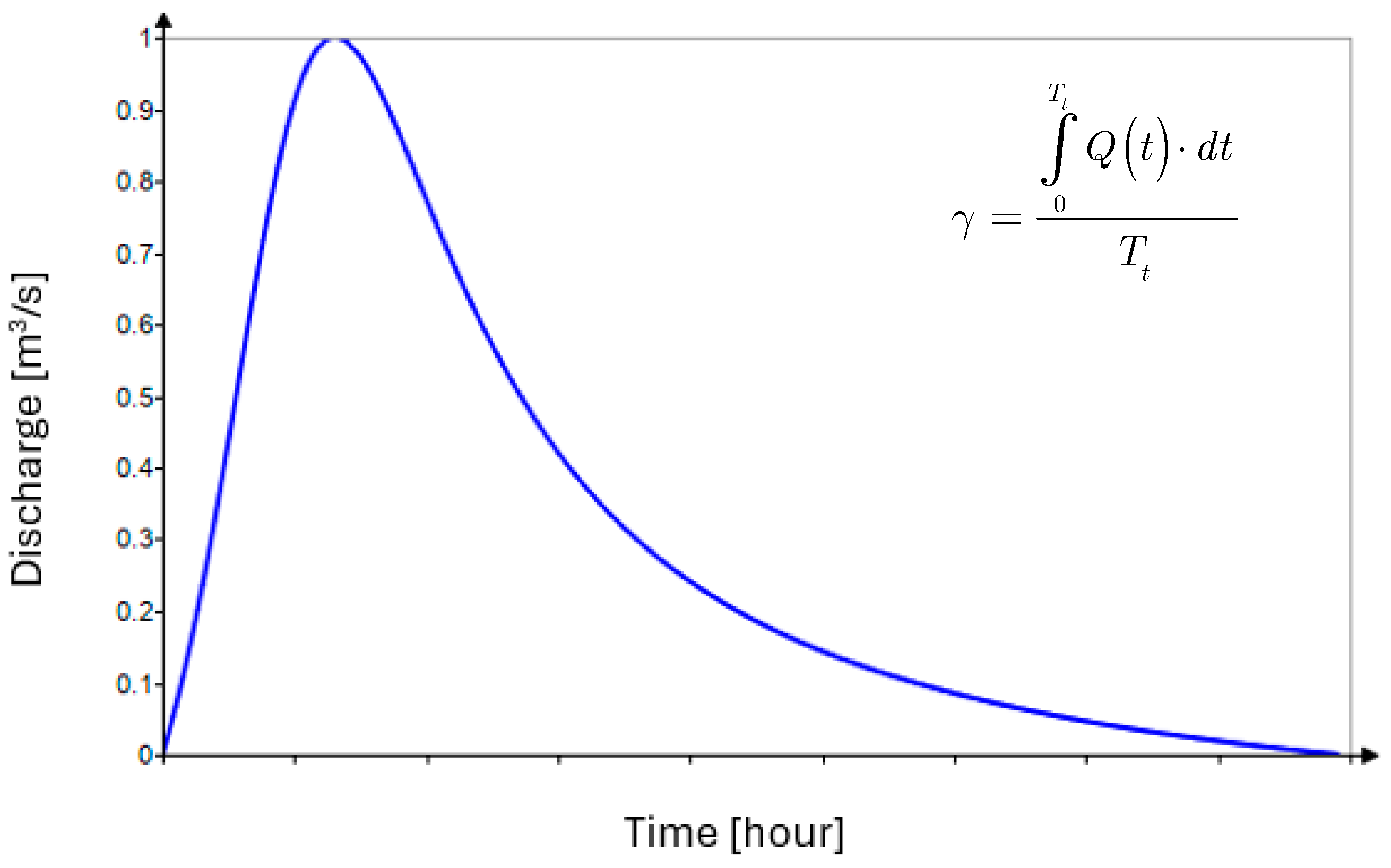
The analytical function models theoretical floods for a shape coefficient between $0.15\le \gamma \le 0.50$ and $2\le {\displaystyle \frac{T}{T_c}}\le 6.5$. The graphical representation of the shape coefficient is shown in Figure 1.

Appendix B presents a line of VBA code for automatically determining and plotting the Cadariu flood wave in Excel.

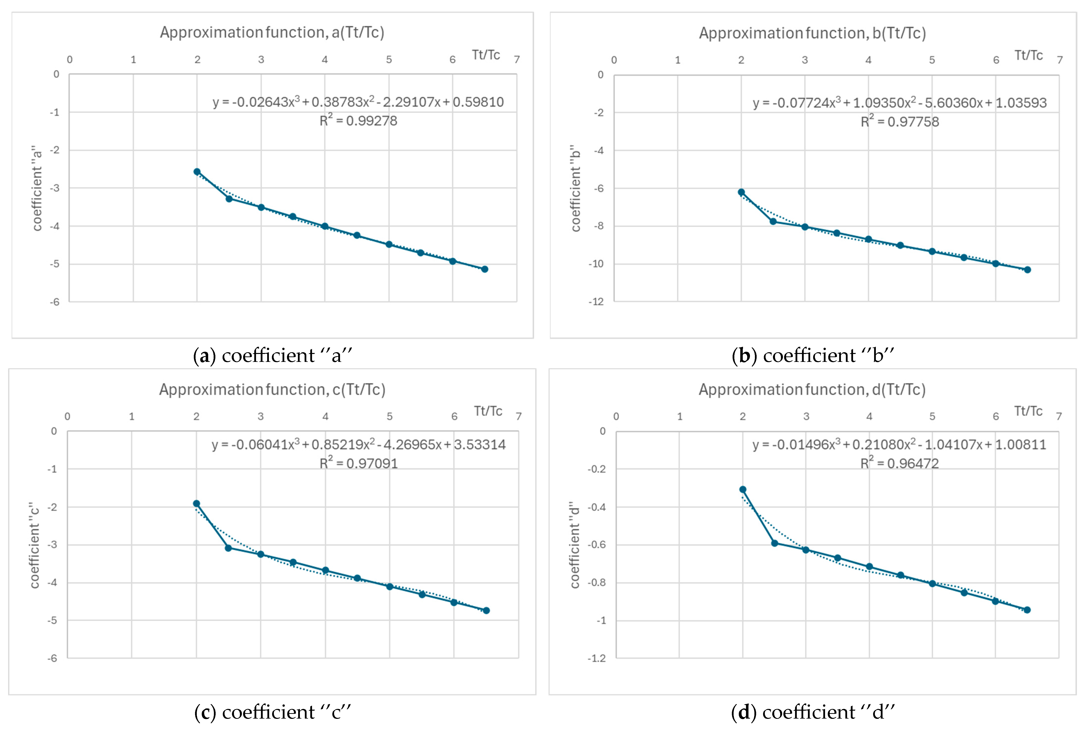
Considering that the determination of parameter $A$ requires solving a nonlinear equation, an attempt was made to find approximate relations for its estimation and to facilitate the use of Cadariu’s relation by eliminating this difficulty. Thus, taking into account that parameter $A$ is obtained by solving the nonlinear Equation (9), as a function of the ratio $2\le {\displaystyle \frac{T}{T_c}}\le 6.5$, as well as the flood shape parameter $0.15\le \gamma \le 0.50$, a relation was developed for estimating $A$. The relation has an exponential form with a logarithmic argument (for more information see Appendix A).

The approximation function is:

$$A\left(\gamma \right)=\exp \left(a+b\cdot \ln \left(\gamma \right)+c\cdot \ln {\left(\gamma \right)}^2+d\cdot \ln {\left(\gamma \right)}^3\right).$$

(11)

Table 1. The coefficients of Equation (11) for Cadariu’s function.

$\mathbf{The}\mathbf{Values}\mathbf{of}\mathbf{the}\mathbf{Coefficients}\mathbf{of}\mathbf{the}\mathbf{Approximation}\mathbf{Relation},0.15\le \mathit{\gamma }\le 0.50$
$\frac{\mathit{T}}{{\mathit{T}}_{\mathit{c}}}$	a	b	c	d
2	−2.55835787	−6.184919402	−1.90284695	−0.306908269
2.5	−3.275893791	−7.760612647	−3.078643546	−0.589138834
3	−3.498941124	−8.033858395	−3.250431222	−0.625262443
3.5	−3.749102464	−8.351235857	−3.452406079	−0.668014285
4	−4.002425016	−8.685534635	−3.668117509	−0.714053759
4.5	−4.002425	−9.012087248	−3.879172318	−0.758946884
5	−4.245302	−9.343317759	−4.096078957	−0.805498724
5.5	−4.481729	−9.669394123	−4.310917569	−0.851717451
6	−4.708091	−9.987460462	−4.521511374	−0.897107836
6.5	−4.923748	−10.29905649	−4.728537305	−0.94176487

presents the coefficients of the approximation function over the definition domain of the flood shape coefficient, $\gamma$.

Furthermore, approximation relations for each coefficient in relation (11) were developed based on the values in Table 1, depending on the ratio ${\displaystyle \frac{T}{T_c}}$, so that finally an approximation relation (a two-dimensional relation) can be written:

$$A\left({\displaystyle \frac{T}{T_c}},\gamma \right)=\exp \left(a^{\ast }+b^{\ast }\cdot \ln \left(\gamma \right)+c^{\ast }\cdot \ln {\left(\gamma \right)}^2+d^{\ast }\cdot \ln {\left(\gamma \right)}^3\right).$$

(12)

The coefficients of relation (12) have the approximate expressions according to

Table 2. The coefficients of Equation (12) for Cadariu’s function.

$a^{\ast }=-0.02643\cdot {\left({\displaystyle \frac{T_t}{T_c}}\right)}^3+0.38783\cdot {\left({\displaystyle \frac{T_t}{T_c}}\right)}^2-2.29107\cdot {\displaystyle \frac{T_t}{T_c}}+0.59810$	(13)
$b^{\ast }=-0.07724\cdot {\left({\displaystyle \frac{T_t}{T_c}}\right)}^3+1.09350\cdot {\left({\displaystyle \frac{T_t}{T_c}}\right)}^2-5.60360\cdot {\displaystyle \frac{T_t}{T_c}}+1.03593$	(14)
$c^{\ast }=-0.06041\cdot {\left({\displaystyle \frac{T_t}{T_c}}\right)}^3+0.85219\cdot {\left({\displaystyle \frac{T_t}{T_c}}\right)}^2-4.26965\cdot {\displaystyle \frac{T_t}{T_c}}+3.53314$	(15)
$d^{\ast }=-0.01496\cdot {\left({\displaystyle \frac{T_t}{T_c}}\right)}^3+0.21080\cdot {\left({\displaystyle \frac{T_t}{T_c}}\right)}^2-1.04107\cdot {\displaystyle \frac{T_t}{T_c}}+1.00811$	(16)

.

Thus, with parameter $A$ determined (a function of $0.15\le \gamma \le 0.50$ and $2\le {\displaystyle \frac{T}{T_c}}\le 6.5$), parameters $B$ and $C$ are determined with relations (6) and (7).

2.2. Triangular Function

The triangular relationship in synthetic flood estimation is a simplified but very useful concept in hydrology, used especially in areas with limited or non-existent hydrometric data. This relationship involves approximating the hydrograph of a flood by a triangular hydrograph, that is, an idealized geometric shape, defined by three key points: the beginning, the peak, and the end of the flood.

It is a semi-empirical method of constructing the flood hydrograph based on some basin hydrological parameters, assuming that the shape of the hydrograph can be represented as an isosceles or asymmetric triangle.

Although it has some advantages, this approach ignores the real variations of intensity—it does not capture the real shape of the flood well and may underestimate/overestimate secondary peaks or slow decreases.

The wave relation has the following expressions [21,22,23]:

If $0<t\le T_c$:

$$Q\left(t\right)=Q_{p\%}\cdot {\displaystyle \frac{t}{T_c}}.$$

(17)

If $T_c<t\le T_t$:

$$Q\left(t\right)=Q_{p\%}-Q_{p\%}\cdot {\displaystyle \frac{t-T_c}{T_t-T_c}}.$$

(18)

2.3. Weibull Probability Function

The 3-parameter Weibull distribution is a flexible distribution increasingly used in the statistical analysis of maximum annual discharges, including in the context of synthetic flood estimation. Due to its ability to model different shapes of the frequency curve (symmetric, asymmetric, long-tailed, or short-tailed), it is a valuable alternative to the classical distributions (Pearson III).

The probability density function PDF of the Weibull distribution is:

$$Q\left(t\right)={\displaystyle \frac{\alpha }{\beta }}\cdot {\left({\displaystyle \frac{t-\delta }{\beta }}\right)}^{\alpha -1}\cdot \exp \left(-{\left({\displaystyle \frac{t-\delta }{\beta }}\right)}^{\alpha }\right),$$

(19)

where $\alpha ,\beta ,\delta$ are the shape, scale, and position parameters. By scaling the density function with the flow associated with the desired probability ($Q_{p\%}$), the hydrograph associated with the desired probability is drawn.

The equations necessary to estimate the distribution parameters and represent the unit hydrograph are the following:

$$\left({\alpha }^2-\alpha \right)\cdot {\left({\displaystyle \frac{T_c-\delta }{\beta }}\right)}^{\alpha -2}={\alpha }^2\cdot {\left({\displaystyle \frac{T_c-\delta }{\beta }}\right)}^{2\cdot \alpha -2},$$

(20)

$${\displaystyle \frac{\alpha }{\beta }}\cdot \exp \left(-{\left({\displaystyle \frac{T_c-\delta }{\beta }}\right)}^{\alpha }\right)\cdot {\left({\displaystyle \frac{T_c-\delta }{\beta }}\right)}^{\alpha -1}=1,$$

(21)

$${\displaystyle \frac{{\displaystyle \underset{0}{\overset{T_t}{\int }}\frac{\alpha }{\beta }\cdot {\left(\frac{t-\delta }{\beta }\right)}^{\alpha -1}\cdot \exp \left(-{\left(\frac{t-\delta }{\beta }\right)}^{\alpha }\right)\cdot dt}}{T_t}}=\gamma .$$

(22)

2.4. Bazin’s Relationship

Bazin’s relation has the following expression [23,24]:

$$Q\left(t\right)={\left({\displaystyle \frac{t}{T_c}}\right)}^{\alpha }\cdot \exp \left(a\left(1-{\displaystyle \frac{t}{T_c}}\right)\right),$$

(23)

where $a$ is a shape parameter. By scaling the density function with the flow rate corresponding to the desired probability ($Q_{p\%}$), the hydrograph corresponding to the desired probability is drawn.

The equations necessary to estimate the parameter $a$ and to construct the unitary hydrograph are the following:

$${\left({\displaystyle \frac{T_c}{T_c}}\right)}^{\alpha }\cdot \exp \left(a\left(1-{\displaystyle \frac{T_c}{T_c}}\right)\right)=1,$$

(24)

$${\displaystyle \frac{{\displaystyle \underset{0}{\overset{T_t}{\int }}{\left(\frac{t}{T_c}\right)}^{\alpha }\cdot \exp \left(a\left(1-\frac{t}{T_c}\right)\right)\cdot dt}}{T_t}}=\gamma .$$

(25)

By solving these two relations simultaneously, the value of the hydrograph shape parameter is determined. Usually, $a\in [2,5]$.

As in the case of the Cadariu function, approximation relations for the parameter $a$ have been developed. The general equations are identical to those of the Cadariu function, namely, Equations (11) and (12).

The parameters of the two functions are found according to

Table 3. The coefficients of Equation (11) for Bazin’s function.

$\mathbf{The}\mathbf{Values}\mathbf{of}\mathbf{the}\mathbf{Coefficients}\mathbf{of}\mathbf{the}\mathbf{Approximation}\mathbf{Relation},0.15\le \mathit{\gamma }\le 0.50$
$\frac{\mathit{T}}{{\mathit{T}}_{\mathit{c}}}$	a	b	c	d	e	f
2	−1.12794221	−7.07974994	−6.44171618	−4.05625883	−1.27172799	−0.15897765
2.5	−1.13894691	−6.0007075	−5.40106964	−3.58599312	−1.17870543	−0.15384214
3	−1.32029933	−5.54586396	−4.9279017	−3.33657136	−1.11342629	−0.14715703
3.5	−1.54409267	−5.38040767	−4.78102184	−3.26545299	−1.095289	−0.1452574
4	−1.76878258	−5.34500847	−4.78522042	−3.27890647	−1.10008833	−0.14576199
4.5	−1.98040274	−5.36654005	−4.85167046	−3.32368167	−1.11204981	−0.14682241
5	−2.17436975	−5.40844047	−4.93410042	−3.37108371	−1.12241815	−0.14738493
5.5	−2.34921213	−5.44939491	−5.00460659	−3.40335892	−1.12565382	−0.14676805
6	−2.50580133	−5.48040858	−5.0521281	−3.41417596	−1.1200563	−0.14480169
6.5	−2.64523243	−5.4960274	−5.07025297	−3.40022513	−1.10490038	−0.14144129

and

Table 4. The coefficients of Equation (12) for Bazin’s function.

$a^{\ast }=0.00328426\cdot {\left({\displaystyle \frac{T_t}{T_c}}\right)}^5-0.07909525\cdot {\left({\displaystyle \frac{T_t}{T_c}}\right)}^4+0.75116726\cdot {\left({\displaystyle \frac{T_t}{T_c}}\right)}^3-3.48055199\cdot {\left({\displaystyle \frac{T_t}{T_c}}\right)}^2+7.39025555\cdot {\displaystyle \frac{T_t}{T_c}}-6.83392778$	(26)
$b^{\ast }=0.00770080\cdot {\left({\displaystyle \frac{T_t}{T_c}}\right)}^5-0.19169427\cdot {\left({\displaystyle \frac{T_t}{T_c}}\right)}^4+1.90666378\cdot {\left({\displaystyle \frac{T_t}{T_c}}\right)}^3-9.48787642\cdot {\left({\displaystyle \frac{T_t}{T_c}}\right)}^2+23.58764833\cdot {\displaystyle \frac{T_t}{T_c}}-28.73407776$	(27)
$c^{\ast }=0.00485878\cdot {\left({\displaystyle \frac{T_t}{T_c}}\right)}^5-0.12889448\cdot {\left({\displaystyle \frac{T_t}{T_c}}\right)}^4+1.37691567\cdot {\left({\displaystyle \frac{T_t}{T_c}}\right)}^3-7.37234102\cdot {\left({\displaystyle \frac{T_t}{T_c}}\right)}^2+19.56567862\cdot {\displaystyle \frac{T_t}{T_c}}-25.19207655$	(28)
$d^{\ast }=0.00013697\cdot {\left({\displaystyle \frac{T_t}{T_c}}\right)}^5-0.01314449\cdot {\left({\displaystyle \frac{T_t}{T_c}}\right)}^4+0.24646854\cdot {\left({\displaystyle \frac{T_t}{T_c}}\right)}^3-1.85668399\cdot {\left({\displaystyle \frac{T_t}{T_c}}\right)}^2+6.13971788\cdot {\displaystyle \frac{T_t}{T_c}}-10.67619169$	(29)
$e^{\ast }=-0.00083093\cdot {\left({\displaystyle \frac{T_t}{T_c}}\right)}^5+0.01622651\cdot {\left({\displaystyle \frac{T_t}{T_c}}\right)}^4-0.10858978\cdot {\left({\displaystyle \frac{T_t}{T_c}}\right)}^3+0.25425650\cdot {\left({\displaystyle \frac{T_t}{T_c}}\right)}^2+0.06744222\cdot {\displaystyle \frac{T_t}{T_c}}-1.78884082$	(30)
$f^{\ast }=-0.00020810\cdot {\left({\displaystyle \frac{T_t}{T_c}}\right)}^5+0.00445688\cdot {\left({\displaystyle \frac{T_t}{T_c}}\right)}^4-0.03578577\cdot {\left({\displaystyle \frac{T_t}{T_c}}\right)}^3+0.13195328\cdot {\left({\displaystyle \frac{T_t}{T_c}}\right)}^2-0.21440557\cdot {\displaystyle \frac{T_t}{T_c}}-0.03650750$	(31)

.

2.5. Vladimirescu’s Relationship

Vladimirescu’s relation is defined by the two branches (increasing and decreasing) and has the following expressions [21,25,26]:

If $0<t\le T_c$:

$$Q\left(t\right)={\left({\displaystyle \frac{t}{T_c}}\right)}^n.$$

(32)

If $T_c<t\le T_t$:

$$Q\left(t\right)=\exp \left(-\beta \cdot \left(t-T_c\right)\right),$$

(33)

where the parameter values $n,\beta$ are determined regionally based on historical data. They usually vary between $n\in [1.5,3]$ and $\beta \in [0.05,0.3]$.

3. Real Case Data

The performances of the analyzed distributions are verified on case studies, in which the values of the characteristic parameters of the flood waves are determined regionally, for locations with different statistical, hydrological, and morphometric characteristics.

The regionally determined parameters are presented in

Table 5. Regionally determined parameter values (provided).

Case Study	Watershed $\mathit{A}$	Max. Flow ${\mathit{Q}}_{1\%}$	Total Time ${\mathit{T}}_{\mathit{t}}$	Time to Peak ${\mathit{T}}_{\mathit{p}}$	Shape Coefficient γ
	(km2)	(m3/s)	(hR)	(hR)	(-)
1	28.0	112	40	8	0.25
2	61.0	148	60	12	0.26
3	102	170	35	7	0.35
4	135	118	89	13	0.3
5	189	200	50	9	0.35
6	270	265	62	11	0.35
7	1165	360	120	30	0.30
8	1959	438	140	35	0.31

.

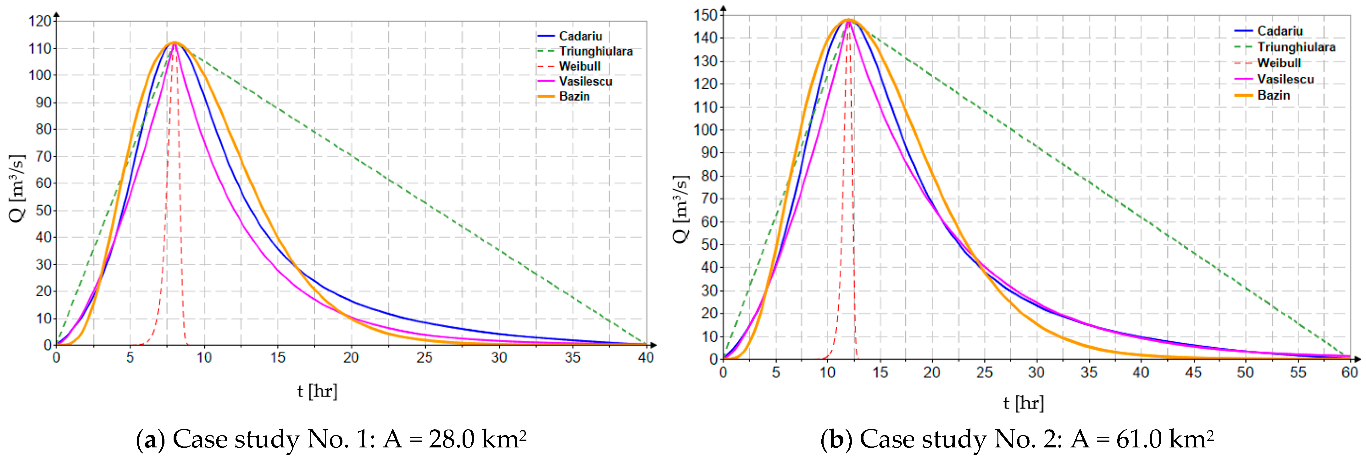
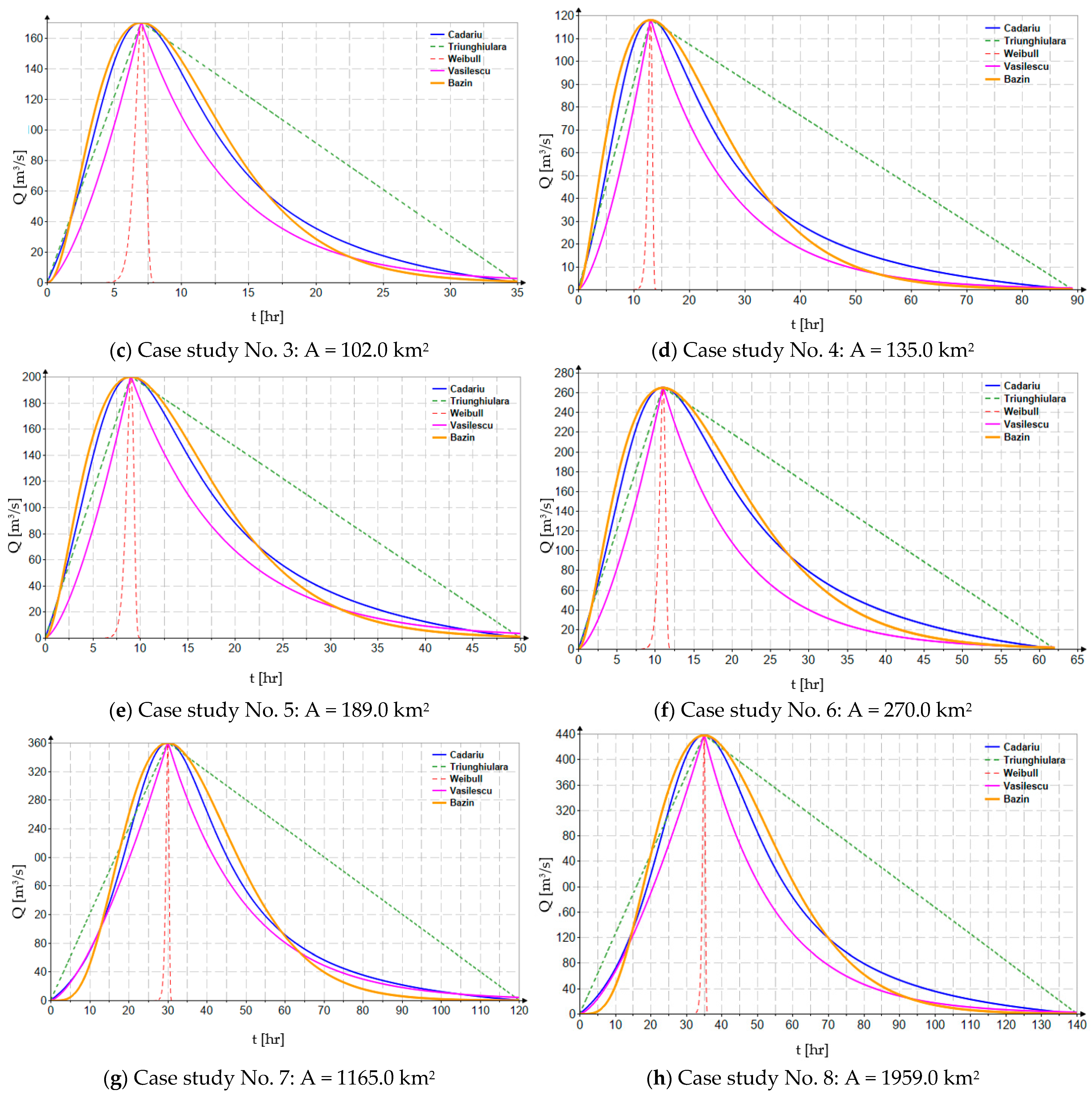
Figure 2 presents the results obtained for representative case studies in terms of the characteristics and particularities of the river basins.

In the analysis conducted on synthetic hydrograph modeling using probability density functions, the focus was placed on their ability to accurately reproduce the main hydrological characteristics of flood waves: peak discharge, rise time, total flood duration, and shape coefficient. These four conditions are fundamental requirements for constructing a realistic synthetic hydrograph, particularly in ungauged catchments where measured data are lacking.

Among the tested functions, the rational function proposed by Cadariu consistently demonstrated superior adaptability to these conditions. This function, defined by a ratio of polynomials and calibrated according to the basin’s characteristic parameters, provides high formal flexibility, allowing for simultaneous and controlled representation of both the rise time and the shape of the recession limb. Compared to other commonly used functions (e.g., Pearson type III, gamma, beta, log-normal, etc.), the Cadariu function allows more direct control over the hydrograph asymmetry and the positioning of the peak discharge.

Another important aspect is the precise compliance with the total flood duration, without the need for artificial truncation of the density function. While other PDFs require empirical adjustments or numerical methods to close the curve at a given duration, the rational function strictly accommodates this limit simply through the choice of functional parameters, thus facilitating its integration into computational simulation algorithms.

Regarding the flood shape coefficient (often defined as the ratio between rise time and total duration), the Cadariu function is one of the few that allows direct control over this ratio while maintaining mathematical continuity and full differentiability—essential characteristics for propagation analyses and hydraulic modeling.

It is also worth mentioning Bazin’s empirical relationship, which, although formally simpler, produces similar results in terms of the general shape of the hydrograph. It relies on a single shape parameter, and its mathematical expressions are significantly simpler, making it attractive for practical applications or rapid assessment methods. Thus, in contexts where simplicity and computational speed are priorities, the use of Bazin’s relationship may be justified and efficient, with the note that the accuracy of the results still depends on the correct selection of the characteristic parameter.

Table 6. Resulting flood wave volumes.

Case Study	Flood Wave Volumes (hm3 = 1,000,000 m3)
	Real	Cadariu	Triangular	Weibull	Vasilescu	Bazin
	(hm3)	(hm3)	(hm3)	(hm3)	(hm3)	(hm3)
1	4	4	8.1	0.4	3.3	4
2	8.3	8.3	16	0.5	7.8	8.3
3	7.5	7.5	10.7	0.6	5.7	7.5
4	11.3	11.3	18.9	0.4	8.2	11.3
5	12.6	12.6	18	0.7	9.7	12.6
6	20.7	20.7	29.6	1	13.7	20.7
7	46.7	46.7	77.8	1.3	41.2	46.7
8	68.4	68.4	110.4	1.6	53.4	68.4

presents the volumes (in hm³) of the synthetic flood waves obtained using the analyzed probability functions.

The errors between the resulting estimated volume values and the actual ones are highlighted in

Table 7. Relative errors of flood volumes.

Case Study	Relative Mean Errors, (%)
	Cadariu	Triangular	Weibull	Vasilescu	Bazin
1	0	−103	90	18	0
2	0	−93	94	6	0
3	0	−43	92	24	0
4	0	−67	96	27	0
5	0	−43	94	23	0
6	0	−43	95	34	0
7	0	−67	97	12	0
8	0	−61	98	22	0

. These errors were determined based on the RME (relative mean error) criteria.

It can be seen that there are large percentage differences between the synthetic flood volumes.

Cadariu’s function and Bazin’s method show zero relative errors (0%), meaning they are explicitly calibrated to conserve the flood volume. They respect a fundamental condition: the total volume of the synthetic hydrograph must equal the observed one or that imposed by hydrological assumptions.

The triangular function has very large and negative deviations (up to −103%), indicating that this simple geometric approach consistently underestimates the flood volume. The main reason is that the triangular function, although it can roughly reproduce the rise and recession times, cannot correctly capture the asymmetry and temporal extension of real floods.

The Weibull function shows large positive errors (90–98%), i.e., it almost doubles the real volume. This is due to its parametric form, where calibration based on characteristic times leads to an exaggerated extension of the flood recession limb, adding a significant artificial volume.

The Vasilescu function shows more moderate errors (6–34%), but still consistent. This suggests that the method captures the asymmetry of the flood better, but it is not strictly calibrated for volume conservation.

The flood volume is a crucial parameter in applied hydrology, as it determines the dimensioning of hydraulic structures: reservoirs, dams, levees, or mitigation basins must be designed not only for the maximum flow (Q_max) but also for the total volume to be diverted or stored. It also controls the efficiency of flood protection measures, where a high maximum flow, but of short duration, has very different impacts compared to a lower flow with a high volume (prolonged flooding, infiltration, and dam saturation). In downstream propagation studies, the volume controls the shape of the hydrograph. An error of 90–100% in the flood volume leads to completely misleading predictions of downstream water levels.

Volume conservation is a fundamental requirement, where any synthetic function must respect the balance between precipitation, losses, and effective runoff. The parameters must be calibrated simultaneously on several criteria: not only on the rise and fall times but also on the volume and asymmetry. Without such calibration, the results can be misleading—a function that correctly reproduces Q_max but has twice the actual volume is not valid for engineering purposes.

Parametric functions (Weibull and Vasilescu) can be useful but require parameter adjustment by optimization methods (e.g., minimizing the squared error between the observed and synthetic hydrographs) to avoid systematic volume errors.

4. Conclusions

The comparative analysis of density functions applicable in the modeling of synthetic hydrographs highlighted the clear and consistent advantages of the rational Cadariu function in satisfying the essential hydrological requirements: maximum discharge, rise time, total flood duration, and shape coefficient.

Due to its parametric flexibility, precise adjustment capacity, and mathematical coherence, the Cadariu function ensures a faithful rendering of real flood shapes, without empirical adjustments or artificial duration limitations. It proves to be a robust and rigorous tool, especially for analytical applications and detailed simulations in undeveloped basins.

On the other hand, the Bazin relation remains a viable and efficient alternative in contexts where computational resources are limited, and simplicity of implementation is essential. Even though it uses a single shape parameter, it manages to render the main characteristics of the hydrograph well enough, offering a reasonable compromise between complexity and accuracy.

In conclusion, the choice of modeling function must take into account the purpose of the analysis, the desired level of detail, and the availability of data, but for high-fidelity applications, the Cadariu rational function remains the preferable option, while the Bazin relation is advisable for rapid and operational assessments.

References

1. Bejenaru, G.; Castravet, T.; Dilan, V. Hydrological Calculations; Print Caro Publishing House: Chisinau, Moldova, 2020. [Google Scholar]
2. Banach, W. Determination of synthetic flood hydrograph in ungauged catchments. Infrastrukt. I Ekol. Teren. Wiej. 2011, 12, 147–156. [Google Scholar]
3. Petroselli, A.; Piscopia, R.; Grimaldi, S. Design discharge estimation in small and ungauged basins: EBA4SUB framework sensitivity analysis. J. Agric. Eng. 2020, 51, 107–118. [Google Scholar] [CrossRef]
4. Yue, S.; Taha, B.M.J.; Bobee, B.; Legendre, P.; Bruneau, P. Approach for describing statistical properties of flood hydrograph. J. Hydrol. Eng. 2002, 7, 147–153. [Google Scholar] [CrossRef]
5. Haktanir, T.; Sezen, N. Suitability of two-parameter gamma distribution and three-parameter beta distribution as synthetic hydrographs in anatolia. Hydrol. Sci. J. 1990, 35, 167–184. [Google Scholar] [CrossRef]
6. Bhunya, P.K.; Mishra, S.K.; Berndtsson, R. Simplified two parameter gamma distribution for derivation of synthetic unit hydrograph. J. Hydrol. Eng. 2003, 8, 226–230. [Google Scholar] [CrossRef]
7. Bhunya, P.K.; Berndtsson, R.; Ojha, C.S.P.; Mishra, S.K. Suitability of gamma, chi-square, weibull and beta distributins as synthetic unit hydrographs. J. Hydrol. 2007, 334, 28–38. [Google Scholar] [CrossRef]
8. Bhattacharjya, R.K. Optimal design of unit hydrographs using probability distribution and genetic algorithms. Sadhana 2004, 29, 499–508. [Google Scholar] [CrossRef]
9. Bhunya, P.K.; Mishra, S.K.; Ojha, C.S.P.; Berndtsson, R. Parameter estimation of beta-distribution for unit hydrograph derivation. J. Hydrol. Eng. 2004, 9, 325–332. [Google Scholar] [CrossRef]
10. Bhunya, P.K.; Singh, P.K.; Mishra, S.K. Fréchet and chi-square parametric expressions combined with horton ratios to derive a synthetic unit hydrograph. Hydrol. Sci. 2009, 54, 274–286. [Google Scholar] [CrossRef]
11. Nadarajah, S. Probability models for unit hydrograph derivation. J. Hydrol. 2007, 344, 185–189. [Google Scholar] [CrossRef]
12. Kleiber, C. A guide to the Dagum distributions. In Modeling Income Distributions and Lorenz Curves; Springer: New York, NY, USA, 2008; pp. 97–117. [Google Scholar] [CrossRef]
13. Ashkar, F.; Mahdi, S. Fitting the log-logistic distribution by generalized moments. J. Hydrol. 2006, 328, 694–703. [Google Scholar] [CrossRef]
14. Ghorbani, M.A.; Kashani, M.; Zeynali, S. Development of synthetic unit hydrograph using probability models. Res. Civ. Environ. Eng. 2013, 1, 54–66. [Google Scholar]
15. Anghel, C.G. Revisiting the Use of the Gumbel Distribution: A Comprehensive Statistical Analysis Regarding Modeling Extremes and Rare Events. Mathematics 2024, 12, 2466. [Google Scholar] [CrossRef]
16. Anghel, C.G.; Stanca, S.C.; Ilinca, C. Two-Parameter Probability Distributions: Methods, Techniques and Comparative Analysis. Water 2023, 15, 3435. [Google Scholar] [CrossRef]
17. Anghel, C.-G.; Ianculescu, D. An In-Depth Statistical Analysis of the Pearson Type III Distribution Behavior in Modeling Extreme and Rare Events. Water 2025, 17, 1539. [Google Scholar] [CrossRef]
18. Anghel, C.G.; Ianculescu, D. Probabilistic Forecasting of Peak Discharges Using L-Moments and Multi-Parameter Statistical Models. Water 2025, 17, 1908. [Google Scholar] [CrossRef]
19. Anghel, C.G.; Ianculescu, D. Application of the GEV Distribution in Flood Frequency Analysis in Romania: An In-Depth Analysis. Climate 2025, 13, 152. [Google Scholar] [CrossRef]
20. Cadariu, R. Dimensionless analytical model for the shape of singular theoretical floods. Hidrotehnica 1979, 24, 124–125. [Google Scholar]
21. Diacon, C.; Serban, P. Hydrological Syntheses and Regionalizations; Technical Publishing House: Bucharest, Romania, 1994. [Google Scholar]
22. Constantinescu, M.; Golstein, M.; Haram, V.; Solomon, S. Hydrology; Technical Publishing House: Bucharest, Romania, 1956. [Google Scholar]
23. Pieyns, J. Cours D’hydrologie; Centre de Formation de Techniciens Hydrologues, ORSTOM, avril: Niamey, Romania, 1978. [Google Scholar]
24. Laborde, J.-P. Éléments D’hydrologie de Surface; École Polytechnique de l’Université de Nice–Sophia Antipolis, Département Hydroinformatique et Ingénierie de l’Eau: Biot, France, 2009. [Google Scholar]
25. Vladimirescu, I. Basics of Technical Hydrology; Technical Publishing House: Bucharest, Romania, 1984. [Google Scholar]
26. Stănescu, V.A. Hydrological Studies. Volume XXXIV: Mathematical Models for Determining Critical Flood Waves; Institute of Meteorology and Hydrology: Bucharest, Romania, 1972. [Google Scholar]
Figure 1. Representation of the flood shape coefficient.
Stats 08 00100 g001
Figure 2. Resulting synthetic flood waves.
Stats 08 00100 g002aStats 08 00100 g002b