Model-Free Feature Screening Based on Data Aggregation for Ultra-High-Dimensional Longitudinal Data

Abstract

Ultra-high dimensional longitudinal data feature screening procedures are widely studied, but most require model assumptions. The screening performance of these methods may not be excellent if we specify an incorrect model. To resolve the above problem, a new model-free method is introduced where feature screening is performed by sample splitting and data aggregation. Distance correlation is used to measure the association at each time point separately, while longitudinal correlation is modeled by a specific cumulative distribution function to achieve efficiency. In addition, we extend this new method to handle situations where the predictors are correlated. Both methods possess excellent asymptotic properties and are capable of handling longitudinal data with unequal numbers of repeated measurements and unequal intervals between repeated measurement time points. Compared to other model-free methods, the two new methods are relatively insensitive to within-subject correlation, and they can help reduce the computational burden when applied to longitudinal data. Finally, we use some simulated and empirical examples to show that both new methods have better screening performance.

1. Introduction

Longitudinal data, characterized by repeated measurements of the same subjects over some time, are common in many scientific fields, including public health, psychology, and sociology. Traditional methods, such as linear mixed models (LMMs), are widely used to analyze longitudinal supervised problems. However, as the number of predictors, p, grows, these methods are limited by “the curse of dimensionality”. Even if these problems have a seemingly large sample size, n, it may actually be far smaller than p. This is more commonly called the ultra-high-dimensional setting, defined by Fan and Lv [1] as $logp=O\left(n^{\alpha }\right)$ for some $\alpha \in (0,1/2)$. On the other hand, technological developments have made it possible to obtain high-throughput data through repeated measurements of subjects. Therefore, it is essential to develop some new methods capable of handling the above data.

Since only a few predictors are associated with the response in the ultra-high-dimensional setting (i.e., sparsity), feature screening is a common method to deal with these problems. For early work on ultra-high-dimensional longitudinal data, sure independence screening for varying-coefficient models was firstly proposed [2], while subsequent studies developed further, including partially linear models [3], additive models [4], and rank regression models [5]. However, these methods rely on parametric or semi-parametric models, which may be insufficient for accurate model specification in the big data era. To address this, we agree with Zhu et al. [6] that model-free methods are more appealing, as they rely only on a general model framework.

Currently, research on model-free methods for cross-sectional data has made great progress. The primary approach of these methods is to measure the marginal dependence, such as distance correlation (DC) [7], martingale difference correlation [8], conditional distance correlation (CDC) [9], and covariate information number [10]. Recently, some studies have also applied these methods to survival data and other types of data by improving the methods originally designed for cross-sectional data [11,12,13]. However, up to now, studies applying model-free feature screening procedures to longitudinal data are still rare, with the main challenge being that repeated measurements between subjects are correlated.

Since Székely et al. [14] proposed DC and Wang et al. [15] proposed CDC, the two methods have been widely applied in feature screening, e.g., the studies by Li et al. [7] and Chen [16] are based on DC, while the studies by Wen et al. [9] and Lu and Lin [17] are based on CDC. Consequently, the aim of this study is to improve DC and CDC for better performance in longitudinal data. Recently, the sample splitting and data aggregation methods are frequently used in feature screening, such as Zhong et al. [12] and Dai et al. [18]. These studies provide us with an idea of handling ultra-high-dimensional longitudinal data.

We first introduce a new method called longitudinal distance correlation sure independence screening (LDCS) in this study. The new method uses DC to measure marginal dependence at each time point separately and then aggregates the results using a cumulative distribution function (CDF) used in Zhong et al. [12]. We also make a simple extension of LDCS to handle situations where predictors are correlated. The method is based on CDC, so we call it longitudinal conditional distance correlation sure independence screening (LCDCS). The two new methods have some distinct advantages. For example, compared to existing longitudinal data feature screening procedures, the two methods are model-free, which enables them to perform better in some complex situations. Additionally, compared to existing model-free feature screening procedures, LDCS and LCDCS use the sample-splitting and data aggregation methods, making them relatively insensitive to within-subject correlation. Moreover, the computational burden is lower than that of methods that directly apply dependence measures to longitudinal data.

In Section 2, we propose our methods and provide their asymptotic properties. Section 3 presents several simulated and empirical examples to compare the performance of our methods with that of some other feature screening procedures. Section 4 provides a brief discussion of the article. Appendix A contains the technical proofs of all theorems, and Appendix B presents a simple sensitivity analysis.

2. Materials and Methods

2.1. Model Setup

We consider the following longitudinal data, $\{({\mathbf{y}}_{im},{\mathbf{X}}_{im},{\mathbf{Z}}_{im}),1\le i\le n,1\le m\le M_i\}$ denotes the measurement at the mth measurement time point $t_m$ for the ith subject, where ${\mathbf{y}}_{im}\in R^q$ is the response vector correlated with the predictor vector ${\mathbf{X}}_{im}\in R^p$ and the conditional predictor vector ${\mathbf{Z}}_{im}\in R^r$. Here, n represents the number of subjects, and $M_i$ denotes the repeated measurements for the ith subject. We allow the measurement intervals at different time points to be unequal and repeated measurements for each subject to vary. Furthermore, we define the total measurements as $N={\sum }_{i=1}^n{M}_i$ and the maximum of $M_i$ as M.

2.2. Marginal Screening Procedure

We assume that n is much less than p, and only a few predictors are associated with $\mathbf{y}$. Let $F(\mathbf{y}|\mathbf{X})$ denote the conditional distribution function of $\mathbf{y}$, given $\mathbf{X}$. The index set of important predictors can be defined as

$$D=\{k:F(\mathbf{y}|\mathbf{X})\mathrm{functionally}\mathrm{depends}\mathrm{on}{X}_k,k=1,\dots ,p\},$$

without assuming a specific regression model. We define the number of important predictors as $L_0=\left|D\right|$, the cardinality of D, and denote $D^c$ as the index set of unimportant predictors. Similar to most screening procedures, our screening goal is to estimate D conservatively so that all important predictors can be retained.

DC was proposed to quantify the association between two random vectors [14]. For details, they defined DC between $\mathbf{y}$ and $\mathbf{X}$ as the square root of

$$dCo{r}^2(\mathbf{X},\mathbf{y})={\displaystyle \frac{dCo{v}^2(\mathbf{X},\mathbf{y})}{\sqrt{dCo{v}^2(\mathbf{X},\mathbf{X})dCo{v}^2(\mathbf{y},\mathbf{y})}}},$$

where distance covariance is defined as the square root of

$$dCo{v}^2(\mathbf{X},\mathbf{y})={\int }_{R^{p+q}}{\parallel {\varphi }_{\mathbf{X},\mathbf{y}}(\mathbf{s},\mathbf{t})-{\varphi }_{\mathbf{X}}(\mathbf{s}){\varphi }_{\mathbf{y}}(\mathbf{t})\parallel }^{2}p(\mathbf{s},\mathbf{t})d\mathbf{s}d\mathbf{t},$$

where $p(\mathbf{s},\mathbf{t})$ is a known function, and $\varphi (·)$ denotes the characteristic function.

DC is an excellent dependence measure capable of detecting the relationship between predictors and response for cross-sectional data. However, the screening performance of DC in longitudinal data is not as satisfactory, as can be seen in the simulation study. In this article, we consider a sample splitting and data aggregation method used by Zhong et al. [12] to improve the application of DC in longitudinal data feature screening.

First, we assume that $t_1<t_2<\dots <t_M$. We split the longitudinal data into M parts based on the difference of $t_m$, and we denote DC between $X_{km}(k=1,\dots ,p)$ and ${\mathbf{y}}_m$ at the mth time point $t_m$ by $D{C}_k\left(t_m\right)=dCo{r}^2(X_{km},{\mathbf{y}}_m)$. We construct the following aggregated statistic:

$${\omega }_k={\int }_{u\in R}D{C}_k\left(u\right)dF\left(u\right),$$

where $F\left(u\right)$ is a specific CDF. For instance, taking $F(·)$ as the CDF of the true time variable T, and then the aggregated statistic becomes

$${\omega }_k={\int }_{t\in R}D{C}_k\left(t\right)dF\left(t\right)=E\left(D{C}_k\left(T\right)\right),$$

which is the mean of $D{C}_k\left(T\right)$. In this article, we specifically define $F(·)$ as the CDF given by

$$p_m=\mathrm{Pr}\left(U=t_m\right)={\displaystyle \frac{t_m-t_{m-1}}{t_M-t_1}}={\displaystyle \frac{\Delta t_m}{t_M-t_1}},m=1,2,\dots ,M,$$

where $\Delta t_1=0$ and $\Delta t_m=t_m-t_{m-1}$ for $m=2,\dots ,M$. Using this specific CDF $F\left(u\right)$, for each predictor $X_k(k=1,\dots ,p)$, we define

$${\omega }_k=\sum _{m=1}^{M}D{C}_k\left(t_m\right){\displaystyle \frac{\Delta t_m}{t_M-t_1}}$$

(1)

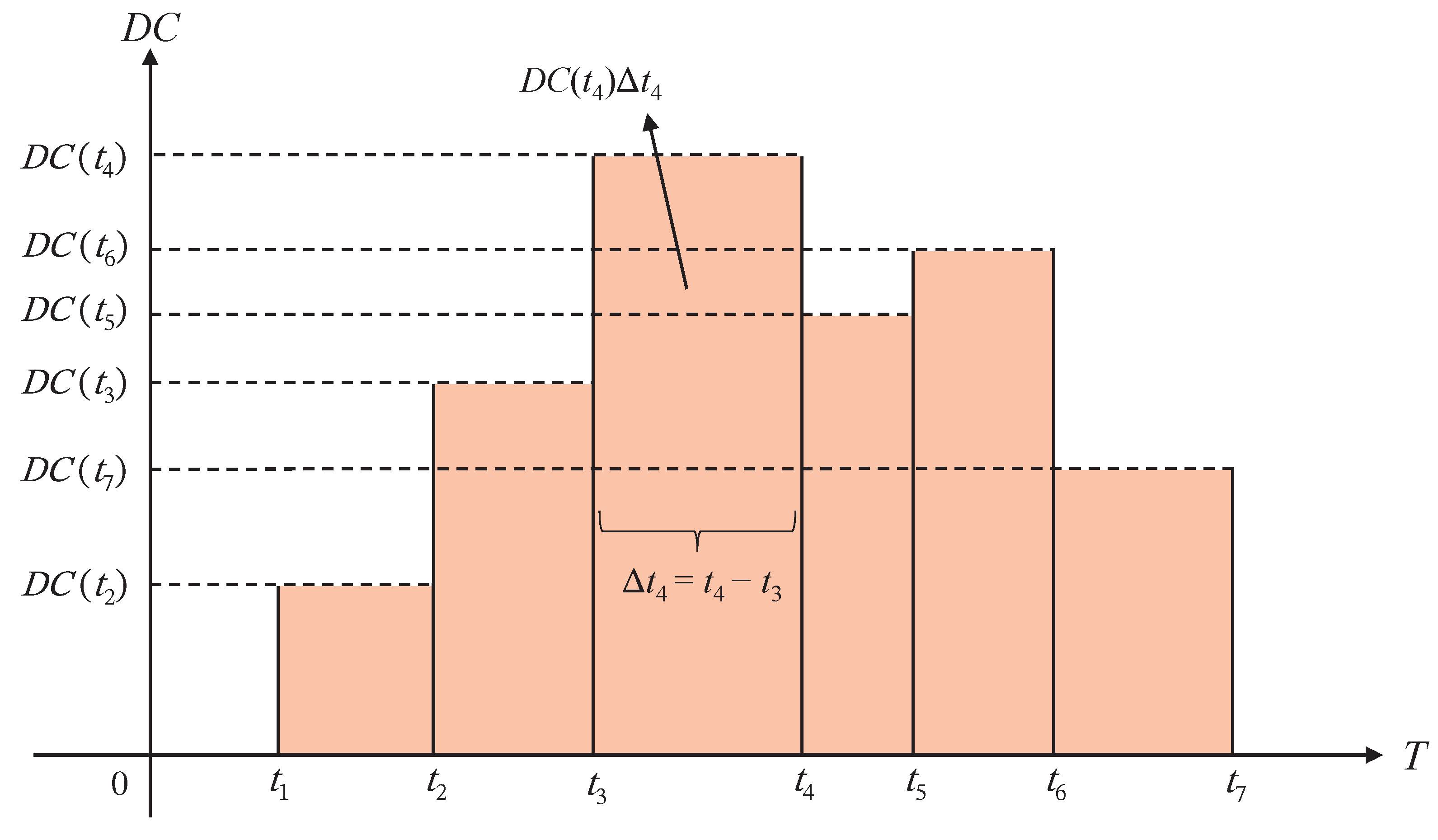
as our dependence measure at the population level. The aggregated statistic ${\omega }_k$ defined in (1) can be naturally interpreted as the area under curve (AUC) after the normalization of $D{C}_k(·)$, and up to the maximum of $\{D{C}_k\left(t_m\right),m=1,2,\dots ,M\}$. Figure 1 provides a geometric view of the statistic ${\omega }_k$. A larger ${\omega }_k$ means a stronger association between $X_k$ and $\mathbf{y}$.

Figure 1. The geometric illustration of LDC statistics. $\Delta t_4$ represents the measurement interval between time points $t_3$ and $t_4$. $DC\left(t_4\right)\Delta t_4$ represents the area of the histogram between time points $t_3$ and $t_4$.

Next, we estimate ${\omega }_k$ in (1). Following Székely et al. [14], given a random sample defined in Section 2.1, we can obtain the estimator of $dCo{v}^2(X_{km},{\mathbf{y}}_m)$ through moment estimation

$${\widehat{dCov}}^2(X_{km},{\mathbf{y}}_m)={\widehat{S}}_1(X_{km},{\mathbf{y}}_m)+{\widehat{S}}_2(X_{km},{\mathbf{y}}_m)-2{\widehat{S}}_3(X_{km},{\mathbf{y}}_m),$$

where ${\widehat{S}}_1(X_{km},{\mathbf{y}}_m)={\displaystyle \frac{1}{n^2}}{\sum }_{i=1}^n{\sum }_{j=1}^n\parallel X_{kim}-X_{kjm}{\parallel }_1{\parallel {\mathbf{y}}_{im}-{\mathbf{y}}_{jm}\parallel }_q$,

${\widehat{S}}_2(X_{km},{\mathbf{y}}_m)={\displaystyle \frac{1}{n^4}}({\sum }_{i=1}^n{\sum }_{j=1}^n\parallel X_{kim}-X_{kjm}{\parallel }_1\left)\right({\sum }_{l=1}^n{\sum }_{f=1}^n\parallel {\mathbf{y}}_{lm}-{\mathbf{y}}_{fm}{\parallel }_q)$,

${\widehat{S}}_3(X_{km},{\mathbf{y}}_m)={\displaystyle \frac{1}{n^3}}{\sum }_{i=1}^n{\sum }_{j=1}^n{\sum }_{l=1}^n\parallel X_{kim}-X_{klm}{\parallel }_1{\parallel {\mathbf{y}}_{jm}-{\mathbf{y}}_{lm}\parallel }_q$. Similarly, ${\widehat{dCov}}^2(X_{km},X_{km})$ and ${\widehat{dCov}}^2({\mathbf{y}}_m,{\mathbf{y}}_m)$ can be defined in the same way. Then, we can get the aggregated estimate of ${\omega }_k$ by

$${\widehat{\omega }}_k=\sum _{m=1}^M{\widehat{DC}}_k\left(t_m\right){\displaystyle \frac{\Delta t_m}{t_M-t_1}}=\sum _{m=1}^M{\displaystyle \frac{{\widehat{dCov}}^2(X_{km},{\mathbf{y}}_m)}{\sqrt{{\widehat{dCov}}^2(X_{km},X_{km}){\widehat{dCov}}^2({\mathbf{y}}_m,{\mathbf{y}}_m)}}}{\displaystyle \frac{\Delta t_m}{t_M-t_1}}.$$

(2)

We refer to the new longitudinal data feature screening procedure based on ${\widehat{\omega }}_k$ as LDCS, which is provided in Algorithm 1. Since we use the sample splitting and data aggregation method, the computational complexity of LDCS can be reduced from $O\left(n^2{M}^2\right)$ to $O\left(n^{2}M\right)$. Finally, we sort ${\widehat{\omega }}_k$ in decreasing order and denote the estimated important predictors set as

$$\widehat{D}=\{1\le k\le p:{\widehat{\omega }}_k\mathrm{is}\mathrm{among}\mathrm{the}\mathrm{top}{d}_0\}$$

by specifying a positive integer, $d_0$. Similarly, we can choose $d_0=a[n/log\left(n\right)]$ with the positive integer $a=1,2,3$ or $d_0=n-1$ [1].

Algorithm 1 Longitudinal distance correlation screening (LDCS).

Input:  source data ${\{{\mathbf{X}}_{im},{\mathbf{y}}_{im},t_m\}}_{m=1}^M$. Output:  $\widehat{D}=\{1\le k\le p:{\widehat{\omega }}_k\mathrm{is}\mathrm{among}\mathrm{the}\mathrm{top}{d}_0\}$.   1: Split the sample into M parts based on the difference of $t_m$.   2: for  $m=1,\dots ,M$ do   3:     for $k=1,\dots ,p$ do   4:          Estimate ${\widehat{S}}_1(X_{km},{\mathbf{y}}_m)$, ${\widehat{S}}_2(X_{km},{\mathbf{y}}_m)$, ${\widehat{S}}_3(X_{km},{\mathbf{y}}_m)$ by moment estimation.   5:          Estimate distance covariance: ${\widehat{dCov}}^2(X_{km},{\mathbf{y}}_m)$, ${\widehat{dCov}}^2(X_{km},X_{km})$, and ${\widehat{dCov}}^2({\mathbf{y}}_m,{\mathbf{y}}_m)$.   6:           Estimate distance correlation: ${\widehat{DC}}_k\left(t_m\right)={\displaystyle \frac{{\widehat{dCov}}^2(X_{km},{\mathbf{y}}_m)}{\sqrt{{\widehat{dCov}}^2(X_{km},X_{km}){\widehat{dCov}}^2({\mathbf{y}}_m,{\mathbf{y}}_m)}}}$.   7:     end for   8: end for    9: for  $k=1,\dots ,p$ do        Estimate the longitudinal distance correlation: ${\widehat{\omega }}_k={\sum }_{m=1}^M{\widehat{DC}}_k\left(t_m\right){\displaystyle \frac{\Delta t_m}{t_M-t_1}}$.   10: end for    11: Sort $\{{\widehat{\omega }}_k,1\le k\le p\}$ in descending order.   12: Obtain the estimated important predictors set $\widehat{D}$.

Next, we analyze the properties of LDCS. We should make the following distribution assumption.

(C.1):

Both q-dimensional vector $\mathbf{y}$ and p-dimensional vector $\mathbf{X}$ have a sub-exponential tail probability uniformly in p, meaning that there exists constant $b_0>0$, such that, for all $0<b\le b_0$,

$$\underset{t}{sup}{E\{exp(2b\parallel \mathbf{y}\parallel }_q^2\left|t\right\}<\infty ,\mathrm{and}\underset{t}{sup}\underset{1\le k\le p}{max}E\{exp(2b\parallel X_k{\parallel }_1^2\left|t\right\}<\infty .$$

Remark 1. 

Assumption (C.1) is frequently utilized in technical proofs for ultra-high-dimensional problems, such as those in Liu [3] and Li et al. [7], as it concerns the moments of the response and predictors. Any bounded or normal distribution would satisfy this assumption.

We present the asymptotic properties of LDCS as follows.

Theorem 1 

(Sure screening property). Under Assumption (C.1), for any $0\le \tau <1/2$ and $0<\kappa <{\displaystyle \frac{1}{2}}-\tau$, there exist constants $c_1>0$, $c_2>0$, and $c_3>0$, such that

$$Pr\left\{\underset{1\le k\le p}{max}|{\widehat{\omega }}_k-{\omega }_k|\ge c_1{n}^{-\tau }\right\}\le O\left\{p\left[exp\left(-c_2{n}^{1-2(\tau +\kappa )}\right)+nexp(-c_3{n}^{\kappa })\right]\right\}.$$

(3)

Furthermore, with ${min}_{k\in D}{\omega }_k\ge 2c_1{n}^{-\tau }$ being supposed, then

$$Pr\left\{D\subseteq \widehat{D}\right\}\ge 1-O\left\{L_0\left[exp\left(-c_2{n}^{1-2(\tau +\kappa )}\right)+nexp\left(-c_3{n}^{\kappa }\right)\right]\right\},$$

(4)

where $L_0$ is the cardinality of D.

Theorem 1 shows that LDCS can effectively identify important predictors for the response. In addition, if we select the optimal order $\kappa =(1-2\tau )/3$, then Equation (3) becomes

$$Pr\left\{\underset{1\le k\le p}{max}\left|{\widehat{\omega }}_k-{\omega }_k\right|\ge c_1{n}^{-\tau }\right\}\le O\left\{pexp\left(-c_2{n}^{(1-2\tau )/3}\right)\right\}.$$

Theorem 2 

(Rank consistency property). Under Assumption (C.1), supposing ${min}_{k\in D}{\omega }_k-{max}_{k\in D^c}{\omega }_k\ge 2c_4{n}^{-\tau }$ for constant $c_4>0$ and $0\le \tau <1/2$, $0<\kappa <{\displaystyle \frac{1}{2}}-\tau$, there exist constants $c_5>0$ and $c_6>0$, such that

$$Pr\left\{\underset{k\in D}{min}{\widehat{\omega }}_k-\underset{k\in D^c}{max}{\widehat{\omega }}_k>0\right\}>1-O\left\{p\left[exp\left(-c_5{n}^{1-2(\tau +\kappa )}\right)+nexp\left(-c_6{n}^{\kappa }\right)\right]\right\}.$$

(5)

Furthermore, as discussed in Theorem 1, if $logp=o\left\{n^{(1-2\tau )/3}\right\}$, then

$${liminf}_{n\to \infty }\left(\underset{k\in D}{min}{\widehat{\omega }}_k-\underset{k\in D^c}{max}{\widehat{\omega }}_k\right)>0,\mathit{almost}\mathit{surely}.$$

Appendix A gives the technical proofs of Theorems 1 and 2.

Remark 2. 

Theorem 1 is essential for all ultra-high-dimensional data feature screening procedures, as it guarantees that $\widehat{D}$ contains all predictors in D with high probability. Theorem 2 provides a stronger theoretical result, as important predictors are more likely to be ranked higher than unimportant ones. In other words, if we assume $\delta =c_4{n}^{-\tau }$, then with a high probability, there exists a δ that can effectively separate the important and unimportant predictors.

2.3. Conditional Screening Procedure

When there exists a high correlation between predictors, LDCS may incorrectly exclude some truly informative predictors. Wang et al. [15] applied the idea of conditional screening to deal with the problem and obtained excellent theoretical properties. Therefore, we applied this method to deal with the above problem. We denote

$$\mathcal{A}=\{k:F(\mathbf{y}|\mathbf{X},\mathbf{Z})\mathrm{functionally}\mathrm{depends}\mathrm{on}{X}_k,k=1,\dots ,p\}.$$

where $F(\mathbf{y}|\mathbf{X},\mathbf{Z})$ denotes the conditional distribution function of $\mathbf{y}$, given $\mathbf{X}$ and $\mathbf{Z}$.

Wang et al. [15] proposed CDC based on Székely et al. [14] to deal with the issue of DC, which may make serious errors when predictors are highly correlated. For details, given the conditional predictor vector $\mathbf{Z}$, they defined CDC between $\mathbf{y}$ and $\mathbf{X}$ as the square root of

$$cdCo{r}^2(\mathbf{X},\mathbf{y}|\mathbf{Z})={\displaystyle \frac{cdCo{v}^2(\mathbf{X},\mathbf{y}|\mathbf{Z})}{\sqrt{cdCo{v}^2(\mathbf{X},\mathbf{X}|\mathbf{Z})cdCo{v}^2(\mathbf{y},\mathbf{y}|\mathbf{Z})}}},$$

where conditional distance covariance is defined as the square root of

$$cdCo{v}^2(\mathbf{X},\mathbf{y}|\mathbf{Z})={\int }_{R^{p+q}}{\parallel {\varphi }_{\mathbf{X},\mathbf{y}|\mathbf{Z}}(\mathbf{s},\mathbf{t})-{\varphi }_{\mathbf{X}|\mathbf{Z}}\left(\mathbf{s}\right){\varphi }_{\mathbf{y}|\mathbf{Z}}\left(\mathbf{t}\right)\parallel }^{2}p(\mathbf{s},\mathbf{t})d\mathbf{s}d\mathbf{t}.$$

Similar to Section 2.2, we split the longitudinal data into s parts based on the difference of $t_m$, and denote the conditional distance correlation between $X_{km}$ and ${\mathbf{y}}_m$, given ${\mathbf{Z}}_m$ at the mth time point $t_m$, by $CD{C}_k\left(t_m\right)=cdCo{r}^2(X_{km},{\mathbf{y}}_m|{\mathbf{Z}}_m)$. We define

$${\rho }_k=\sum _{m=1}^{M}CD{C}_k\left(t_m\right){\displaystyle \frac{\Delta t_m}{t_M-t_1}}$$

(6)

as our dependence measure given some important predictors $\mathbf{Z}$. We denote $d_{ij,k}^X\left(t_m\right)=d(X_{kim},X_{kjm})$ as the Euclidean distance between $X_{kim}$ and $X_{kjm}$, where $i,j=1,...,n$ at the mth measurement. Similarly, $d_{ij,k}^y\left(t_m\right)$ can be denoted in the same way. Then, the distance function can be defined as

$$d_{ijlf,k}^{\prime }\left(t_m\right)={\displaystyle \frac{d_{ijlf,k}\left(t_m\right)+d_{ijfl,k}\left(t_m\right)+d_{iflj,k}\left(t_m\right)}{3}},$$

where $d_{ijlf,k}\left(t_m\right)=(d_{ij,k}^X\left(t_m\right)+d_{lf,k}^X\left(t_m\right)-d_{il,k}^X\left(t_m\right)-d_{jf,k}^X\left(t_m\right))(d_{ij,k}^y\left(t_m\right)+d_{lf,k}^y\left(t_m\right)-d_{il,k}^y\left(t_m\right)-d_{jf,k}^y\left(t_m\right))$. Note that $d_{ijfl,k}\left(t_m\right)$ and $d_{iflj,k}\left(t_m\right)$ are defined similarly. Let ${\omega }_{im}\left({\mathbf{Z}}_m\right)=K(({\mathbf{Z}}_{im}-{\mathbf{Z}}_m)/\mathbf{H})$ and ${\omega }_m\left({\mathbf{Z}}_m\right)={\sum }_i^n{\omega }_{im}\left({\mathbf{Z}}_m\right)$, where H is a diagonal matrix determined by bandwidth h, selected using the plug-in method. $K(·)$ is a kernel function, which is set as the Gaussian kernel function in this paper, i.e.,

$$K_H(\mathbf{Z})={\left|H\right|}^{-1}K(H^{-1}\mathbf{Z})={\left(2\pi \right)}^{-r/2}{\left|H\right|}^{-1}exp(-{\displaystyle \frac{1}{2}}{\mathbf{Z}}^{\prime }{H}^{-2}\mathbf{Z}).$$

Given ${\mathbf{Z}}_m$, the sample conditional distance covariance

$${\widehat{cdCov}}^2(X_{km},{\mathbf{y}}_m|{\mathbf{Z}}_m)={\displaystyle \frac{1}{n^4}}\sum _{i,j,l,f}{\psi }_n({\mathbf{W}}_{im},{\mathbf{W}}_{jm},{\mathbf{W}}_{lm},{\mathbf{W}}_{fm};{\mathbf{Z}}_m)),$$

where

$${\psi }_n({\mathbf{W}}_{im},{\mathbf{W}}_{jm},{\mathbf{W}}_{lm},{\mathbf{W}}_{fm};{\mathbf{Z}}_m)={\displaystyle \frac{n^4{\omega }_{im}\left({\mathbf{Z}}_m\right){\omega }_{jm}\left({\mathbf{Z}}_m\right){\omega }_{lm}\left({\mathbf{Z}}_m\right){\omega }_{fm}\left({\mathbf{Z}}_m\right)}{4{\omega }^4\left({\mathbf{Z}}_m\right)}}{d}_{ijlf,k}^{\prime }\left(t_m\right).$$

The sample conditional distance covariances ${\widehat{cdCov}}^2(X_{km},X_{km}|{\mathbf{Z}}_m)$ and ${\widehat{cdCov}}^2({\mathbf{y}}_m,{\mathbf{y}}_m|{\mathbf{Z}}_m)$ can be estimated similarly. Thus, the plug-in estimate of $CD{C}_k\left(t_m\right)$ is

$${\widehat{CDC}}_k^{\ast }\left(t_m\right)={\displaystyle \frac{1}{n}}\sum _{i=1}^n{\displaystyle \frac{{\widehat{cdCov}}^2(X_{kim},{\mathbf{y}}_{im}|{\mathbf{Z}}_{im})}{\sqrt{{\widehat{cdCov}}^2(X_{kim},X_{kim}|{\mathbf{Z}}_{im}){\widehat{cdCov}}^2({\mathbf{y}}_{im},{\mathbf{y}}_{im}|{\mathbf{Z}}_{im})}}},$$

and the aggregated estimate of ${\rho }_k$ is

$${\widehat{\rho }}_k^{\ast }=\sum _{m=1}^M{\widehat{CDC}}_k^{\ast }\left(t_m\right){\displaystyle \frac{\Delta t_m}{t_M-t_1}}.$$

(7)

Based on ${\widehat{\rho }}_k^{\ast }$, we propose a conditional screening procedure, specifically designed to handle highly correlated predictors:

$$\widehat{\mathcal{A}}=\{1\le k\le p:{\widehat{\rho }}_k^{\ast }\mathrm{is}\mathrm{among}\mathrm{the}\mathrm{top}{d}_0\}.$$

We refer to the new method as LCDCS. Similar to LDCS, the computational complexity of LCDCS can be reduced from $O\left(n^3{M}^3\right)$ to $O\left(n^{3}M\right)$.

Before proving the asymptotic properties of LCDCS, we list the other technical assumptions:

(C.2):

The kernel function $K(·)$ is uniformly bounded and satisfies the following conditions: $K\left(u\right)\ge 0$, $\int K\left(u\right)du=1$, $\int uK\left(u\right)du=0$, and ${\int \parallel u\parallel }^{2}K\left(u\right)du<\infty$.

(C.3):

If $Z_1,Z_2,Z_3,Z_4$ are independent copies of Z, and then, for $1\le k\le p$, there exists constant $C>0$, such that

$$\underset{k}{sup}|E\left\{d_{1234,k}\right|Z_1,Z_2,Z_3,Z_4\}-E\left\{d_{1234,k}\right|Z_1^{\prime },Z_2,Z_3,Z_4\}|\le C|Z_1-Z_1^{\prime }|.$$

We present the asymptotic properties of LCDCS as follows.

Theorem 3 

(Sure screening property). Under Assumption (C.1)–(C.3), if the bandwidth for kernel estimation of $\mathbf{Z}$ satisfies $h=O\left\{n^{-\tilde{\tau }/\left(2r\right)}\right\}$, where r is the dimension of $\mathbf{Z}$, then for any $0\le \tilde{\tau }<1/2$ and $0<\tilde{\kappa }<1/2-\tilde{\tau }$, there exist constants $c_7>0$, $c_8>0$ and $c_9>0$, such that

$$Pr\left\{\underset{1\le k\le p}{max}|{\widehat{\rho }}_k^{\ast }-{\rho }_k|\ge c_7{n}^{-\tilde{\tau }}\right\}\le O\left\{p\left[exp\left(-c_8{n}^{1-2(\tilde{\tau }+\tilde{\kappa })}\right)+n^{4}exp(-c_9{n}^{\tilde{\kappa }})\right]\right\}.$$

(8)

Furthermore, supposing ${min}_{k\in \mathcal{A}}{\rho }_k\ge 2c_7{n}^{-\tilde{\tau }}$, then

$$Pr\left\{\mathcal{A}\subseteq \widehat{\mathcal{A}}\right\}\ge 1-O\left\{L_1\left[exp\left(-c_8{n}^{1-2(\tilde{\tau }+\tilde{\kappa })}\right)+n^{4}exp\left(-c_9{n}^{\tilde{\kappa }}\right)\right]\right\},$$

(9)

where $L_1$ is the cardinality of $\mathcal{A}$. If we set $\tilde{\kappa }=(1-2\tilde{\tau })/3$, then the first part of Theorem 3 becomes

$$Pr\left\{\underset{1\le k\le p}{max}\left|{\widehat{\rho }}_k^{\ast }-{\rho }_k\right|\ge c_7{n}^{-\tilde{\tau }}\right\}\le O\left\{pexp\left(-c_8{n}^{(1-2\tilde{\tau })/3}\right)\right\}.$$

Theorem 4 

(Rank consistency property). Under Assumption (C.1)–(C.3), supposing ${min}_{k\in D}{\rho }_k-{max}_{k\in D^c}{\rho }_k\ge 2c_{10}{n}^{-\tilde{\tau }}$ for constant $c_{10}>0$ and $0\le \tilde{\tau }<1/2$, $0<\tilde{\kappa }<{\displaystyle \frac{1}{2}}-\tilde{\tau }$, there exist constants $c_{11}>0$ and $c_{12}>0$, such that

$$Pr\left\{\underset{k\in D}{min}{\widehat{\rho }}_k^{\ast }-\underset{k\in D^c}{max}{\widehat{\rho }}_k^{\ast }>0\right\}>1-O\left\{p\left[exp\left(-c_{11}{n}^{1-2(\tilde{\tau }+\tilde{\kappa })}\right)+n^{4}exp\left(-c_{12}{n}^{\tilde{\kappa }}\right)\right]\right\}.$$

(10)

Furthermore, as discussed in Theorem 3, if $logp=o\left\{n^{(1-2\tilde{\tau })/3}\right\}$, then

$${liminf}_{n\to \infty }\left(\underset{k\in \mathcal{A}}{min}{\widehat{\rho }}_k^{\ast }-\underset{k\in {\mathcal{A}}^c}{max}{\widehat{\rho }}_k^{\ast }\right)>0,\mathit{almost}\mathit{surely}.$$

Appendix A gives the technical proofs of Theorems 3 and 4.

3. Results

3.1. Simulation Study

We conduct several simulated examples to evaluate the screening performance of LDCS and LCDCS, and compare the results with those of some existing methods, including partial residual sure independence screening (PRSIS) [3], time-varying coefficient models’ sure independence screening (TVCM-SIS) [19], distance correlation sure independence screening (DC-SIS) [7], conditional distance correlation sure independence screening (CDC-SIS) [9], and covariate information number sure independence screening (CIS) [10]. PRSIS and TVCM-SIS are longitudinal data feature screening procedures where PRSIS is based on partially linear models and TVCM-SIS is based on time-varying coefficient models. DC-SIS, CDC-SIS, and CIS are all model-free methods for cross-sectional data.

We repeat each simulation example 500 times. In all examples, the number of predictors is $p=2000$, and the sample size is $n=80$, yielding a submodel size of $d_0=\left[n/log\left(n\right)\right]=18$. The predictor ${\mathbf{X}}_{ki}(k=1,\dots ,p)$ and the random error ${ϵ}_i$ are generated independently from $\mathbf{MVN}(\mathbf{0},{\sigma }_0^2\Sigma )$, where ${\sigma }_0$ and $\Sigma$ are different in each example. The time points $t_1,...,t_M$ are sampled from a standard uniform distribution and do not change in a simulation. We use the following four criteria to assess the screening performance:

• $MMS$: The minimum submodel size containing all important predictors. The median and robust standard deviation (RSD = IQR/1.34) of $MMS$ are reported, where IQR denotes interquartile range.
• $P_k$: The proportion of the important predictor $X_k$ selected in the submodel.
• $P_a$: The proportion of all important predictors selected in the submodel.
• $d_c$: The average number of important predictors selected in the submodel.

3.1.1. Example 1: Partially Linear Models

We generate the response from the following two models:

Model (1.a): $y_{im}={\beta }_1{X}_{1im}+{\beta }_2{X}_{2im}+{\beta }_3{X}_{3im}+{\beta }_{4}I(X_{4im}>0)+f\left(t_m\right)+{ϵ}_{im},$

Model (1.b): $y_{im}={\beta }_1{\beta }_2{X}_{1im}{X}_{2im}+{\beta }_3{X}_{3im}+{\beta }_4{X}_{4im}+f\left(t_m\right)+{ϵ}_{im}.$

Model (1.a) considers categorical predictor variables, while Model (1.b) incorporates interaction effects. These two models are based on Model (1.a) and Model (1.b) in Li et al. [7], but the difference is that we introduced longitudinal measurements and nonlinear time variables. We set ${({\beta }_1,{\beta }_2,{\beta }_3,{\beta }_4)}^T={(-1,-0.75,1,4)}^T$, $f\left(t\right)=36sin\left(4\pi t\right)$ and ${\sigma }_0=2$ in Model (1.a), and ${({\beta }_1,{\beta }_2,{\beta }_3,{\beta }_4)}^T={(-2.25,-2,-1,1)}^T$, $f\left(t\right)=4sin\left(2\pi t\right)$, and ${\sigma }_0=1$ in Model (1.b). Furthermore, we set the repeated measurements $M_i\equiv 5$ and the within-subject correlation structure as first-order autoregressive (AR(1)) structure. The within-subject correlations are set to $\rho =0.3$ and $0.6$ for each model, respectively.

The detailed results are reported in Table 1. For the four different situations, our proposed method LDCS achieves the smallest MMS (including median and RSD), along with the largest $P_a$ and $d_c$. When a strong nonlinear time effect is present, the model-free feature screening procedures DC-SIS and CIS perform less effectively. Furthermore, we observe that TVCM-SIS and PRSIS are not as effective in identifying interaction effects. While CIS relatively successfully identifies interaction effects, it tends not to retain important predictors with and without interaction effects simultaneously. Example 1 demonstrates that our proposed method LDCS is unaffected by strong time effects and performs better in handling situations with interaction effects in partially linear models.

Table 1. $MMS$, $P_k$, $P_a$, $d_c$ for Example 1.

Method	MMS		${\mathit{P}}_{\mathit{k}}$				${\mathit{P}}_{\mathit{a}}$	${\mathit{d}}_{\mathit{c}}$
	Median	RSD	${\mathit{P}}_{\mathit{1}}$	${\mathit{P}}_{\mathit{2}}$	${\mathit{P}}_{\mathit{3}}$	${\mathit{P}}_{\mathit{4}}$
	Model (1.a), ${\rho }_1=0.3$
LDCS	4.00	0.00	1.00	0.99	1.00	1.00	0.99	3.99
TVCM-SIS	4.00	3.73	0.99	0.86	0.99	0.98	0.82	3.82
PRSIS	4.00	82.28	0.84	0.74	0.84	0.83	0.68	3.25
DC-SIS	370.00	356.90	0.31	0.17	0.33	0.27	0.04	1.08
CIS	609.50	726.49	0.34	0.13	0.38	1.00	0.04	1.85
	Model (1.a), ${\rho }_1=0.6$
LDCS	4.00	0.00	1.00	0.96	1.00	1.00	0.96	3.96
TVCM-SIS	4.00	4.48	0.99	0.84	0.98	0.99	0.81	3.80
PRSIS	4.00	23.51	0.89	0.78	0.90	0.90	0.71	3.47
DC-SIS	302.50	349.63	0.43	0.17	0.46	0.39	0.08	1.45
CIS	667.00	711.38	0.35	0.13	0.33	1.00	0.04	1.82
	Model (1.b), ${\rho }_1=0.3$
LDCS	13.00	22.57	0.90	0.90	0.83	0.82	0.59	3.45
TVCM-SIS	651.00	626.12	0.26	0.21	0.81	0.81	0.03	2.08
PRSIS	1022.50	773.51	0.14	0.11	0.93	0.90	0.01	2.08
DC-SIS	19.00	33.58	0.75	0.75	0.87	0.86	0.49	3.23
CIS	490.50	596.08	0.87	0.89	0.18	0.17	0.02	2.10
	Model (1.b), ${\rho }_1=0.6$
LDCS	21.00	38.81	0.87	0.84	0.77	0.79	0.46	3.26
TVCM-SIS	587.50	672.57	0.22	0.23	0.72	0.74	0.02	1.91
PRSIS	957.00	787.13	0.15	0.12	0.80	0.84	0.00	1.91
DC-SIS	30.00	47.95	0.64	0.64	0.83	0.83	0.36	2.93
CIS	523.00	608.02	0.89	0.89	0.17	0.16	0.03	2.10

3.1.2. Example 2: Time-Varying Coefficient Models

In this example, we generate the response from the following two models:

Model (2.a): $y_{im}={\beta }_1\left(t_m\right)X_{1im}+{\beta }_2\left(t_m\right)X_{2im}+{\beta }_3\left(t_m\right)X_{3im}+{\beta }_4\left(t_m\right)X_{4im}+{ϵ}_{im},$

Model (2.b): $log\left({\mu }_i\left(t_m\right)\right)={\beta }_1\left(t_m\right)X_{1im}+{\beta }_2\left(t_m\right)X_{2im}+{\beta }_3\left(t_m\right)X_{3im}+{\beta }_4\left(t_m\right)X_{4im}.$

Model (2.a) is similar to Example I in Chu et al. [19], but we set a smaller sample size and measurements. Model (2.b) considers a count response with Poisson distribution, which is based on Example II in Chu et al. [20], but we use time-varying coefficient model, rather than the generalized varying coefficient mixed-effect model. In Model (2.a), we set ${\beta }_1\left(t\right)=-4cos\left(4\pi t\right)I(t<0.5)$, ${\beta }_2\left(t\right)=-4.25sin\left(4\pi t\right)I(t<0.5)$, ${\beta }_3\left(t\right)=sin\left(4\pi t\right)$, ${\beta }_4\left(t\right)=1.25(1.2-t)$ and ${\sigma }_0=2$. In Model (2.b), we set ${\beta }_1\left(t\right)=-sin\left(2\pi t\right)$, ${\beta }_2\left(t\right)=-1.25sin\left(2\pi t\right)$, ${\beta }_3\left(t\right)=sin\left(2\pi t\right)$, ${\beta }_4\left(t\right)=1.25sin\left(2\pi t\right)$, and ${\sigma }_0=1$. Furthermore, we set the within-subject correlation structure as a compound symmetry (CS) structure. The within-subject correlations are set to $\rho =0.3$ and $0.6$ for each model, respectively.

Table 2 presents the detailed simulation results for Example 2. It can be seen that the results of Example 2 are similar to those of Example 1, i.e., our proposed method LDCS achieves the smallest MMS (including median and RSD), along with the largest $P_a$ and $d_c$. Specifically, for Model (2.a), although TVCM-SIS is based on the assumption of varying coefficient models, its performance is not ideal when the categorical predictors have a stronger impact on the response. For Model (2.b), the screening performance of TVCM-SIS, PRSIS, DC-SIS, and CIS is all unsatisfactory, indicating that these methods are not well suited for varying coefficient models with count responses. These examples further demonstrate that, for some special varying coefficient models, our proposed method LDCS may achieve better screening performance.

Table 2. $MMS$, $P_k$, $P_a$, $d_c$ for Example 2.

Method	MMS		${\mathit{P}}_{\mathit{k}}$				${\mathit{P}}_{\mathit{a}}$	${\mathit{d}}_{\mathit{c}}$
	Median	RSD	${\mathit{P}}_{\mathit{1}}$	${\mathit{P}}_{\mathit{2}}$	${\mathit{P}}_{\mathit{3}}$	${\mathit{P}}_{\mathit{4}}$
	Model (2.a), ${\rho }_1=0.3$
LDCS	12.00	93.47	0.84	0.85	0.82	0.94	0.54	3.45
TVCM-SIS	187.00	785.82	0.56	0.57	0.84	0.89	0.36	2.86
PRSIS	740.50	958.58	0.65	0.67	0.23	0.99	0.10	2.54
DC-SIS	335.50	682.46	0.72	0.71	0.32	0.99	0.15	2.74
CIS	948.00	755.78	0.47	0.46	0.20	0.55	0.01	1.68
	Model (2.a), ${\rho }_1=0.6$
LDCS	14.00	105.22	0.84	0.84	0.82	0.95	0.53	3.45
TVCM-SIS	157.50	750.37	0.57	0.57	0.84	0.90	0.38	2.88
PRSIS	753.50	861.19	0.64	0.64	0.19	0.97	0.07	2.44
DC-SIS	366.50	601.87	0.67	0.68	0.27	0.98	0.08	2.61
CIS	1059.00	695.52	0.47	0.46	0.16	0.56	0.01	1.66
	Model (2.b), ${\rho }_1=0.3$
LDCS	16.00	45.52	0.76	0.93	0.75	0.95	0.52	3.39
TVCM-SIS	261.50	638.06	0.34	0.52	0.38	0.53	0.14	1.77
PRSIS	845.00	972.01	0.21	0.34	0.22	0.33	0.05	1.10
DC-SIS	430.00	715.86	0.34	0.50	0.35	0.53	0.18	1.71
CIS	1402.50	537.31	0.05	0.13	0.07	0.14	0.01	0.40
	Model (2.b), ${\rho }_1=0.6$
LDCS	24.50	60.63	0.71	0.91	0.73	0.92	0.45	3.26
TVCM-SIS	395.50	735.63	0.33	0.50	0.35	0.52	0.11	1.70
PRSIS	916.00	921.83	0.18	0.27	0.18	0.31	0.03	0.94
DC-SIS	557.00	816.23	0.30	0.47	0.28	0.50	0.11	1.55
CIS	1423.50	558.58	0.06	0.08	0.05	0.11	0.00	0.30

3.1.3. Example 3: Partially Linear Single-Index Models

We assess the screening performance of LCDCS when the predictors are correlated with each other. The response is generated from Model (3):

Model (3): $y_{im}={({\beta }_1{X}_{1im}+{\beta }_2{X}_{2im}+{\beta }_3{X}_{3im}+{\beta }_4{X}_{4im})}^2+f\left(t_m\right)+{ϵ}_{im},$

We set ${({\beta }_1,{\beta }_2,{\beta }_3,{\beta }_4)}^T={(3,2.5,2.5,3)}^T$, $f\left(t\right)=36t/(1-t)$, ${\sigma }_0=1$, the repeated measurements $M_i\equiv 3$ and the within-subject correlation structure as AR(1) structure with within-subject correlation as ${\rho }_1=0.5$. The correlation structure between predictors is set as CS structure, with two scenarios considered: ${\rho }_2=0.5$ and ${\rho }_2=0.8$.

We first use LDCS and DC-SIS to screen the most relevant predictor as a conditional predictor for LCDCS and CDC-SIS, respectively. Table 3 presents the detailed simulation results for Example 3. It can be seen that our proposed method, LCDCS, also achieves the smallest MMS (including median and RSD), along with the largest $P_a$ and $d_c$. Since the number of repeated measurements is only 3, the improvement in screening performance of LCDCS over CDC-SIS is not particularly obvious. Additionally, the screening performance of TVCM-SIS and PRSIS is very poor, indicating that these methods, which rely on specific model assumptions, may not perform well in some complex model structures. CIS is also not well suited when the predictors are correlated. This example demonstrates that our proposed method, LCDCS, is more suitable for longitudinal data with correlated predictors in some special model structures.

Table 3. $MMS$, $P_k$, $P_a$, $d_c$ for Example 3.

Method	MMS		${\mathit{P}}_{\mathit{k}}$				${\mathit{P}}_{\mathit{a}}$	${\mathit{d}}_{\mathit{c}}$
	Median	RSD	${\mathit{P}}_{\mathit{1}}$	${\mathit{P}}_{\mathit{2}}$	${\mathit{P}}_{\mathit{3}}$	${\mathit{P}}_{\mathit{4}}$
	Model (3), ${\rho }_2$ = 0.5
LCDCS	6.00	8.21	0.97	0.89	0.91	0.96	0.78	3.73
TVCM-SIS	1307.00	508.40	0.05	0.04	0.07	0.06	0.00	0.22
PRSIS	1557.50	456.16	0.02	0.01	0.02	0.02	0.00	0.07
CDC-SIS	9.00	59.51	0.87	0.76	0.75	0.86	0.59	3.24
CIS	263.50	354.10	0.55	0.38	0.43	0.57	0.07	1.93
	Model (3), ${\rho }_2$ = 0.8
LCDCS	9.00	16.60	0.96	0.83	0.88	0.97	0.68	3.64
TVCM-SIS	1479.00	419.40	0.02	0.02	0.02	0.03	0.00	0.10
PRSIS	1579.50	403.92	0.02	0.01	0.02	0.01	0.00	0.05
CDC-SIS	16.50	90.49	0.85	0.72	0.72	0.86	0.51	3.15
CIS	439.50	481.34	0.38	0.27	0.30	0.37	0.01	1.32

3.2. Application to Gut Microbiota Data

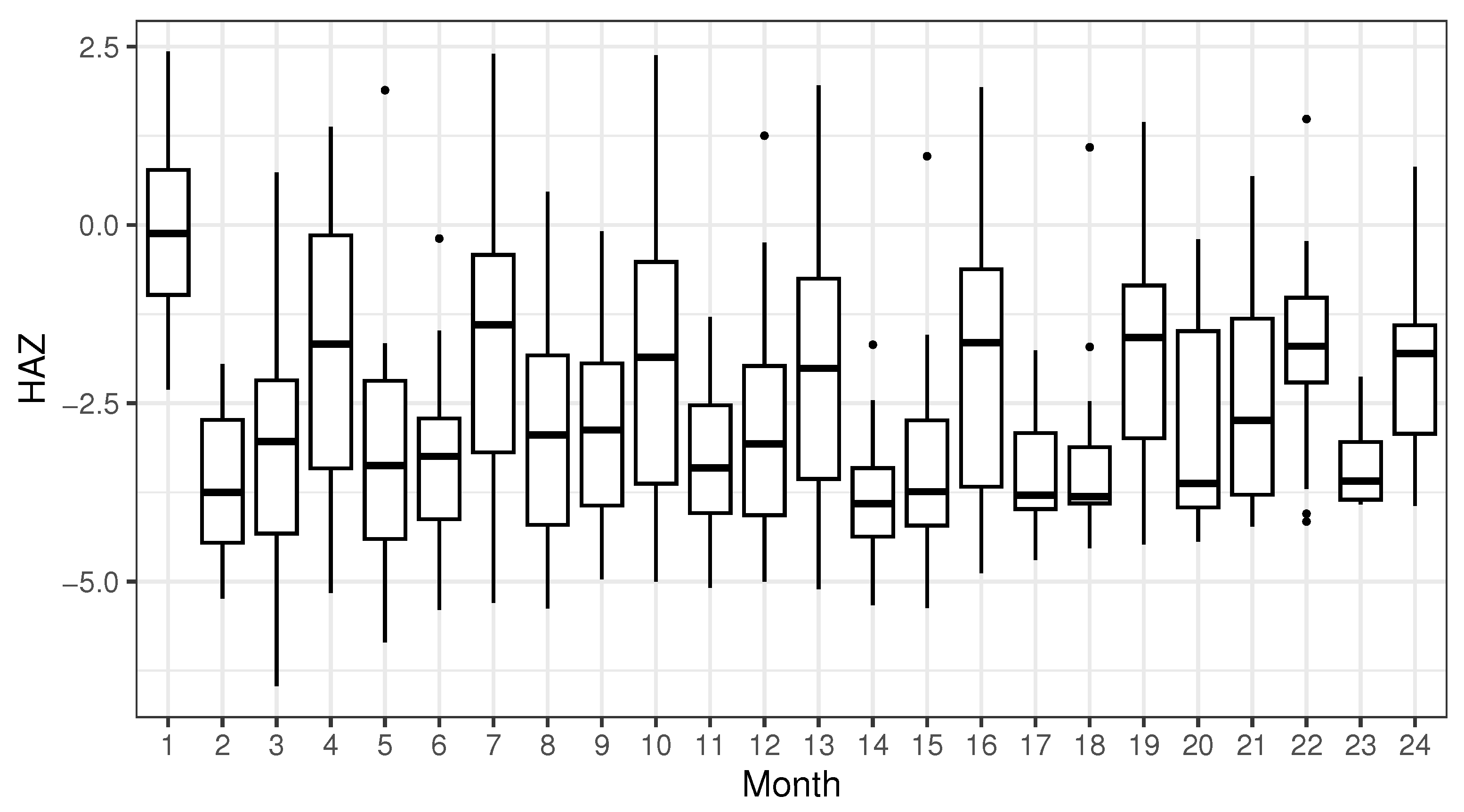
We analyze real-world data to demonstrate the empirical performance of our methods in this section. This is a gut microbiota data from Bangladeshi children, as reported by Subramanian et al. [21]. The longitudinal cohort study aimed at analyzing the effects of therapeutic foods on children. For details, they monitored the growth and development of $n=50$ infants over a two-year period after birth, ultimately collecting a total of $N=996$ fecal samples. Each sample contained 79,597 operational taxonomic units sharing at least $97\%$ nucleotide sequence identity (97%-identity OTUs). Following Subramanian et al. [21], we obtain 1222 97%-identity OTUs that have at least two fecal samples with an average relative abundance greater than 0.1%. In this article, we consider height-for-age Z-scores (HAZ) as the response, which reflects how a child’s height compares to the average height of the same age and gender group, indicating whether growth and development are within the normal range. The HAZ of each child was measured between 6 and 22 times, as illustrated in Figure 2. As a further preprocessing step, we retain only the months in which at least 24 children had their HAZ measured. Thus, we eventually work with a dataset comprising 1222 97%-identity OTUs (the predictors) and HAZ (the response), measured on $n=50$ children over 13 months, for a total of 433 measurements. On this dataset, we apply our LDCS and LCDCS, along with TVCM-SIS, PRSIS, DC-SIS, CDC-SIS, and CIS for feature screening, and we compare the results with those of Subramanian et al. [21].

Figure 2. Trajectories of HAZ in the first 2 years after birth for 50 children. Each boxplot illustrates the variability in the HAZ of children for the given month.

First, we compare the top $d_0=10$ 97%-identity OTUs selected by each method, as summarized in Table 4. Our methods, LDCS and LCDCS, demonstrate a moderate overlap in the number of selected 97%-identity OTUs with PRSIS, DC-SIS, and CDC-SIS, while the selection results of TVCM-SIS and CIS differ significantly from those of the other methods. Next, we compare the top $d_0=220$ 97%-identity OTUs, as Subramanian et al. [21] identified 220 gut microbiota that were significantly different between severe acute malnutrition (SAM) and healthy children. It is obvious that LDCS and LCDCS have the maximum number of 97%-identity OTUs, which align with those of Subramanian et al. [21] among all screening procedures.

Table 4. Number of overlapping 97%-identity OTUs among the top $d_0=10$ (above diagonal) and the top $d_0=220$ (below diagonal) selected via different methods.

		LDCS	LCDCS	TVCM-SIS	PRSIS	DC-SIS	CDC-SIS	CIS
		${\mathit{d}}_{\mathbf{0}}\mathbf{=}\mathbf{10}$
LDCS	$d_0=220$	-	5	0	6	5	7	0
LCDCS		186	-	0	4	2	5	0
TVCM-SIS		94	103	-	0	0	0	1
PRSIS		114	97	70	-	8	8	0
DC-SIS		115	100	69	181	-	6	0
CDC-SIS		118	110	64	160	152	-	0
CIS		35	38	62	52	47	35	-
ANOVA *		103	108	51	47	49	74	45

* Subramanian et al. [21] used an analysis of variance with LMM to identify 97%-identity OTUs that were significantly different between SAM and healthy children.

Furthermore, we evaluate the screening performance through regression analysis. Following Chu et al. [19], we establish time-varying coefficient models with different numbers of 97%-identity OTUs and use the total heritability commonly used in genetic analysis to assess the goodness of fit. The total heritability of all 97%-identity OTUs is calculated through

$$H\left(\mathrm{HAZ}\right)={\displaystyle \frac{\mathit{RSS}\left(\mathrm{HAZ}\right|\mathrm{Fetal})}{\mathit{RSS}\left(\mathrm{HAZ}\right|\mathrm{Fetal})}}-{\displaystyle \frac{\mathit{RSS}\left(\mathrm{HAZ}\right|\mathrm{Fetal},{\mathrm{OTU}}_1,\dots ,{\mathrm{OTU}}_{\mathrm{p}})}{\mathit{RSS}\left(\mathrm{HAZ}\right|\mathrm{Fetal})}}.$$

Here, fetal means whether the child is a singleton birth and RSS is the residual sum of squares defined as

$$RSS=\sum _{i=1}^n\sum _{m=1}^{M_i}{\left(y_i\left(t_{im}\right)-{\widehat{y}}_i\left(t_{im}\right)\right)}^2,$$

where $y_i\left(t_{im}\right)$ denotes the actual value, and ${\widehat{y}}_i\left(t_{im}\right)$ denotes the predicted value from the time-varying coefficient models.

We calculate the total heritability of the top $d_0=1$ to 49 97%-identity OTUs and remove more irrelevant 97%-identity OTUs using forward regression to achieve better regression fitting results. Our proposed method, LCDCS, has the highest total heritability at 64.76%, followed by LDCS with 60.24%. The final number of 97%-identity OTUs selected and the total heritability for each method are shown in Table 5.

Table 5. Quantity of 97%-identity OTUs selected and total heritability for each method.

Method	Number of 97%-Identity OTUs	Total Heritability
LDCS	36	60.24%
LCDCS	39	64.76%
TVCM-SIS	39	49.56%
PRSIS	40	52.77%
DC-SIS	34	51.46%
CDC-SIS	41	55.85%
CIS	41	37.02%

We also plot the curves of total heritability for the different screening procedures, as shown in Figure 3. We note that, overall, when the number of 97%-identity OTUs selected is between 4 and 23, the total heritability of LCDCS is higher than that of other screening procedures. Additionally, when the number of 97%-identity OTUs selected is between 24 and 33, the LDCS method shows a higher total heritability. Therefore, when the number of selected 97%-identity OTUs is moderate, we recommend using LCDCS, while for a larger number of selected 97%-identity OTUs, we recommend using LDCS.

Figure 3. Curves of total heritability with number of 97%-identity OTUs selected through different methods.

We also calculate the heritability of each 97%-identity OTU, which depends on the sequence of selection in the forward regression. The heritability of the kth 97%-identity OTU is calculated through

$$\begin{array}{cc}\hfill H\left({\mathrm{OTU}}_k\right)=& {\displaystyle \frac{RSS\left(\mathrm{HAZ}\right|\mathrm{Fetal},{\mathrm{OTU}}_{\left(1\right)},\dots ,{\mathrm{OTU}}_{(\mathrm{k}-1)})}{RSS\left(\mathrm{HAZ}\right|\mathrm{Fetal})}}\hfill \\ & -{\displaystyle \frac{RSS\left(\mathrm{HAZ}\right|\mathrm{Fetal},{\mathrm{OTU}}_{\left(1\right)},\dots ,{\mathrm{OTU}}_{(\mathrm{k}-1)},{\mathrm{OTU}}_{\left(\mathrm{k}\right)})}{RSS\left(\mathrm{HAZ}\right|\mathrm{Fetal})}}.\hfill \end{array}$$

Table 6 presents the IDs and taxonomic annotations of the top 10 97%-identity OTUs based on the heritability, as selected via LCDCS. The taxonomic annotations are given by Subramanian et al. [21], representing the genus of the gut microbiota. Among the 10 gut microbiota, 4 gut microbiota belong to the Bifidobacterium genus. Bifidobacterium is a common group of probiotics found primarily in the human gut, particularly in infants, and it has been shown to be closely associated with children’s nutrient absorption and growth development. Furthermore, there are 5 97%-identity OTUs that differ from the results of Subramanian et al. [21], which may represent a new discovery. We also perform a sensitivity analysis to evaluate how the parameter $d_0$ influences the empirical results, with detailed information provided in Appendix B.

Table 6. IDs and taxonomic annotations of the top 10 97%-identity OTUs selected via LCDCS based on heritability.

Order	ID	Taxonomic Annotation	Heritability
1	New.0.CleanUp.ReferenceOTU89679 *	Collinsella	9.29%
2	561636	Streptococcus	7.54%
3	New.0.ReferenceOTU340 *	Bifidobacterium	4.87%
4	470527	Lactobacillus	4.43%
5	326977 *	Bifidobacterium	4.22%
6	471180 *	Bifidobacterium	3.31%
7	469868	Bifidobacterium	2.76%
8	345575	Lactococcus	2.59%
9	316587 *	Streptococcus	2.23%
10	New.0.ReferenceOTU339	NA †	2.05%

* 97%-identity OTUs discovered in Subramanian et al. [21]. ^† The taxonomic annotation is not provided by Subramanian et al. [21].

4. Discussion

In this article, we improve DC by applying a sample splitting and data aggregation method to achieve better screening performance with longitudinal data. We also make a simple extension of LDCS to deal with the situation where the predictors are correlated. The two methods are capable of handling longitudinal data with unequal numbers of repeated measurements and unequal intervals between repeated measurement time points. Simulation studies indicate that, in some special situations, such as partially linear models with strong time effects or interaction effects, and varying coefficient models with count responses, our proposed method LDCS demonstrates better screening performance. Furthermore, in the situations where predictors are correlated, our proposed method, LCDCS, also achieves better screening performance for some complex structures. Finally, the results of the application show that LDCS and LCDCS achieve better outcomes at different selection scales.

Inevitably, this work encountered some limitations. For instance, we did not consider the treatment of missing data or time-varying confounding. Additionally, both LDCS and LCDCS rely on sub-exponential tail probability assumptions, which may not always hold in practice. The screening performance of LCDCS is sensitive to bandwidth selection, and due to the kernel estimation, its computational burden is higher than that of some other model-free methods.

We plan to deal with the selection of the threshold $d_0$ in LDCS and LCDCS in a future study. Recently, Liu et al. [22] proposed handling this issue from the perspective of false discovery rate (FDR) control by using Model-X knockoff features. Chi et al. [23] applied Model-X knockoff features to the FDR control problem for time series data by using an e-value aggregation method. Therefore, similarly, we could also consider constructing Model-X knockoff features and corresponding knockoff statistics for each measurement time point in longitudinal data, and then aggregate these statistics by using the e-value aggregation method. We expect that this approach will help handle the selection problem of the threshold $d_0$ in LDCS and LCDCS from the perspective of FDR control.

References

1. Fan, J.Q.; Lv, J.C. Sure Independence Screening for Ultrahigh Dimensional Feature Space. J. R. Stat. Soc. B. 2008, 70, 849–911. [Google Scholar] [CrossRef]
2. Song, R.; Yi, F.; Zou, H. On Varying-Coefficient Independence Screening for High-Dimensional Varying-Coefficient Models. Stat. Sinica. 2014, 24, 1735–1752. [Google Scholar] [CrossRef]
3. Liu, J.Y. Feature Screening and Variable Selection for Partially Linear Models with Ultrahigh-Dimensional Longitudinal Data. Neurocomputing 2016, 195, 202–210. [Google Scholar] [CrossRef]
4. Lai, P.; Liang, W.J.; Wang, F.J.; Zhang, Q.Z. Feature Screening of Quadratic Inference Functions for Ultrahigh Dimensional Longitudinal Data. J. Stat. Comput. Sim. 2020, 90, 2614–2630. [Google Scholar] [CrossRef]
5. Jiang, B.Y.; Lv, J.; Li, J.L.; Cheng, M.Y. Robust Model Averaging Prediction of Longitudinal Response with Ultrahigh-Dimensional Covariates. J. R. Stat. Soc. Ser. B Stat. Methodol. 2024, 87, 337–361. [Google Scholar] [CrossRef]
6. Zhu, L.P.; Li, L.X.; Li, R.Z.; Zhu, L.X. Model-Free Feature Screening for Ultrahigh-Dimensional Data. J. Am. Stat. Assoc. 2011, 106, 1464–1475. [Google Scholar] [CrossRef] [PubMed]
7. Li, R.Z.; Zhong, W.; Zhu, L.P. Feature Screening via Distance Correlation Learning. J. Am. Stat. Assoc. 2012, 107, 1129–1139. [Google Scholar] [CrossRef]
8. Shao, X.F.; Zhang, J.S. Martingale Difference Correlation and Its Use in High-Dimensional Variable Screening. J. Am. Stat. Assoc. 2014, 109, 1302–1318. [Google Scholar] [CrossRef]
9. Wen, C.H.; Pan, W.L.; Huang, M.M.; Wang, X.Q. Sure Independence Screening Adjusted for Confounding Covariates with Ultrahigh Dimensional Data. Stat. Sinica. 2018, 28, 293–317. [Google Scholar] [CrossRef]
10. Nandy, D.; Chiaromonte, F.; Li, R.Z. Covariate Information Number for Feature Screening in Ultrahigh-Dimensional Supervised Problems. J. Am. Stat. Assoc. 2022, 117, 1516–1529. [Google Scholar] [CrossRef]
11. Zhang, J.; Liu, Y.Y.; Cui, H.J. Model-Free Feature Screening via Distance Correlation for Ultrahigh Dimensional Survival Data. Stat. Papers. 2021, 62, 2711–2738. [Google Scholar] [CrossRef]
12. Zhong, W.; Qian, C.; Liu, W.J.; Zhu, L.P.; Li, R.Z. Feature Screening for Interval-Valued Response with Application to Study Association between Posted Salary and Required Skills. J. Am. Stat. Assoc. 2023, 118, 805–817. [Google Scholar] [CrossRef]
13. Zhou, T.Y.; Zhu, L.P. Model-Free Feature Screening for Ultrahigh Dimensional Censored Regression. Stat. Comput. 2017, 27, 947–961. [Google Scholar] [CrossRef]
14. Székely, G.J.; Rizzo, M.L.; Bakirov, N.K. Measuring and Testing Dependence by Correlation of Distances. Ann. Stat. 2007, 35, 2769–2794. [Google Scholar] [CrossRef]
15. Wang, X.Q.; Pan, W.L.; Hu, W.H.; Tian, Y.; Zhang, H.P. Conditional Distance Correlation. J. Am. Stat. Assoc. 2015, 110, 1726–1734. [Google Scholar] [CrossRef]
16. Chen, L.P. Feature Screening Based on Distance Correlation for Ultrahigh-Dimensional Censored Data with Covariate Measurement Error. Comput. Stat. 2021, 36, 857–884. [Google Scholar] [CrossRef]
17. Lu, J.; Lin, L. Model-Free Conditional Screening via Conditional Distance Correlation. Stat. Papers. 2020, 61, 225–244. [Google Scholar] [CrossRef]
18. Dai, C.G.; Lin, B.Y.; Xing, X.; Liu, J.S. False Discovery Rate Control via Data Splitting. J. Am. Stat. Assoc. 2023, 118, 2503–2520. [Google Scholar] [CrossRef]
19. Chu, W.H.; Li, R.Z.; Reimherr, M. Feature Screening for Time-Varying Coefficient Models with Ultrahigh-Dimensional Longitudinal Data. Ann. Appl. Stat. 2016, 10, 596–617. [Google Scholar] [CrossRef]
20. Chu, W.H.; Li, R.Z.; Liu, J.Y.; Reimherr, M. Feature Selection for Generalized Varying Coefficient Mixed-Effect Models with Application to Obesity GWAS. Ann. Appl. Stat. 2020, 14, 276–298. [Google Scholar] [CrossRef] [PubMed]
21. Subramanian, S.; Huq, S.; Yatsunenko, T.; Haque, R.; Mahfuz, M.; Alam, M.A.; Benezra, A.; DeStefano, J.; Meier, M.F.; Muegge, B.D.; et al. Persistent Gut Microbiota Immaturity in Malnourished Bangladeshi Children. Nature 2014, 510, 417–421. [Google Scholar] [CrossRef] [PubMed]
22. Liu, W.J.; Ke, Y.; Liu, J.Y.; Li, R.Z. Model-Free Feature Screening and FDR Control with Knockoff Features. J. Am. Stat. Assoc. 2022, 117, 428–443. [Google Scholar] [CrossRef]
23. Chi, C.M.; Fan, Y.Y.; Ing, C.K.; Lv, J.C. High-Dimensional Knockoffs Inference for Time Series Data. J. Am. Stat. Assoc. 2025, 1–24. [Google Scholar] [CrossRef] [PubMed]