Article

Bootstrap Methods for Correcting Bias in WLS Estimators of the First-Order Bifurcating Autoregressive Model

1
Department of Mathematics and Statistics, North Carolina A&T State University, 1601 E. Market Street, Greensboro, NC 27411, USA
2
Department of Mathematics and Statistics, College of Science, Imam Mohammad Ibn Saud Islamic University, Riyadh 11623, Saudi Arabia
3
Department of Applied Statistics and Insurance, Faculty of Commerce, Mansoura University, El Gomhouria St., El Mansoura 1, Dakahlia Governorate 35516, Egypt
4
Department of Quantitative Methods, School of Business, King Faisal University, Al Ahsa 31982, Saudi Arabia
*
Author to whom correspondence should be addressed.
Stats 2025, 8(3), 79; https://doi.org/10.3390/stats8030079
Submission received: 6 August 2025 / Revised: 31 August 2025 / Accepted: 3 September 2025 / Published: 5 September 2025

Abstract

In this study, we examine the presence of bias in weighted least squares (WLS) estimation within the context of first-order bifurcating autoregressive (BAR(1)) models. These models are widely used in the analysis of binary tree-structured data, particularly in cell lineage research. Our findings suggest that WLS estimators may exhibit significant and problematic biases, especially in finite samples. The magnitude and direction of this bias are influenced by both the autoregressive parameter and the correlation structure of the model errors. To address this issue, we propose two bootstrap-based methods for bias correction of the WLS estimator. The paper further introduces shrinkage-based versions of both single and fast double bootstrap bias correction techniques, designed to mitigate the over-correction and under-correction issues that may arise with traditional bootstrap methods, particularly in larger samples. Comprehensive simulation studies were conducted to evaluate the performance of the proposed bias-corrected estimators. The results show that the proposed corrections substantially reduce bias, with the most notable improvements observed at extreme values of the autoregressive parameter. Moreover, the study provides practical guidance for practitioners on method selection under varying conditions.

1. Introduction

The bifurcating autoregressive (BAR) model is extensively used for analyzing binary tree data, as depicted in Figure 1, which often appears in many fields, particularly in cell progression research, including cell lineage (see, e.g., refs. [1,2,3,4]). The BAR(1) model is an extension of the first-order autoregressive AR(1) model and incorporates a distinctive feature: the correlation between observations of two sister cells that share the same mother cell. This model was introduced by [5] to represent cell lineage data. In practical applications, the BAR(1) model is valuable for modeling the progression of single-cell reproduction c.f. [3]. Several studies have addressed the challenges of estimation and inference related to the BAR model; see for example, [5,6,7,8,9,10,11,12,13]. Maximum likelihood (ML) estimators for the model coefficients and the error correlation in the BAR(1) model were proposed by [5], assuming normally distributed errors. Building on this, ref. [8] investigated the asymptotic properties of ML estimators for the BAR(p) model under the assumption of normality of the error distribution. Conversely, ref. [10] explored least squares (LS) estimation for BAR(p) models without assuming any specific error distribution. They developed LS estimators for the BAR model coefficients and derived an asymptotic distribution of these estimators. However, this study does not examine the finite-sample properties of these estimators. Although LS estimators of the BAR model coefficients are unbiased, ref. [13] showed that the finite sample bias of these estimators can potentially lead to inaccurate conclusions. This finding aligns with the common fact that LS estimators for the AR(1) model often exhibit considerable bias, especially when the autoregressive parameter approaches its limits ( ± 1 ) (e.g., ref. [14]).
To address this problem, ref. [13] proposed two techniques for correcting the bias in the LS estimator of the autoregressive parameter within the BAR(1) model. One technique relies on asymptotic linear bias functions, whereas the other employs a bootstrapping method. Their findings demonstrated that both approaches successfully mitigated bias, with the bootstrap bias-correction method being more effective than the asymptotic linear bias function, specifically when the parameter was near the limit ( + 1 ).
A significant issue in the analysis of cell lineage data is the management of the outlying data. Various strategies have been suggested to create robust estimators that reduce the influence of outlying data within the BAR model framework, such as quasi-maximum likelihood estimation techniques (cf., ref. [15,16]). In this context, ref. [12] introduced robust estimators for the BAR(1) model using weighted absolute deviations. They showed that when the weights are constant, the resulting estimator is an L 1 -type, which is resistant to outlying data in the response space and is more efficient than the least squares (LS) estimator when dealing with heavy-tailed error distributions. Conversely, when the weights are random and are influenced by points in the factor space, the weighted L 1 ( WL 1 ) estimator is robust to outlying data in the factor space. Furthermore, they derived the asymptotic distribution of the WL 1 estimator and examined its properties using large samples. In [17], the authors investigated the bias of WL 1 estimators under finite samples and discovered a significant bias. They proposed two bootstrap-based bias-corrected estimators for the WL 1 estimator. These two bootstrap methods effectively reduced the bias present in WL 1 estimators.
In their exploration of random coefficient bifurcating autoregressive processes, ref. [18] investigated the asymptotic properties of WLS estimators for unknown parameters in the first-order bifurcating autoregressive model. By imposing appropriate conditions on immigration and inheritance, they demonstrated the almost sure convergence of these estimators, along with strong law and central limit theorems. This study primarily depends on the vector-valued martingale theorem. However, they did not assess the bias of WLS estimators when dealing with finite sample sizes, such as small or moderate samples.
Unlike [13,17], which focused on correcting the bias in LS and WL 1 estimators of the autoregressive parameter in the BAR(1) model using bootstrap methods, this study addresses an important limitation in their approach. Specifically, their work did not account for the over-correction and under-correction issues that often arise with traditional bootstrap techniques, particularly as sample sizes increase. To overcome this limitation, we introduce shrinkage-based versions of both single and fast double bootstrap bias correction techniques, specifically designed to mitigate these issues. Our study aims to fill this gap in the literature by providing more reliable bias correction methods for BAR(1) models.
In this study, we focused on analyzing the bias present in the WLS estimators for the BAR(1) models. Our results reveal that the WLS estimators for the BAR(1) autoregressive parameter, ϕ 1 , can exhibit a significant bias, especially when dealing with finite samples. To address this problem, we used bootstrapping methods to create bias-corrected WLS estimators. The bias and mean squared error (MSE) of these estimators are evaluated. It is crucial to recognize that reducing bias might lead to increased variance, which may result in a higher mean squared error (MSE) compared with uncorrected estimates [19].
The remainder of this paper is organized as follows. In Section 2, we present an overview of the BAR(1) model and the WLS estimation. Section 3 empirically investigates the bias of the WLS autoregressive estimator in the BAR(1) model. In Section 4, we introduce bias-corrected WLS estimators. Section 5 summarizes the empirical findings, based on Monte Carlo simulations and compares the performance of bias-corrected and uncorrected WLS estimators. Finally, Section 6 concludes the study with a discussion of the key results and suggestions for future research.

2. The BAR(1) Model and WLS Estimation

2.1. The BAR(1) Model

Consider the random variables X 1 , X 2 , , X n , which denote the data on a complete binary tree spanning g generations. The first datum, X 1 , pertains to generation 0, whereas the X 2 i , X 2 i + 1 , , X 2 i + 1 1 data are associated with the 2 i data in generation i, where i = 1 , 2 , , g . The total number of data points is expressed as n = 2 g + 1 1 . The first-order bifurcating autoregressive (BAR(1)) model is defined as
X t = Y t ϕ + ε t , for all t 2 ,
where X t represents the observed value of a quantitative trait at time t, and Y t = [ 1 , X t / 2 ] , with X t / 2 representing the “mother” of X t for all t 2 , and u indicating the greatest integer less than or equal to u. The vector ϕ = [ ϕ 0 , ϕ 1 ] contains the true model parameters: the intercept parameter, ϕ 0 , and the autoregressive parameter, ϕ 1 . These parameters are also known as inherited effect and maternal correlation, respectively. The range of the autoregressive parameter ϕ 1 is ( 1 , 1 ) to ensure that the process remains stationary. The pairs ( ε 2 t , ε 2 t + 1 ) are assumed to be independently and identically distributed (i.i.d.) according to a joint distribution F. Each pair ( ε 2 t , ε 2 t + 1 ) has a zero mean vector and a variance-covariance matrix given by
Σ ε t = 1 θ θ 1 σ 2 ,
where θ denotes the linear correlation between ε 2 t and ε 2 t + 1 , often referred to as the environmental effect or sister-sister correlation due to their shared mother. Additionally, σ 2 represents the error variance.
The rationale behind this correlation structure is based on the assumption that sister cells, especially those in their early developmental stages, are exposed to a common environment. As a result, two distinct types of correlations are anticipated: (i) environmental correlation between sisters, and (ii) maternal correlation stemming from inherited effects from the mother. In contrast, cells that are more distantly related, such as cousins, experience less environmental overlap, which makes it reasonable to assume that their environmental effects are independent.

2.2. WLS Estimation

Ref. [18] introduced WLS estimators for ϕ 0 and ϕ 1 coefficients for the BAR(1) model by minimizing the following dispersion function:
D ( ϕ ) = 1 2 2 t n w X [ t / 2 ] X t Y t ϕ 2 ,
where w ( · ) denotes the weight function. The choice of w ( · ) is crucial in the estimation process. Ref. [18] emphasized that a suitable choice can significantly affect the convergence and accuracy of the estimators of autoregressive processes. Ref. [18] chose w ( · ) = 1 / ( 1 + X [ t / 2 ] 2 ) to ensure that the weights applied to the observations are adjusted based on the data variability. The term X [ t / 2 ] 2 allows the weights to increase with the magnitude of the data, which can help stabilize the estimation process and improve the performance. When w ( · ) = 1 , the estimator is simplified to the conventional LS-norm. Consequently, the estimate ϕ ^ n can be considered an approximate solution to the equation S n = 0 , where S n is defined as S n = 2 t n w t X [ t / 2 ] Y t Y t .
The joint limiting distribution of the WLS estimators of the BAR(1) model coefficients according to [18] and under some regularity conditions is
n ( ϕ ^ WLS ϕ ) d N ( 0 , τ C 1 Σ C 1 ) ,
where τ = σ 2 ( 1 + θ ) , C = E w X [ t / 2 ] Y 1 Y 1 , Σ = E w X [ t / 2 ] Y 1 Y 1 w X [ t / 2 ] . The method of moments estimators for C and Σ are given by
C ^ = 1 n 1 t = 2 n w X [ t / 2 ] 1 n 1 t = 2 n w X [ t / 2 ] X [ t / 2 ] 1 n 1 t = 2 n w X [ t / 2 ] X [ t / 2 ] 1 n 1 t = 2 n w X [ t / 2 ] X [ t / 2 ] 2 ,
Σ ^ = 1 n 1 t = 2 n w 2 X [ t / 2 ] 1 n 1 t = 2 n w 2 X [ t / 2 ] X [ t / 2 ] 1 n 1 t = 2 n w 2 X [ t / 2 ] X [ t / 2 ] 1 n 1 t = 2 n w 2 X [ t / 2 ] X [ t / 2 ] 2 ,
θ ^ = 1 m σ ^ 2 t = 1 m ε ^ 2 t ε ^ 2 t + 1 ,
and
σ ^ 2 = 1 n 3 t = 2 n ε t ^ 2
where m = ( n 1 ) / 2 and ε ^ t = ( X t Y t ϕ ^ ) .

3. Bias in the WLS Estimators for the BAR(1) Model

In this section, we conduct an empirical study utilizing Monte Carlo simulations to evaluate the bias of the WLS estimator for the autoregressive coefficient ϕ 1 , analyzing its variation with ϕ 1 and θ parameters. The simulations adhered to a specific configuration. Completed binary trees of sizes n = 31 , 63 , 127 , and 255 are created for each combination of ϕ 1 = ± ( 0.10 , 0.25 , 0.55 , 0.85 ) and θ = ± ( 0.10 , 0.25 , 0.55 , 0.85 ) , representing a spectrum of maternal and environmental effect correlation levels. The intercept, ϕ 0 , is consistently set to 10 in all simulations. All generated trees begin with the initial observation X 1 randomly drawn from a larger simulated binary tree of size 127. Moreover, all generated trees are assumed to follow a stationary process.
The paired innovation terms ε 2 t , ε 2 t + 1 are modeled as independent and identically distributed bivariate normal random vectors with a mean of zero and heteroscedastic variance-covariance structure. Specifically, the variance increased over time according to σ t = σ t , simulating realistic growth in variability across generations. For each simulation scenario, N = 10 , 000 binary trees are generated, and the WLS estimator ϕ ^ 1 WLS is computed for each tree. To provide a clear overview of the study setup, Table 1 summarizes the simulation configuration.
The empirical bias, absolute relative bias (ARB), variance, and mean squared error (MSE) of ϕ ^ 1 WLS are then evaluated as follows:
BIAS ^ ( ϕ ^ 1 WLS ) = 1 N j = 1 N ϕ ^ 1 WLS , ( j ) ϕ 1 ,
ARB ^ ( ϕ ^ 1 WLS ) = | BIAS ^ ( ϕ ^ WLS ) / ϕ 1 | ,
Var ^ ( ϕ ^ 1 WLS ) = 1 N j = 1 N 1 ϕ ^ 1 WLS , ( j ) ϕ ^ ¯ 1 WLS 2 ,
MSE ^ ( ϕ ^ 1 WLS ) = 1 N j = 1 N ϕ ^ 1 WLS , ( j ) ϕ 1 2 .
In this context, ϕ ^ 1 WLS , ( j ) represents the WLS estimator from each iteration j = 1 , 2 , , N , whereas ϕ ^ ¯ 1 WLS denotes the average across all N iterations.
Figure 2 illustrates the empirical bias and ARB (expressed as a percentage) of ϕ ^ 1 WLS . The findings suggest that the bias of ϕ ^ 1 WLS can be pronounced for different combinations of ϕ 1 and θ , especially when dealing with smaller sample sizes. Notably, the bias is of particular concern when θ is positive and ϕ 1 is greater than 0.5 .
Generally, ϕ ^ 1 WLS tends to underestimate ϕ 1 for values above 0.5 , with the underestimation becoming more pronounced as ϕ 1 approaches + 1 . In addition, the bias appears to have a linear correlation with ϕ 1 . The ARB results further highlight the bias, showing that for small sample sizes ( n = 31 ) and ϕ 1 close to zero (ranging from 0.3 to + 0.3 ), the bias of ϕ ^ WL 1 can vary from 5% to 60% of the actual value of ϕ 1 as θ shifts from 1 to + 1 . For the smallest sample size ( n = 31 ), the relative bias remains significantly large for ϕ 1 values exceeding 0.5 , as long as θ does not approach 1 . Although the bias is still considerable in most scenarios for n = 63 and n = 127 , it becomes negligible with larger sample sizes ( n = 255 ), except when ϕ 1 is near zero (between 0.3 and + 0.3 ) and θ is positive.

4. Bias-Corrected WLS Estimators for the BAR(1) Model

In this section, we present four bootstrap methods aimed at correcting the bias of the WLS estimator ϕ ^ 1 WLS for the autoregressive coefficient ϕ 1 in the BAR(1) model. Specifically, we introduce the traditional single bootstrap bias-corrected version, the traditional fast double bootstrap bias-corrected version, and two additional bias correction methods—single and fast double bootstrap—based on a shrinkage approach.

4.1. Traditional Bootstrap Bias Correction

The model-based bootstrap method is widely used for addressing bias in least squares (LS) estimation of the AR(1) model, and its properties have been thoroughly investigated in the literature (see [20,21,22,23], among others). This approach involves generating a large number of bootstrap samples by resampling residuals and utilizing the estimated parameters from the fitted model. These samples are then employed to construct replicates of the estimator, enabling the approximation of its sampling distribution, variance, and bias. More recently, refs. [13,17] extended this methodology to correct bias in both LS and WL 1 estimators of the BAR(1) model parameters. In this section, we focus on two model-based bootstrap bias correction techniques specifically adapted for the BAR(1) framework. We begin by restating the BAR(1) model, originally introduced in Equation (1), as follows:
X 2 t = ϕ 0 + ϕ 1 X t + ε 2 t , X 2 t + 1 = ϕ 0 + ϕ 1 X t + ε 2 t + 1 .
For t 1 , X 2 t and X 2 t + 1 represent the observations of the two daughter nodes branching from the parent node X t . The single bootstrap bias correction procedure for the autoregressive coefficient in the BAR(1) model is described in Algorithm 1. It is important to highlight that the bias in the corrected estimator, ϕ ^ 1 SBC , is of order O ( n 2 ) , whereas the original estimator ϕ ^ 1 WLS has a bias of order O ( n 1 ) .
Algorithm 1 Single Bootstrap Bias-Corrected WLS Estimation for ϕ 1 (SBC)
Input
Observed tree: X n = ( X 1 , X 2 , , X n )
WLS estimates of the BAR(1) model coefficients: ϕ ^ 0 WLS and ϕ ^ 1 WLS
Centered residuals: ε ˜ t = ε ^ t ( n 1 ) 1 i = 2 n ε ^ i for t 2
Number of bootstrap resamples: B
  1: for each   b 1 to B do
  2:     Set X 1 , b * = X 0 , the final observation from an initial binary tree§ of size n 0 = 31 § § , where X 1 is the first observation in the original tree
  3:     for each  j 1 to m = ( n 1 ) / 2  do
  4:        Sample with replacement a pair ( ε ˜ 2 j , b * , ε ˜ 2 j + 1 , b * ) from the set of pairs { ( ε ˜ 2 t , ε ˜ 2 t + 1 ) ; t 1 }
  5:        Compute
X 2 j , b * = ϕ ^ 0 WLS + ϕ ^ 1 WLS X j , b * + ε ˜ 2 j , b * ,
X 2 j + 1 , b * = ϕ ^ 0 WLS + ϕ ^ 1 WLS X j , b * + ε ˜ 2 j + 1 , b *
  6:     end for
  7:     Construct the bootstrap tree X b * n = ( X 1 , b * , X 2 , b * , , X n , b * )
  8:     Compute the WLS estimate ϕ ^ 1 b * from X b * n
  9: end for
10: Estimate the bias of ϕ ^ 1 WLS as β ^ ϕ ^ 1 WLS = 1 B b = 1 B ( ϕ ^ 1 b * ϕ ^ 1 WLS )
Output: The single bootstrap bias-corrected WLS estimate of ϕ 1 is given by:
ϕ ^ 1 SBC = ϕ ^ 1 WLS β ^ ϕ ^ 1 WLS
11: Determine the optimal λ by implementing a grid search over a candidate set λ [ 0 , 1 ] and evaluate
MSE ( λ ) = 1 B b = 1 B ϕ ^ 1 SBC . SH , ( b ) ϕ 1
Output: Given optimal λ * , the shrinkage-adjusted estimate is given by:
ϕ ^ 1 SBC . SH = ϕ ^ 1 SBC λ * ϕ ^ 1 SBC ϕ ^ 1 WLS
§ During each bootstrap iteration, the starting tree is derived from a BAR(1) model, with coefficients assigned to the observed WLS estimates, ϕ ^ 0 WLS and ϕ ^ 1 WLS . Errors are sampled in pairs from the centered residuals. It is crucial to highlight that using X 1 from the observed tree as the initial observation for all bootstrap trees may create artificial correlations among the bootstrap samples. This concern could be more pronounced in higher-order BAR(p) models that require 2 p 1 initial observations. To address this, our approach employs the most recent 2 p 1 observations from the initial tree to circumvent this potential issue.
§ § Any suitable initial tree size, n 0 , can be selected. The recommended size of n 0 = 31 strikes a good balance between computational efficiency and stability of the results.
The double bootstrap method applies the single bootstrap procedure twice and has been shown to enhance bias correction accuracy for the AR(1) model, e.g., refs. [24,25,26,27], as well as for the BAR(1) model; see ref. [13]. However, a major drawback of the standard double bootstrap is its intensive computational cost. To overcome this, ref. [28] introduced the fast double bootstrap algorithm, which significantly improves computational efficiency by requiring only one bootstrap resample in the second phase (i.e., B 2 = 1 ) for each bootstrap sample generated in the first phase. In contrast, the conventional double bootstrap generates B 2 resamples within each phase one bootstrap sample.
As a result, the computational complexity of the standard double bootstrap is O ( B 1 B 2 ) , while the fast double bootstrap reduces this to O ( B 1 ) . Despite this substantial gain in efficiency, ref. [13] demonstrated that the bias correction performance of both methods remains essentially equivalent. The fast double bootstrap procedure for bias correction of the WLS estimator of ϕ 1 in the BAR(1) model is detailed in Algorithm 2.
Algorithm 2 Fast Double Bootstrap Bias-Corrected WLS Estimation for ϕ 1 (FDBC)
Input:
Observed tree: X n = ( X 1 , X 2 , , X n )
WLS estimates of the BAR(1) model coefficients: ϕ ^ 0 WLS and ϕ ^ 1 WLS
Centered residuals: ε ˜ t = ε ^ t ( n 1 ) 1 i = 2 n ε ^ i , for t 2
Number of phase 1 bootstrap resamples: B 1
Number of phase 2 bootstrap resamples: B 2
  1: for each   b 1 to B 1  do
  2:     Set X 1 , b * = X 0 , where X 0 is the last observation in an initial binary tree of size n 0 = 31 , with X 1 as the first observation in X n
  3:     for each  j 1 to m = ( n 1 ) / 2  do
  4:        Sample with replacement a pair ( ε ˜ 2 j , b * , ε ˜ 2 j + 1 , b * ) from the set { ( ε ˜ 2 t , ε ˜ 2 t + 1 ) t 1 }
  5:        Compute:
X 2 j , b * = ϕ ^ 0 WLS + ϕ ^ 1 WLS X j , b * + ε ˜ 2 j , b * ,
X 2 j + 1 , b * = ϕ ^ 0 WLS + ϕ ^ 1 WLS X j , b * + ε ˜ 2 j + 1 , b *
  6:     end for
  7:     Construct the bootstrap tree X b * n = ( X 1 , b * , X 2 , b * , , X n , b * )
  8:     Compute the first-phase bootstrap WLS estimates ϕ ^ 0 b * and ϕ ^ 1 b * from X b * n
  9:     Obtain the first-phase bootstrap residuals:
ε ^ 2 t , b * = X 2 t , b * ( ϕ ^ 0 b * + ϕ ^ 1 b * X t , b * ) ,
ε ^ 2 t + 1 , b * = X 2 t + 1 , b * ( ϕ ^ 0 b * + ϕ ^ 1 b * X t , b * ) , t 1
 10:     Compute centered bootstrap residuals:
ε ˜ ˜ t , b * = ε ^ t , b * ( n 1 ) 1 i = 2 n ε ^ i , b * , t 2
 11:     for each  k 1 to B 2 = 1  do
 12:        Apply steps 2–6 to X b * n using ϕ ^ 0 b * , ϕ ^ 1 b * , and the centered residuals ε ˜ ˜ t , b *
 13:        Construct the second-phase bootstrap tree X k , b * * n = ( X 1 , k b * * , X 2 , k b * * , , X n , k b * * )
 14:        Compute the second-phase bootstrap WLS estimate ϕ ^ 1 k b * * from X k , b * * n
 15:     end for
 16: end for
 17: Estimate the single bootstrap bias of ϕ ^ 1 WLS :
β ^ ϕ ^ 1 WLS = 1 B 1 b = 1 B 1 ( ϕ ^ 1 b * ϕ ^ 1 WLS )
 18: Compute the double bootstrap bias adjustment factor:
γ ^ ϕ ^ 1 WLS = β ^ ϕ ^ 1 WLS 1 B 1 B 2 b = 1 B 1 k = 1 B 2 ( ϕ ^ 1 k b * * ϕ ^ 1 b * )
Output: Fast double bootstrap bias-corrected WLS estimate for ϕ 1 :
ϕ ^ 1 FDBC = ϕ ^ 1 WLS β ^ ϕ ^ 1 WLS γ ^ ϕ ^ 1 WLS
 19: Determine the optimal λ by implementing a grid search over a candidate set λ [ 0 , 1 ] and evaluate
MSE ( λ ) = 1 B 1 b = 1 B 1 ϕ ^ 1 FDBC . SH , ( b ) ϕ 1
Output: Given optimal λ * , the shrinkage-adjusted estimate is given by:
ϕ ^ 1 FDBC . SH = ϕ ^ 1 FDBC λ * ϕ ^ 1 FDBC ϕ ^ 1 WLS

4.2. Shrinkage-Based Bias Correction

Bias-corrected estimators, such as those derived via bootstrap methods, aim to reduce systematic deviations from true parameters. However, in practice, such corrections can lead to increased variance, especially in small samples or under model misspecifications.
In the study by [13], three bias correction methods were introduced for the least squares (LS) estimators of bifurcating autoregressive (BAR) models, including single and fast double bootstrap corrections. It was observed that these bootstrap-based methods tend to suffer from undercorrection when the combination of the autoregressive parameters θ and ϕ 1 is near the upper boundary of the parameter space, particularly with small sample sizes.
To address this issue and mitigate both the overcorrection and undercorrection of BAR(1) estimators, we introduce a shrinkage-based bias correction approach. This method stabilizes bias correction by incorporating a tuning parameter, λ , which controls the extent of adjustment and shrinks the corrected estimator toward the original (possibly biased) estimate. Such an approach is particularly useful when traditional bootstrap methods either over-adjust (i.e., shift the estimate too far) or under-adjust (i.e., fail to sufficiently correct the bias), e.g., refs. [29,30].
Let ψ ^ denote the original (possibly biased) estimator of the parameter ψ , and let ψ ^ B C represent the bias-corrected version obtained through bootstrapping. The shrinkage-adjusted estimator is defined as a convex combination of these two
ψ ^ SH = ( 1 λ ) ψ ^ B C + λ ψ ^ , λ [ 0 , 1 ] ,
where λ is a data-driven shrinkage factor that governs the extent of the correction.
The rationale for this approach lies in the classic bias–variance trade-off: while ψ ^ B C reduces bias, it can increase variance; in contrast, ψ ^ usually has lower variance but retains bias. The shrinkage estimator provides a compromise with a potentially lower mean squared error (MSE). Following the strategy outlined in [31], we select the optimal value of λ by minimizing the empirical MSE,
MSE ( λ ) = 1 M i = 1 M ψ ^ i SH ( λ ) ψ true 2 ,
where ψ true denotes the known true parameter value (e.g., in a simulation setting), and M is the number of Monte Carlo replications. The optimal shrinkage factor, λ * , is then selected via a grid search over the interval [ 0 , 1 ] .
In our simulation study, we applied shrinkage-based correction to both the single and fast double bootstrap estimators of the autoregressive parameter ϕ 1 WLS . The resulting adjusted estimates are denoted as ϕ ^ 1 SBC . SH and ϕ ^ 1 FDBC . SH , respectively. This procedure improves the stability of the bias-corrected estimators and effectively reduces the risks of overcorrection and undercorrection.

5. Empirical Results

This section details the outcomes of an empirical study designed to (i) assess the efficiency of the proposed bias correction techniques for the WLS estimator of the autoregressive coefficient in the BAR(1) model and (ii) compare the performance of these bias correction methods. This study involved comprehensive simulations. All calculations were executed using R version 4.1.3 [32] on a system equipped with an Intel Xeon E5-2699Av4 processor, which has a clock speed of 2.4 GHz, 44 cores, and 512 GB of RAM. The simulations used all 44 available cores via the parallel package, while bifurcating trees were created using the bifurcatingr package [33].

5.1. Simulation Setup

The “core” data-generating process follows the BAR(1) model defined in Equation (1), using a consistent variance-covariance structure across all simulations. The simulation study considers a wide range of scenarios, varying in sample size n, autoregressive coefficient values ϕ 1 , and error correlation levels θ , as outlined in Section 3. For each scenario, we generated N = 10 , 000 binary trees and computed the weighted least squares (WLS) estimator ϕ ^ 1 WLS for each tree.
In addition to the WLS estimator, we evaluated four bias-corrected estimators: the single bootstrap bias-corrected estimator ϕ ^ 1 SBC , the fast double bootstrap bias-corrected estimator ϕ ^ 1 FDBC , the single bootstrap bias-corrected estimator using a shrinkage approach ϕ ^ 1 SBC . SH , and the fast double bootstrap shrinkage estimator ϕ ^ 1 FDBC . SH . All bootstrap-based procedures used B = 999 replicates.
For each estimator, we computed the empirical bias and absolute relative bias (ARB) using Equations (3) and (4), respectively. In addition, we evaluated overall estimation accuracy using the root mean squared error (RMSE) and the mean absolute deviation (MAD), defined as follows:
RMSE ( ϕ ^ 1 WLS ) = 1 N j = 1 N ( ϕ ^ 1 WLS , ( j ) ϕ 1 ) 2 ,
MAD ( ϕ ^ 1 WLS ) = 1 N j = 1 N ϕ ^ 1 WLS , ( j ) ϕ 1 ,
where ϕ ^ 1 WLS , ( j ) is the WLS estimator from iteration j = 1 , 2 , , N .

5.2. Simulation Results

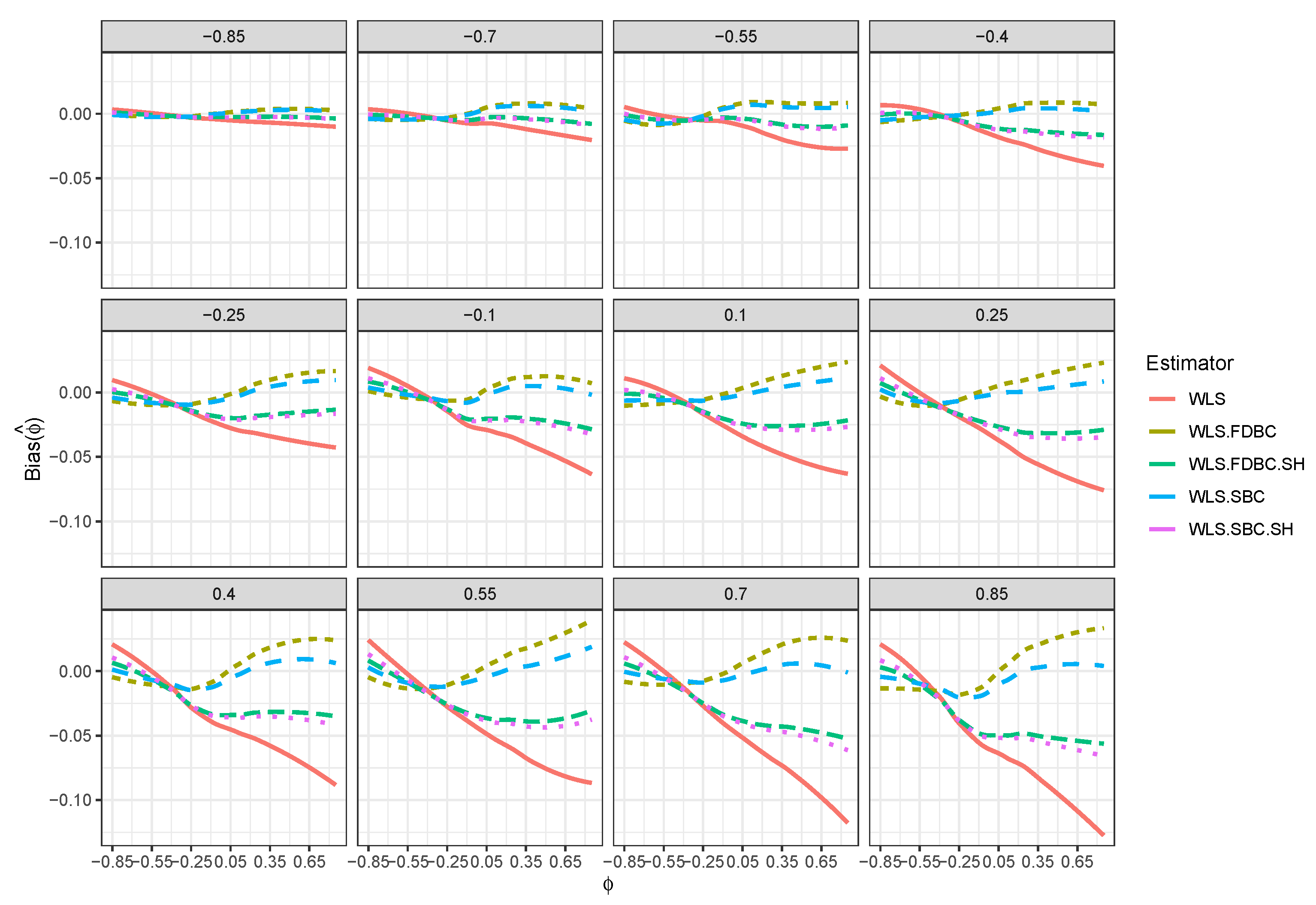
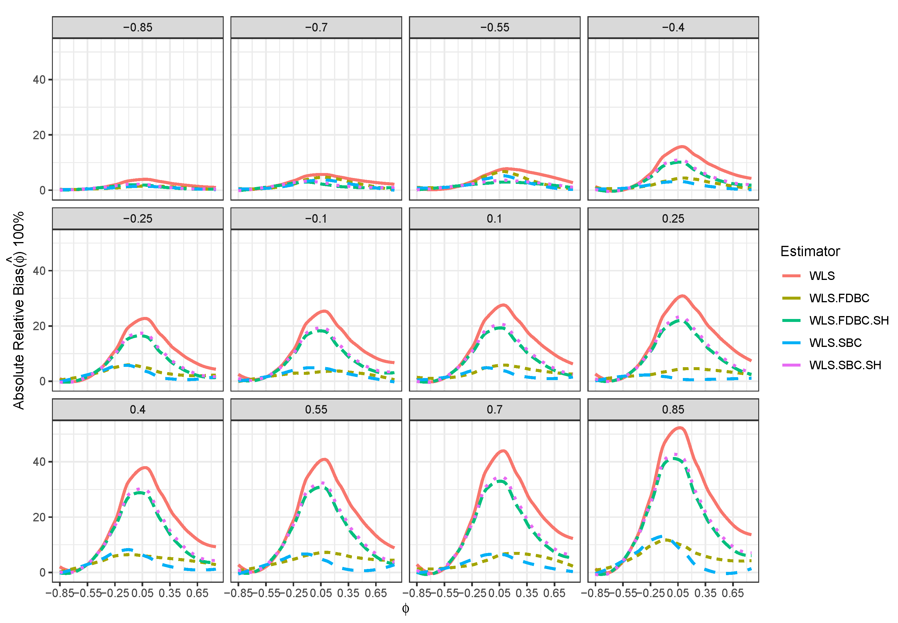
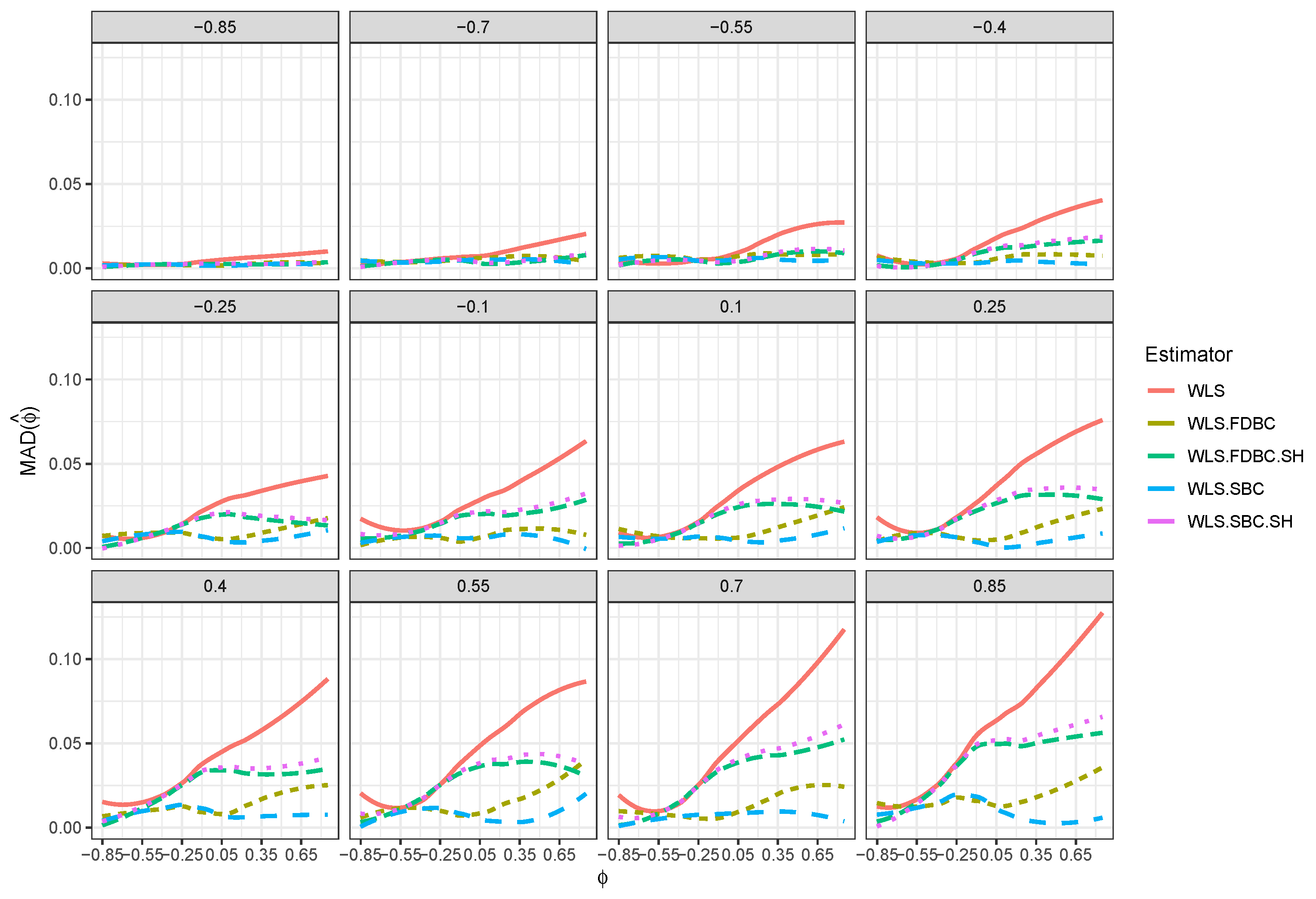
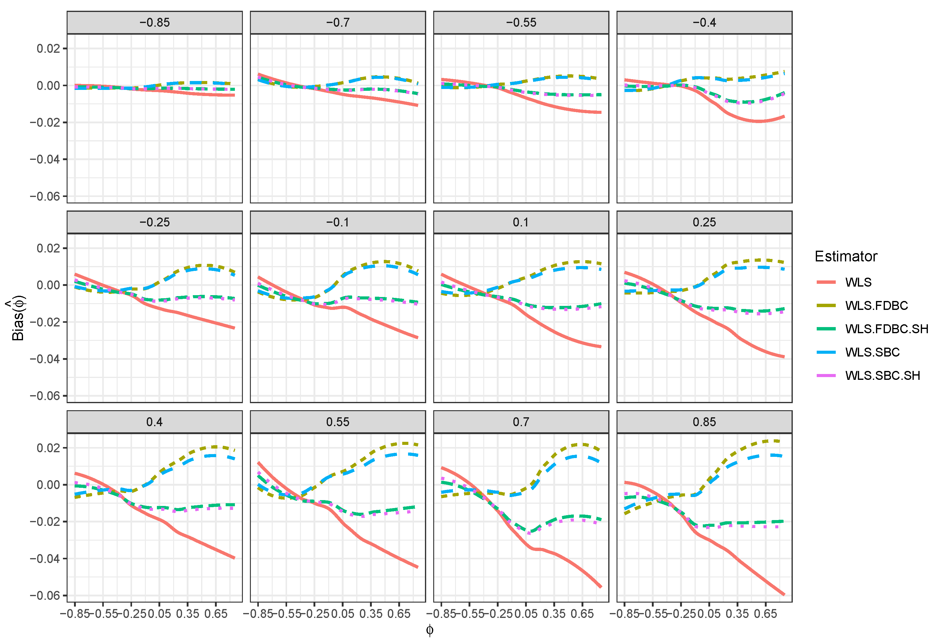
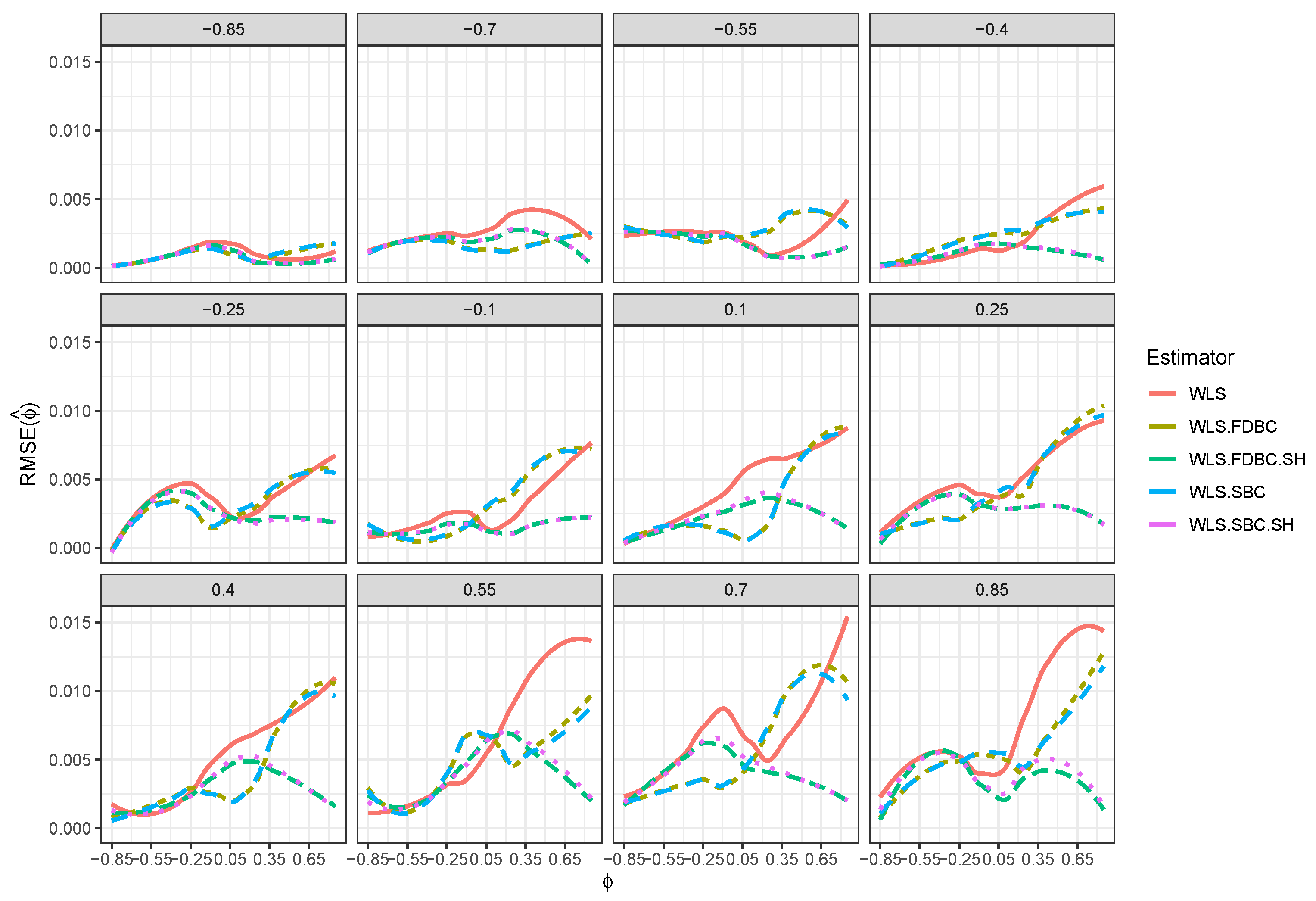
This section provides a summary of the simulation results, as illustrated in Figure 3, Figure 4, Figure 5, Figure 6, Figure 7, Figure 8, Figure 9, Figure 10, Figure 11, Figure 12, Figure 13, Figure 14, Figure 15, Figure 16, Figure 17 and Figure 18. Our examination focuses on four primary metrics: bias, absolute relative bias (ARB), mean absolute deviation (MAD), and root mean squared error (RMSE). These metrics are evaluated across a range of autoregressive coefficients ( ϕ 1 ) and error correlation values ( θ ) for increasing sample sizes. The analysis includes both traditional and shrinkage-based approaches, single bootstrap and fast double bootstrap bias-corrected estimators. The main findings are summarized as follows:
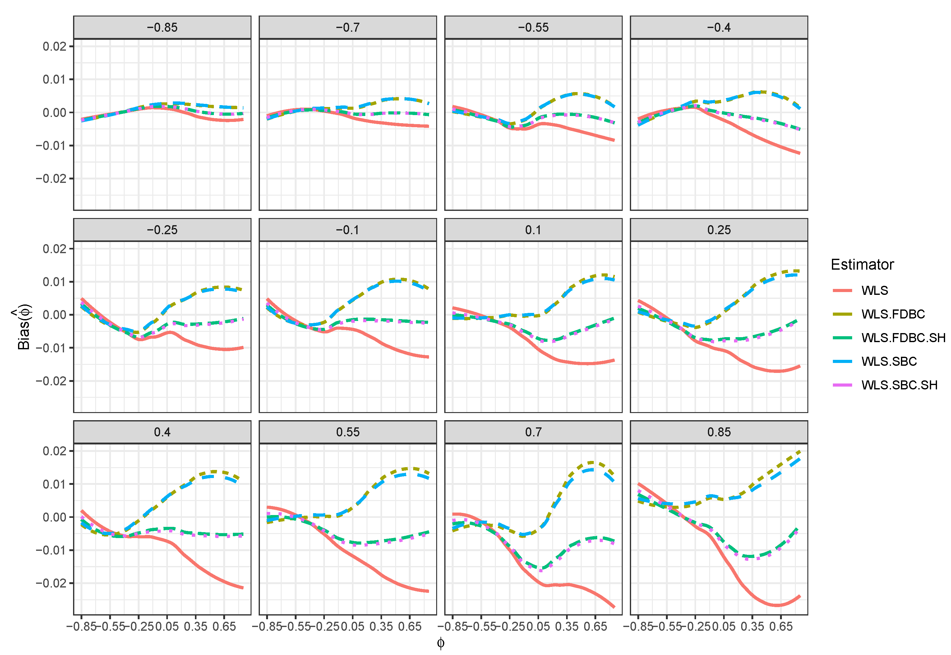
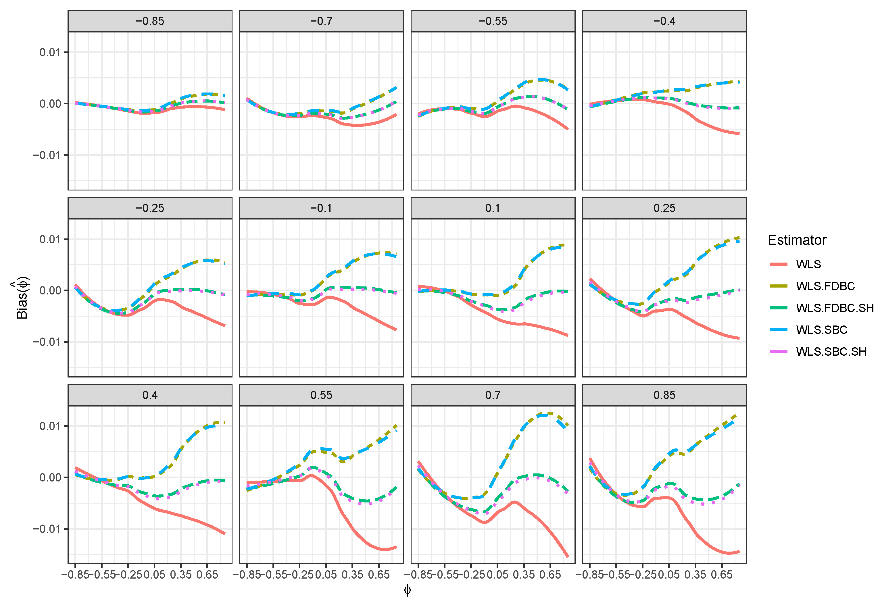
  • In general, the proposed bias-correcting estimators significantly diminished the bias of the WLS estimator across almost all combinations of ϕ 1 and θ . This enhancement is particularly evident in small samples, where the WLS estimator exhibits a consistent and pronounced bias, especially as ϕ 1 shifts from 0.55 to 0.45 depending on the sample size.
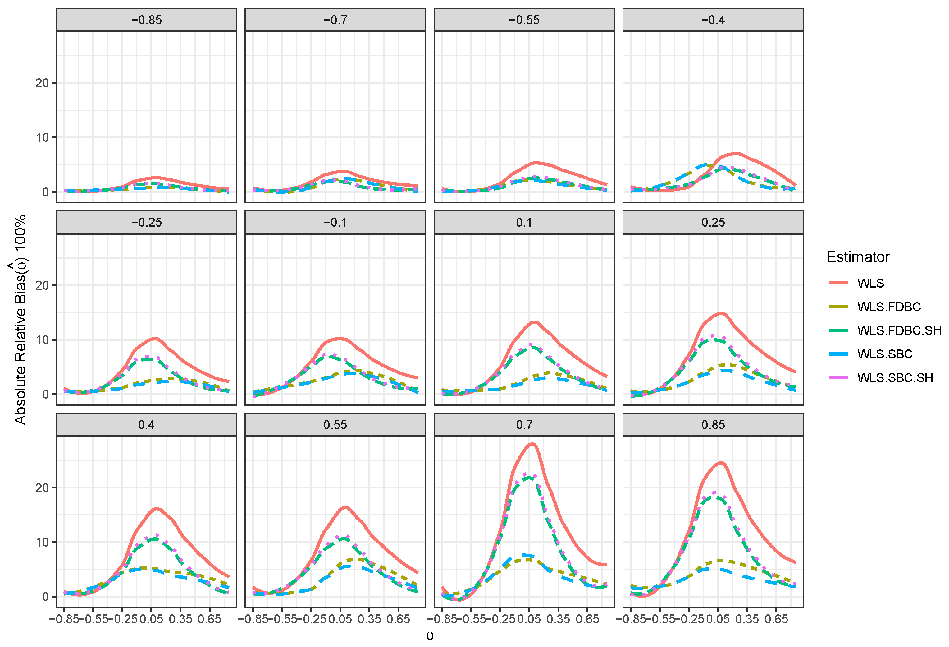
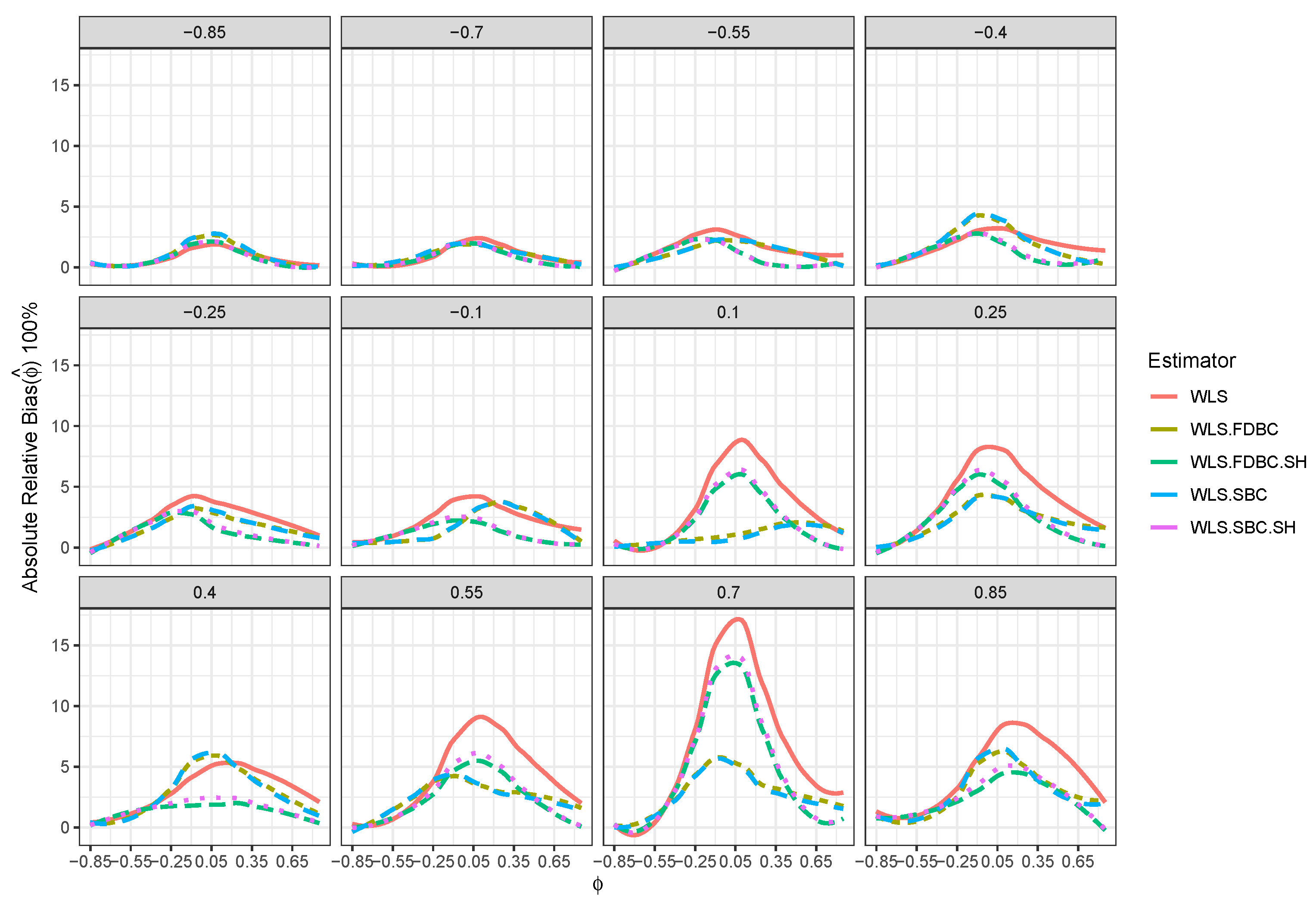
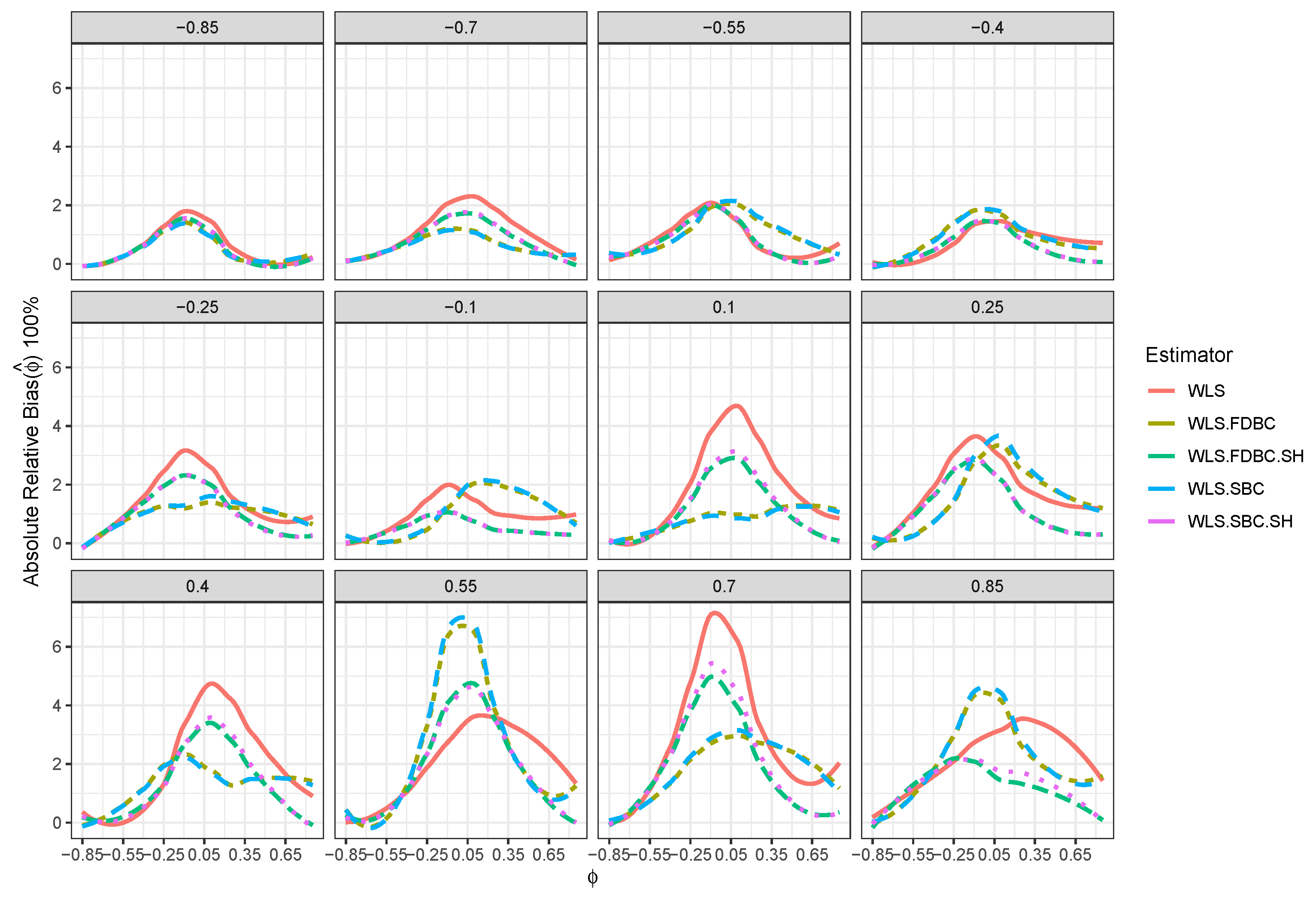
  • Both the traditional single bootstrap ( ϕ ^ 1 SBC ) and fast double bootstrap ( ϕ ^ 1 FDBC ) bias-corrected estimators reduce bias more effectively than the single bootstrap ( ϕ ^ 1 SBC . SH ) and fast double bootstrap ( ϕ ^ 1 FDBC . SH ) bias-corrected estimators based on the shrinking approach. Notably, the single bootstrap estimator outperforms the fast double bootstrap estimator, particularly for small sample sizes (e.g., n = 31 , 63 , 127 ). For example, Figure 4 shows that the single bootstrap bias-corrected estimator reduced the bias by 18 % compared to the WLS estimator for ϕ 1 = 0.85 and θ = 0.25 with n = 31 . Moreover, Figure 8 shows that the traditional single and fast double bootstrap bias-corrected estimators reduced the bias by about 20 % compared to the WLS estimator for ϕ 1 = 0.15 and θ = 0.7 with n = 63 .
  • Despite the bias reduction, some residual bias remains when both θ and ϕ 1 are positive, with the bias increasing as θ and ϕ 1 approach a positive boundary.
  • It is noteworthy that the single bootstrap bias correction often surpasses the fast double bootstrap bias correction in small samples and offers a significantly reduced computational cost, making it a favorable option for practical use.
  • For larger sample sizes, n = 255 , the single bootstrap ( ϕ ^ 1 SBC . SH ) and fast double bootstrap ( ϕ ^ 1 FDBC . SH ) bias-corrected estimators based on the shrinking approach perform better than the traditional single and fast double bootstrap estimators in most of the cases, especially when ϕ 1 0.25 and θ is positive. It is crucial to highlight that traditional bootstrap methods resulted in overcorrection or undercorrection estimators as the sample size increased. The shrinking approach effectively avoids this problem.
  • Although the shrinkage-based bias correction yields noticeable improvements for large sample sizes, some bias remains, particularly when both θ and ϕ 1 are positive. This bias tends to increase as the values of θ and ϕ 1 approach the upper end of their positive boundary.
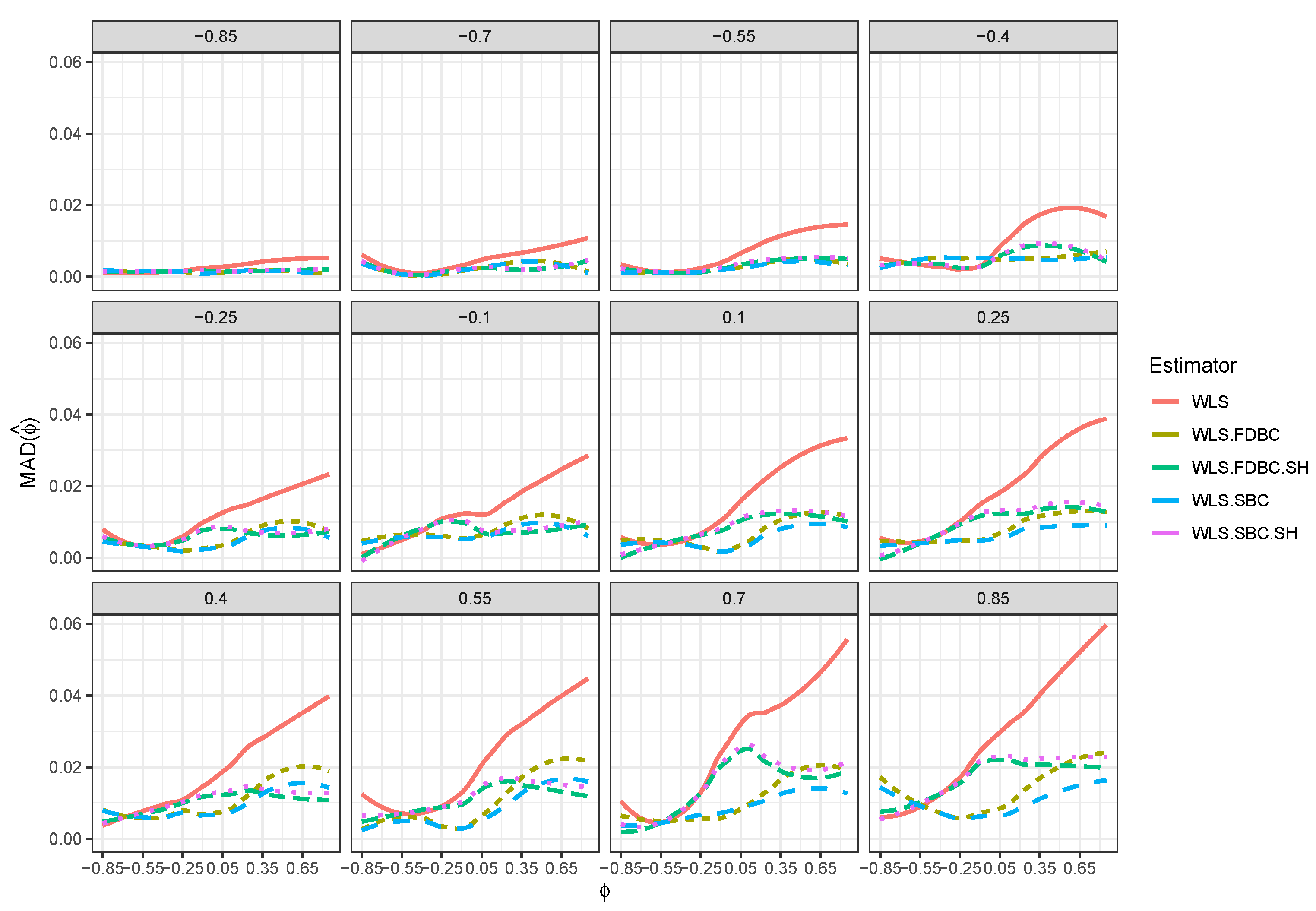
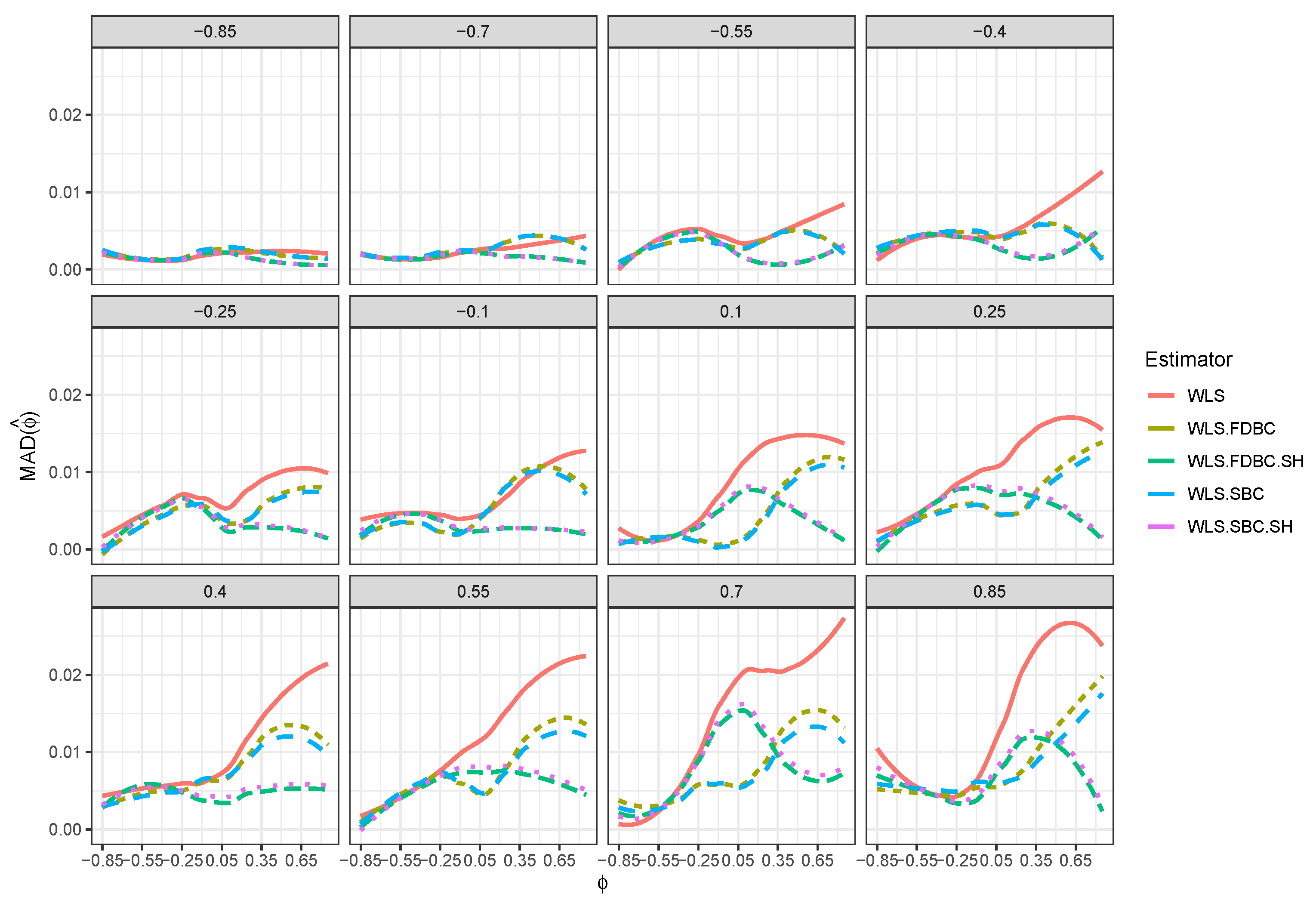
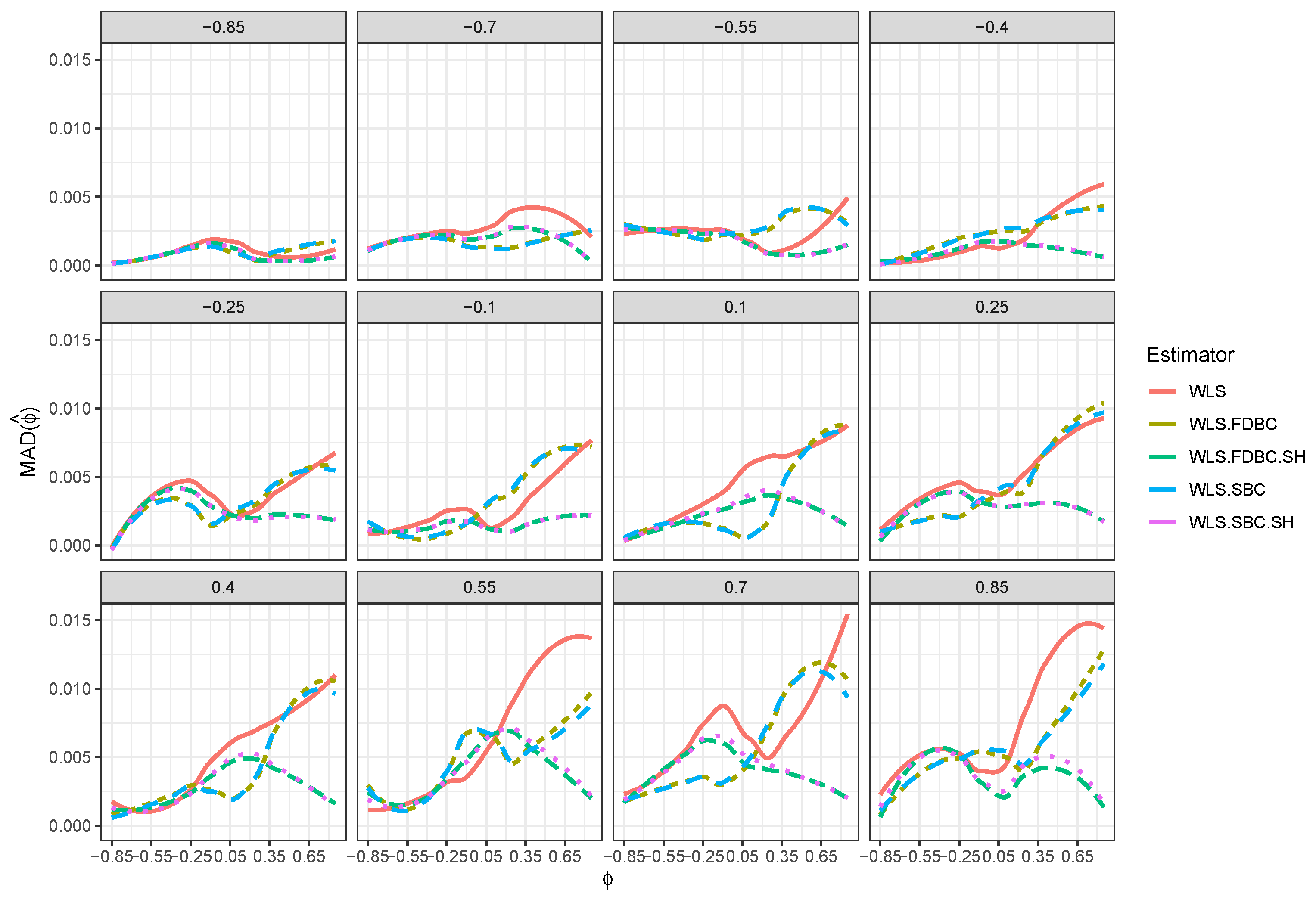
  • All bootstrap methods yielded substantial reductions in both root mean squared error (RMSE) and mean absolute deviation (MAD) relative to the WLS estimator across all sample sizes and for all positive values of θ .
  • Traditional bootstrap bias-correction methods demonstrated notable improvements in RMSE and MAD, particularly for smaller sample sizes (e.g., n = 31 , 63 , 127 ) and positive values of θ , when compared to the uncorrected WLS estimator. For example, Figure 5 and Figure 6 show that when n = 31 , RMSE and MAD improved by about 50% for the single and double bootstrap based on the shrinking approach, compared with the RMSE and MAD of the original WLS estimator ϕ 1 . Moreover, improvements reached nearly 100% for the traditional single and double bootstrap methods in most cases.
  • For larger sample sizes (e.g., n = 255 ), bootstrap bias correction methods based on the shrinkage approach achieved greater reductions in RMSE and MAD than both the WLS estimator and the traditional bootstrap methods, especially across most combinations of ϕ 1 and θ . For example, when θ = 0.85 , the RMSE and MAD for shrinkage-based bootstrap bias correction methods are better than, or at least equivalent to, those of WLS. In contrast, the RMSE and MAD for the traditional single and double bootstrap methods were sometimes higher than those for WLS, particularly when ϕ 1 values are close to zero or greater than 0.25 .
  • Bias reduction to nearly zero from both bootstrap estimators is most evident when ϕ 1 was near the boundaries (i.e., close to 1 or + 1 ), particularly for small sample sizes such as n = 31 . Moreover, the fast double bootstrap method outperformed the single bootstrap approach in reducing bias in the WLS estimators.
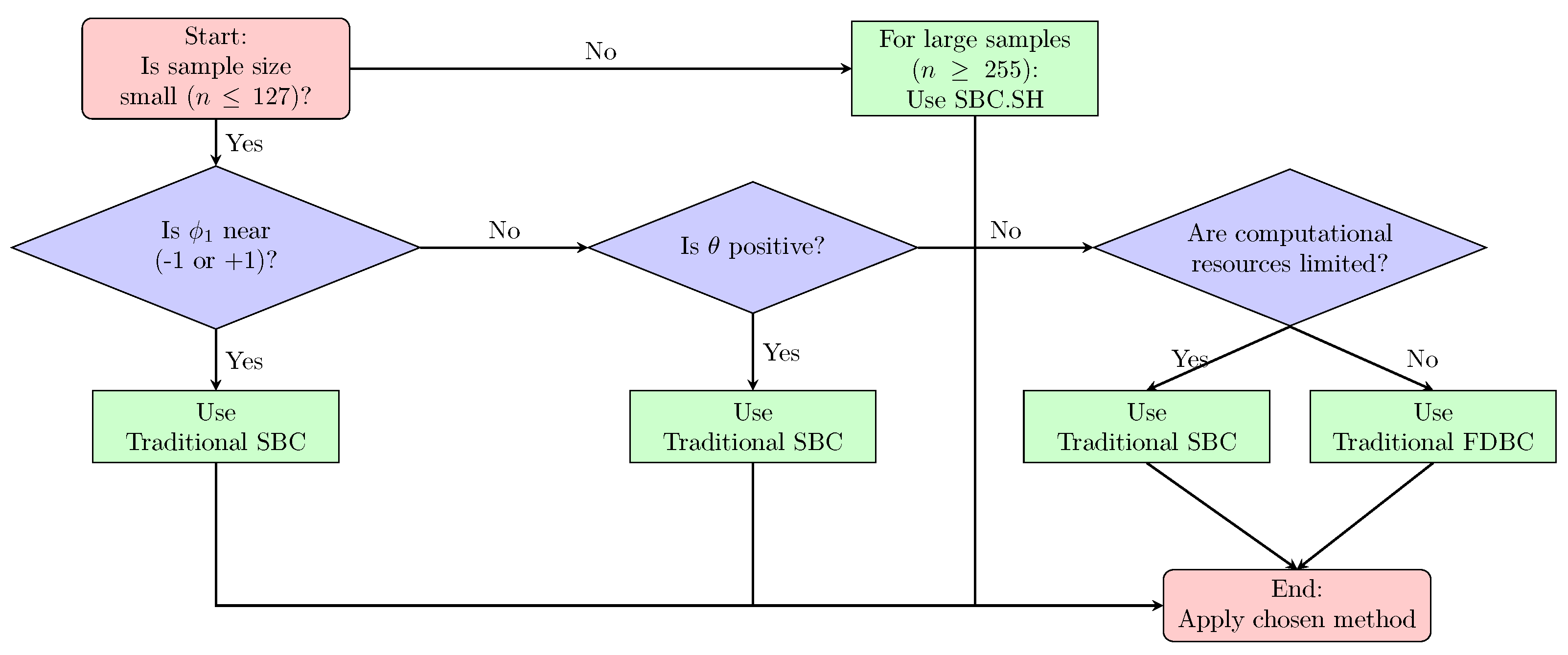
In summary, the results indicate that both the single and fast double bootstrap bias-corrected estimators effectively reduce bias in the WLS estimation of the BAR(1) model across most combinations of ϕ 1 and θ generally, while traditional single and fast double bootstrap techniques perform better in small sample sizes, shrinkage-based bootstrap bias correction methods are more suitable for larger samples. Notably, either the traditional single bootstrap correction or its shrinkage-based counterpart outperforms both the traditional fast double bootstrap and the fast double bootstrap with shrinkage in extreme cases where the autoregressive coefficient approaches its upper boundary. Moreover, the single bootstrap method is less computationally demanding, making it a practical and efficient choice for real-world applications. Based on these findings, we provide clear guidance to practitioners, helping them navigate the choice between different bias correction methods according to their specific circumstances. Figure 19 presents a decision flowchart that guides practitioners in selecting the appropriate bias correction method.

6. Application

This application uses real cell lineage data from [34], specifically tree number 41. Figure 20 illustrates the binary tree, which consists of 31 observations, including two missing values at the first and twenty-first positions (i.e., spanning four generations). The data represent the lifetimes, in minutes, of EMT6 cell lineages.
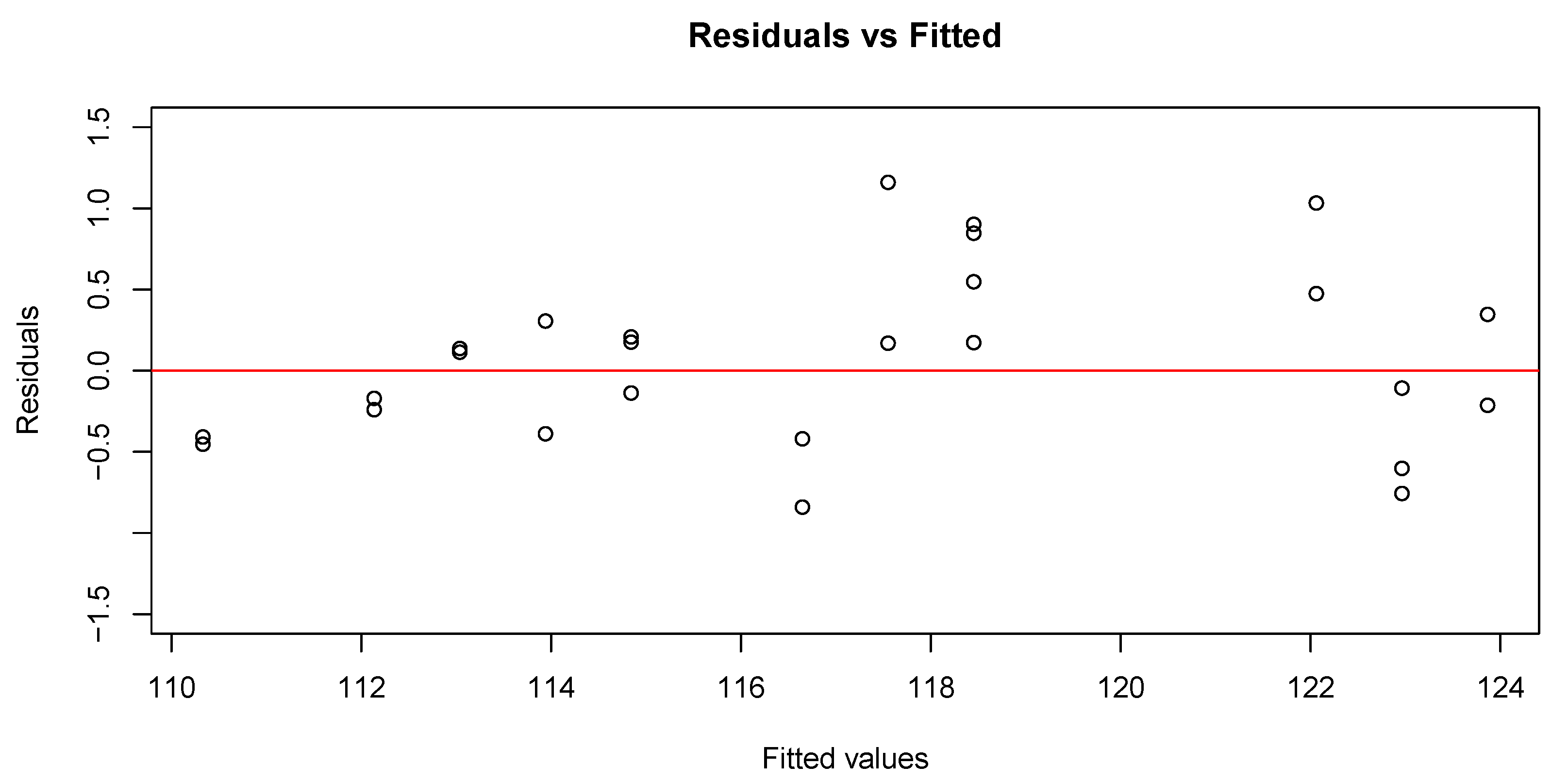
The least squares (LS) estimates of the model parameters are ϕ ^ 1 LS = 0.407 and θ ^ = 0.485 . The residual plot of the LS fit versus the fitted values, shown in Figure 21, indicates non-constant variance, revealing a heteroscedasticity problem in the data.
Using weighted least squares (WLS) estimation, the parameter estimates improve to ϕ ^ 1 WLS = 0.435 and θ ^ = 0.926 . According to the decision flowchart in Figure 19, the sample size is less than 127, the value of ϕ ^ 1 WLS is not close to 1, and θ ^ is positive. Therefore, the appropriate bias correction method is the traditional single bootstrap. Applying this method yields a bias-corrected estimate of the autoregressive coefficient for the BAR(1) model, ϕ ^ 1 WLS . SBC = 0.549 . Looking at Figure 3, in the panel corresponding to θ = 0.85 , the closest available value to θ ^ = 0.926 , and for ϕ 1 0.35 , we observe that the bias of the WLS estimate is under-corrected by about 0.09 . Extrapolating this trend to θ ^ = 0.926 and ϕ 1 = 0.407 , we can infer that the bias is likely larger, falling in the range ( 0.15 , 0.10 ) . Comparing this to the bias-corrected estimate ϕ ^ 1 WLS . SBC = 0.549 , we find that the corrected estimate falls within the interval ( 0.535 , 0.585 ) . This outcome validates both our simulation findings and the decision workflow strategy.

7. Conclusions and Discussion

This study evaluated the bias in the weighted least squares (WLS) estimator in first-order bifurcating autoregressive (BAR(1)) models when the sample size is small or moderate. The WLS estimator is well-known in statistical literature for its ability to handle varying error variances. However, it can be biased with small or moderate samples. For the autoregressive coefficient of the BAR(1) model, the size and direction of this bias depend on the autoregressive parameter ( ϕ 1 ) and the correlation among the error terms ( θ ). To address this issue, four bias-corrected methods for the WLS estimator based on bootstrap techniques are suggested. This study explored the traditional bias correction using a single bootstrap, fast double bootstrap approaches, and related shrinkage approaches to prevent the under- or over-correction that may occur. The simulation results indicate that the proposed corrections significantly decrease the bias in the WLS estimates. This reduction is associated with improvements in the root mean square error (RMSE), showing better efficiency. The traditional single bootstrap correction performed best for small and moderate sample sizes, while the shrinkage-based single bootstrap yielded the best results for larger samples.
The limitations of the proposed bias-correction methods need further discussion. Bootstrap bias corrections are based on models and require correctly specifying the BAR(1) process, which assumes a stationary process that may not fit some real data. Additionally, deviations from this assumption, like higher-order BAR structures or non-stationary processes, could challenge the validity of the corrections. Furthermore, improper specification of the correlation structure for the error terms may lead to unreliable coefficient estimates. The simulation study relied on the assumption of a bivariate normal error distribution. However, in practice, issues like skewness or heavy tails can arise. In these cases, the authors point to [17,35], which explore these issues in depth. Additionally, while the analysis included heteroscedasticity in the form of increasing error variance, more complex variance structures could arise in future studies. Addressing these situations may require bias correction methods that extend beyond the current approach.
From a computational perspective, bias correction methods that rely on the bootstrap technique, particularly the fast double bootstrap, are resource-intensive for large samples. This limitation might restrict their use on personal computers, highlighting the need for more efficient implementations, such as using high-performance computing. Finally, the results suggest that the corrected autoregressive estimates for the BAR(1) model may be under- or over-corrected, especially as the sample size increases. This finding stresses the importance of careful application and encourages the development of adaptive strategies to mitigate such risks.
In conclusion, the findings reveal that bootstrap-based bias correction methods can substantially improve the performance of WLS estimators in BAR(1) models. It is essential to address the identified limitations to enhance the reliability and practical effectiveness of these methods, thereby advancing statistical modeling in studies of cell lineage and related branching processes.

Author Contributions

Conceptualization, methodology, T.E., S.M. and A.A.; software, formal analysis and investigation, writing—original draft preparation, T.E.; writing—review and editing, T.E., M.U., S.M., M.Z. and A.A. All authors have read and agreed to the published version of the manuscript.

Funding

This research received no external funding.

Data Availability Statement

Codes supporting this study’s findings may be obtained from the corresponding author upon request.

Conflicts of Interest

The authors declare no conflicts of interest.

References

  1. Cowan, R. Statistical Concepts in the Analysis of Cell Lineage Data. In Proceedings of the 1983 Workshop Cell Growth Division; Latrobe University: Melbourne, Australia, 1984; pp. 18–22. [Google Scholar]
  2. Hawkins, E.D.; Markham, J.F.; McGuinness, L.P.; Hodgkin, P.D. A single-cell pedigree analysis of alternative stochastic lymphocyte fates. Proc. Natl. Acad. Sci. USA 2009, 106, 13457–13462. [Google Scholar] [CrossRef] [PubMed]
  3. Kimmel, M.; Axelrod, D. Branching Processes in Biology; Springer: New York, NY, USA, 2005. [Google Scholar]
  4. Sandler, O.; Mizrahi, S.P.; Weiss, N.; Agam, O.; Simon, I.; Balaban, N.Q. Lineage correlations of single cell division time as a probe of cell-cycle dynamics. Nature 2015, 519, 468–471. [Google Scholar] [CrossRef] [PubMed]
  5. Cowan, R.; Staudte, R. The Bifurcating Autoregression Model in Cell Lineage Studies. Biometrics 1986, 42, 769–783. [Google Scholar] [CrossRef] [PubMed]
  6. Huggins, R.M. A law of large numbers for the bifurcating autoregressive process. Commun. Stat. Stoch. Model. 1995, 11, 273–278. [Google Scholar] [CrossRef]
  7. Bui, Q.; Huggins, R. Inference for the random coefficients bifurcating autoregressive model for cell lineage studies. J. Stat. Plan. Inference 1999, 81, 253–262. [Google Scholar] [CrossRef]
  8. Huggins, R.M.; Basawa, I.V. Extensions of the Bifurcating Autoregressive Model for Cell Lineage Studies. J. Appl. Probab. 1999, 36, 1225–1233. [Google Scholar] [CrossRef]
  9. Huggins, R.; Basawa, I. Inference for the extended bifurcating autoregressive model for cell lineage studies. Aust. N. Z. J. Stat. 2000, 42, 423–432. [Google Scholar] [CrossRef]
  10. Zhou, J.; Basawa, I. Least-squares estimation for bifurcating autoregressive processes. Stat. Probab. Lett. 2005, 74, 77–88. [Google Scholar] [CrossRef]
  11. Terpstra, J.T.; Elbayoumi, T. A law of large numbers result for a bifurcating process with an infinite moving average representation. Stat. Probab. Lett. 2012, 82, 123–129. [Google Scholar] [CrossRef]
  12. Elbayoumi, T.; Terpstra, J. Weighted L1-Estimates for the First-order Bifurcating Autoregressive Model. Commun. Stat. Simul. Comput. 2016, 45, 2991–3013. [Google Scholar] [CrossRef]
  13. Elbayoumi, T.M.; Mostafa, S.A. On the estimation bias in first-order bifurcating autoregressive models. Stat 2021, 10, e342. [Google Scholar] [CrossRef]
  14. Hurwicz, L. Least-squares bias in time series. In Statistical Inference in Dynamic Economic Models; John Wiley & Sons, Inc.: Hoboken, NJ, USA, 1950; pp. 365–383. [Google Scholar]
  15. Huggins, R.M.; Marschner, I.C. Robust Analysis of the Bifurcating Autoregressive Model in Cell Lineage Studies. Aust. N. Z. J. Stat. 1991, 33, 209–220. [Google Scholar] [CrossRef]
  16. Staudte, R.G. A bifurcating autoregression model for cell lineages with variable generation means. J. Theor. Biol. 1992, 156, 183–195. [Google Scholar] [CrossRef]
  17. Elbayoumi, T.; Mostafa, S. Bias Analysis and Correction in Weighted-L1 Estimators for the First-Order Bifurcating Autoregressive Model. Stats 2024, 7, 1315–1332. [Google Scholar] [CrossRef]
  18. Blandin, V. Asymptotic results for random coefficient bifurcating autoregressive processes. Statistics 2014, 48, 1202–1232. [Google Scholar] [CrossRef]
  19. MacKinnon, J.G.; Smith, A.A. Approximate bias correction in econometrics. J. Econom. 1998, 85, 205–230. [Google Scholar] [CrossRef]
  20. Berkowitz, J.; Kilian, L. Recent developments in bootstrapping time series. Econom. Rev. 2000, 19, 1–48. [Google Scholar] [CrossRef]
  21. Tanizaki, H.; Hamori, S.; Matsubayashi, Y. On least-squares bias in the AR(p) models: Bias correction using the bootstrap methods. Stat. Pap. 2006, 47, 109–124. [Google Scholar] [CrossRef]
  22. Patterson, K. Bias Reduction through First-order Mean Correction, Bootstrapping and Recursive Mean Adjustment. J. Appl. Stat. 2007, 34, 23–45. [Google Scholar] [CrossRef]
  23. Liu-Evans, G.D.; Phillips, G.D. Bootstrap, Jackknife and COLS: Bias and Mean Squared Error in Estimation of Autoregressive Models. J. Time Ser. Econom. 2012, 4, 1–33. [Google Scholar] [CrossRef]
  24. Hall, P. The Bootstrap and Edgeworth Expansion; Springer: New York, NY, USA, 1992. [Google Scholar]
  25. Lee, S.M.S.; Young, G.A. The effect of Monte Carlo approximation on coverage error of double-bootstrap confidence intervals. J. R. Stat. Soc. Ser. 1999, 61, 353–366. [Google Scholar] [CrossRef]
  26. Shi, S.G. Accurate and Efficient Double-bootstrap Confidence Limit Method. Comput. Stat. Data Anal. 1992, 13, 21–32. [Google Scholar] [CrossRef]
  27. Chang, J.; Hall, P. Double-bootstrap methods that use a single double-bootstrap simulation. Biometrika 2015, 102, 203–214. [Google Scholar] [CrossRef]
  28. Ouysse, R. A Fast Iterated Bootstrap Procedure for Approximating the Small-Sample Bias. Commun. Stat. Simul. Comput. 2013, 42, 1472–1494. [Google Scholar] [CrossRef]
  29. Tibbe, T.D.; Montoya, A.K. Correcting the Bias Correction for the Bootstrap Confidence Interval in Mediation Analysis. Front. Psychol. 2022, 13, 810258. [Google Scholar] [CrossRef]
  30. Song, E.; Lam, H.; Barton, R.R. A Shrinkage Approach to Improve Direct Bootstrap Resampling Under Input Uncertainty. INFORMS J. Comput. 2024, 36, 1023–1039. [Google Scholar] [CrossRef]
  31. Tibshirani, R. Regression Shrinkage and Selection via the Lasso. J. R. Stat. Soc. Ser. 1996, 58, 267–288. [Google Scholar] [CrossRef]
  32. R Core Team. R: A Language and Environment for Statistical Computing; R Foundation for Statistical Computing: Vienna, Austria, 2022. [Google Scholar]
  33. Elbayoumi, T.; Mostafa, S. Bifurcatingr: Bifurcating Autoregressive Models, R package version 2.1.0; R Foundation for Statistical Computing: Vienna, Austria, 2024; Available online: https://CRAN.R-project.org/package=bifurcatingr (accessed on 25 August 2025).
  34. Huggins, R.M. Robust Inference for Variance Components Models for Single Trees of Cell Lineage Data. Ann. Stat. 1996, 24, 1145–1160. Available online: http://www.jstor.org/stable/2242586 (accessed on 25 August 2025). [CrossRef]
  35. Elbayoumi, T.; Mostafa, S. Impact of Bias Correction of the Least Squares Estimation on Bootstrap Confidence Intervals for Bifurcating Autoregressive Models. J. Data Sci. 2024, 22, 25–44. [Google Scholar] [CrossRef]
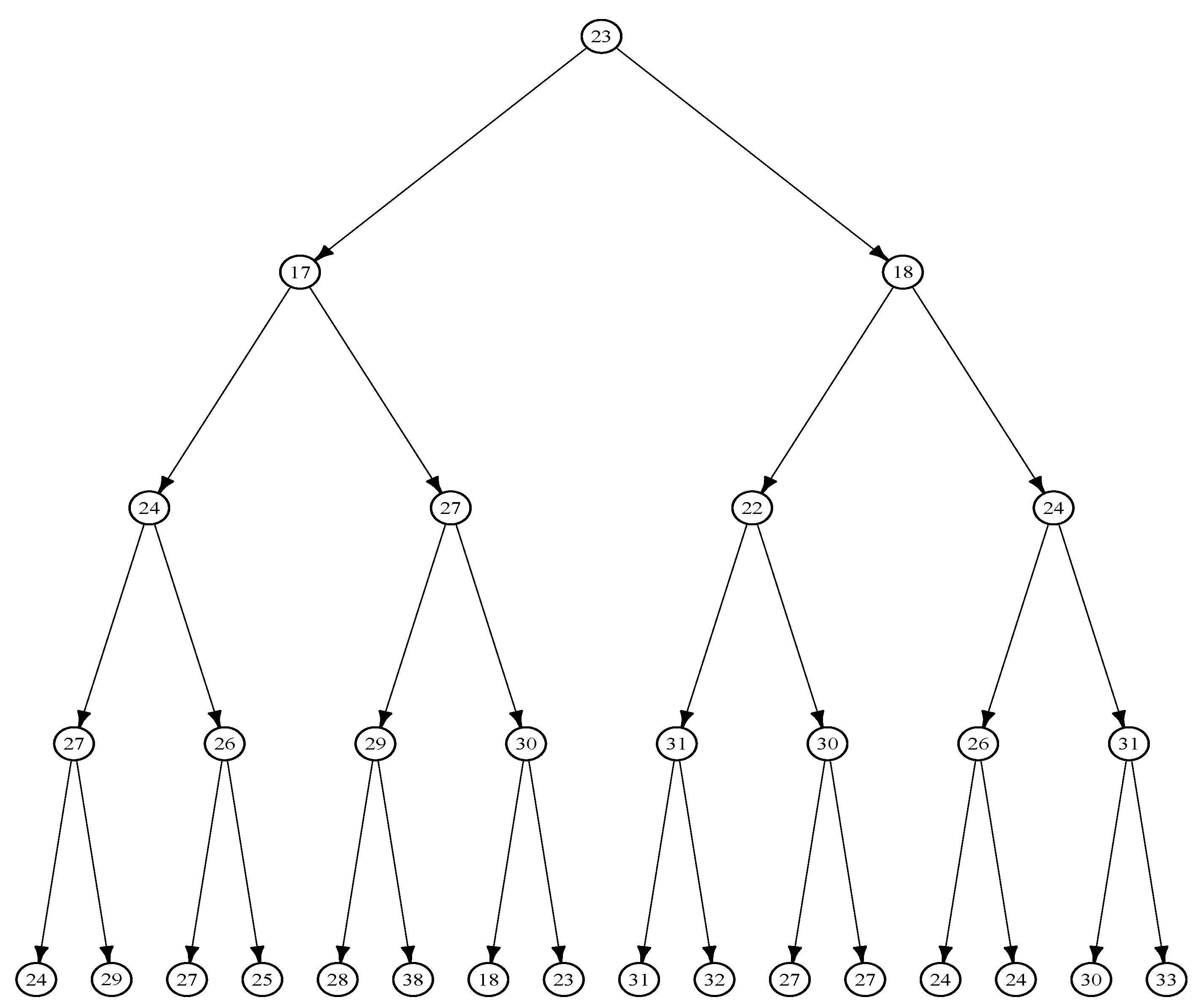
Figure 1. The tree displays E. coli cell lifetimes (in minutes), derived from the data in [5].
Stats 08 00079 g001
Figure 2. Empirical bias, ARB (%), variance, and MSE of the WLS estimator of ϕ 1 when the error distribution is bivariate normal with mean zero and a heteroscedastic variance-covariance structure increase with time according to σ t = σ t .
Stats 08 00079 g002
Figure 3. The bias of the WLS estimator ( ϕ ^ 1 WLS ), traditional single bootstrap bias-corrected estimator ( ϕ ^ 1 WLS . SBC ), traditional fast double bootstrap bias-corrected estimator ( ϕ ^ 1 WLS . FDBC ), single bootstrap bias-corrected estimator based on the shrinking approach ( ϕ ^ 1 WLS . SBC . SH ), and fast double bootstrap bias-corrected estimator based on the shrinking approach ( ϕ ^ 1 WLS . FDBC . SH ) estimators as a function of ϕ 1 at different levels of θ with a sample size n = 31 .
Stats 08 00079 g003
Figure 4. The ARB of the WLS estimator ( ϕ ^ 1 WLS ), traditional single bootstrap bias-corrected estimator ( ϕ ^ 1 WLS . SBC ), traditional fast double bootstrap bias-corrected estimator ( ϕ ^ 1 WLS . FDBC ), single bootstrap bias-corrected estimator based on the shrinking approach ( ϕ ^ 1 WLS . SBC . SH ), and fast double bootstrap bias-corrected estimator based on the shrinking approach ( ϕ ^ 1 WLS . FDBC . SH ) estimators as a function of ϕ 1 at different levels of θ with a sample size n = 31 .
Stats 08 00079 g004
Figure 5. The MAD of the WLS estimator ( ϕ ^ 1 WLS ), traditional single bootstrap bias-corrected estimator ( ϕ ^ 1 WLS . SBC ), traditional fast double bootstrap bias-corrected estimator ( ϕ ^ 1 WLS . FDBC ), single bootstrap bias-corrected estimator based on the shrinking approach ( ϕ ^ 1 WLS . SBC . SH ), and fast double bootstrap bias-corrected estimator based on the shrinking approach ( ϕ ^ 1 WLS . FDBC . SH ) estimators as a function of ϕ 1 at different levels of θ with a sample size n = 31 .
Stats 08 00079 g005
Figure 6. The RMSE of the WLS estimator ( ϕ ^ 1 WLS ), traditional single bootstrap bias-corrected estimator ( ϕ ^ 1 WLS . SBC ), traditional fast double bootstrap bias-corrected estimator ( ϕ ^ 1 WLS . FDBC ), single bootstrap bias-corrected estimator based on the shrinking approach ( ϕ ^ 1 WLS . SBC . SH ), and fast double bootstrap bias-corrected estimator based on the shrinking approach ( ϕ ^ 1 WLS . FDBC . SH ) estimators as a function of ϕ 1 at different levels of θ with a sample size n = 31 .
Stats 08 00079 g006
Figure 7. The bias of the WLS estimator ( ϕ ^ 1 WLS ), traditional single bootstrap bias-corrected estimator ( ϕ ^ 1 WLS . SBC ), traditional fast double bootstrap bias-corrected estimator ( ϕ ^ 1 WLS . FDBC ), single bootstrap bias-corrected estimator based on the shrinking approach ( ϕ ^ 1 WLS . SBC . SH ), and fast double bootstrap bias-corrected estimator based on the shrinking approach ( ϕ ^ 1 WLS . FDBC . SH ) estimators as a function of ϕ 1 at different levels of θ with a sample size n = 63 .
Stats 08 00079 g007
Figure 8. The ARB of the WLS estimator ( ϕ ^ 1 WLS ), traditional single bootstrap bias-corrected estimator ( ϕ ^ 1 WLS . SBC ), traditional fast double bootstrap bias-corrected estimator ( ϕ ^ 1 WLS . FDBC ), single bootstrap bias-corrected estimator based on the shrinking approach ( ϕ ^ 1 WLS . SBC . SH ), and fast double bootstrap bias-corrected estimator based on the shrinking approach ( ϕ ^ 1 WLS . FDBC . SH ) estimators as a function of ϕ 1 at different levels of θ with a sample size n = 63 .
Stats 08 00079 g008
Figure 9. The MAD of the WLS estimator ( ϕ ^ 1 WLS ), traditional single bootstrap bias-corrected estimator ( ϕ ^ 1 WLS . SBC ), traditional fast double bootstrap bias-corrected estimator ( ϕ ^ 1 WLS . FDBC ), single bootstrap bias-corrected estimator based on the shrinking approach ( ϕ ^ 1 WLS . SBC . SH ), and fast double bootstrap bias-corrected estimator based on the shrinking approach ( ϕ ^ 1 WLS . FDBC . SH ) estimators as a function of ϕ 1 at different levels of θ with a sample size n = 63 .
Stats 08 00079 g009
Figure 10. The RMSE of the WLS estimator ( ϕ ^ 1 WLS ), traditional single bootstrap bias-corrected estimator ( ϕ ^ 1 WLS . SBC ), traditional fast double bootstrap bias-corrected estimator ( ϕ ^ 1 WLS . FDBC ), single bootstrap bias-corrected estimator based on the shrinking approach ( ϕ ^ 1 WLS . SBC . SH ), and fast double bootstrap bias-corrected estimator based on the shrinking approach ( ϕ ^ 1 WLS . FDBC . SH ) estimators as a function of ϕ 1 at different levels of θ with a sample size n = 63 .
Stats 08 00079 g010
Figure 11. The bias of the WLS estimator ( ϕ ^ 1 WLS ), traditional single bootstrap bias-corrected estimator ( ϕ ^ 1 WLS . SBC ), traditional fast double bootstrap bias-corrected estimator ( ϕ ^ 1 WLS . FDBC ), single bootstrap bias-corrected estimator based on the shrinking approach ( ϕ ^ 1 WLS . SBC . SH ), and fast double bootstrap bias-corrected estimator based on the shrinking approach ( ϕ ^ 1 WLS . FDBC . SH ) estimators as a function of ϕ 1 at different levels of θ with a sample size n = 127 .
Stats 08 00079 g011
Figure 12. The ARB of the WLS estimator ( ϕ ^ 1 WLS ), traditional single bootstrap bias-corrected estimator ( ϕ ^ 1 WLS . SBC ), traditional fast double bootstrap bias-corrected estimator ( ϕ ^ 1 WLS . FDBC ), single bootstrap bias-corrected estimator based on the shrinking approach ( ϕ ^ 1 WLS . SBC . SH ), and fast double bootstrap bias-corrected estimator based on the shrinking approach ( ϕ ^ 1 WLS . FDBC . SH ) estimators as a function of ϕ 1 at different levels of θ with a sample size n = 127 .
Stats 08 00079 g012
Figure 13. The MAD of the WLS estimator ( ϕ ^ 1 WLS ), traditional single bootstrap bias-corrected estimator ( ϕ ^ 1 WLS . SBC ), traditional fast double bootstrap bias-corrected estimator ( ϕ ^ 1 WLS . FDBC ), single bootstrap bias-corrected estimator based on the shrinking approach ( ϕ ^ 1 WLS . SBC . SH ), and fast double bootstrap bias-corrected estimator based on the shrinking approach ( ϕ ^ 1 WLS . FDBC . SH ) estimators as a function of ϕ 1 at different levels of θ with a sample size n = 127 .
Stats 08 00079 g013
Figure 14. The RMSE of the WLS estimator ( ϕ ^ 1 WLS ), traditional single bootstrap bias-corrected estimator ( ϕ ^ 1 WLS . SBC ), traditional fast double bootstrap bias-corrected estimator ( ϕ ^ 1 WLS . FDBC ), single bootstrap bias-corrected estimator based on the shrinking approach ( ϕ ^ 1 WLS . SBC . SH ), and fast double bootstrap bias-corrected estimator based on the shrinking approach ( ϕ ^ 1 WLS . FDBC . SH ) estimators as a function of ϕ 1 at different levels of θ with a sample size n = 127 .
Stats 08 00079 g014
Figure 15. The bias of the WLS estimator ( ϕ ^ 1 WLS ), traditional single bootstrap bias-corrected estimator ( ϕ ^ 1 WLS . SBC ), traditional fast double bootstrap bias-corrected estimator ( ϕ ^ 1 WLS . FDBC ), single bootstrap bias-corrected estimator based on the shrinking approach ( ϕ ^ 1 WLS . SBC . SH ), and fast double bootstrap bias-corrected estimator based on the shrinking approach ( ϕ ^ 1 WLS . FDBC . SH ) estimators as a function of ϕ 1 at different levels of θ with a sample size n = 255 .
Stats 08 00079 g015
Figure 16. The ARB of the WLS estimator ( ϕ ^ 1 WLS ), traditional single bootstrap bias-corrected estimator ( ϕ ^ 1 WLS . SBC ), traditional fast double bootstrap bias-corrected estimator ( ϕ ^ 1 WLS . FDBC ), single bootstrap bias-corrected estimator based on the shrinking approach ( ϕ ^ 1 WLS . SBC . SH ), and fast double bootstrap bias-corrected estimator based on the shrinking approach ( ϕ ^ 1 WLS . FDBC . SH ) estimators as a function of ϕ 1 at different levels of θ with a sample size n = 255 .
Stats 08 00079 g016
Figure 17. The MAD of the WLS estimator ( ϕ ^ 1 WLS ), traditional single bootstrap bias-corrected estimator ( ϕ ^ 1 WLS . SBC ), traditional fast double bootstrap bias-corrected estimator ( ϕ ^ 1 WLS . FDBC ), single bootstrap bias-corrected estimator based on the shrinking approach ( ϕ ^ 1 WLS . SBC . SH ), and fast double bootstrap bias-corrected estimator based on the shrinking approach ( ϕ ^ 1 WLS . FDBC . SH ) estimators as a function of ϕ 1 at different levels of θ with a sample size n = 255 .
Stats 08 00079 g017
Figure 18. The RMSE of the WLS estimator ( ϕ ^ 1 WLS ), traditional single bootstrap bias-corrected estimator ( ϕ ^ 1 WLS . SBC ), traditional fast double bootstrap bias-corrected estimator ( ϕ ^ 1 WLS . FDBC ), single bootstrap bias-corrected estimator based on the shrinking approach ( ϕ ^ 1 WLS . SBC . SH ), and fast double bootstrap bias-corrected estimator based on the shrinking approach ( ϕ ^ 1 WLS . FDBC . SH ) estimators as a function of ϕ 1 at different levels of θ with a sample size n = 255 .
Stats 08 00079 g018
Figure 19. Decision flowchart for selecting a bias correction method for weighted least squares (WLS) estimators of the bifurcating autoregressive parameter, ϕ 1 , in the BAR(1) model.
Stats 08 00079 g019
Figure 20. Binary lineage tree of EMT6 cells, corresponding to Tree 41 in [34].
Stats 08 00079 g020
Figure 21. Diagnostic plot of residuals versus fitted values for the BAR(1) model obtained via least squares estimation.
Stats 08 00079 g021
Table 1. Summary of Simulation Scenarios.
ParameterValues
Sample size (n)31, 63, 127, 255
Autoregressive coefficient (ϕ1)±0.10, ±0.25, ±0.55, ±0.85
Error correlation (θ)±0.10, ±0.25, ±0.55, ±0.85
Intercept (ϕ0)10 (fixed)
Error distributionBivariate normal with mean zero
Variance structureHeteroscedastic: σ t = σ t
Number of Monte Carlo replications10,000
Disclaimer/Publisher’s Note: The statements, opinions and data contained in all publications are solely those of the individual author(s) and contributor(s) and not of MDPI and/or the editor(s). MDPI and/or the editor(s) disclaim responsibility for any injury to people or property resulting from any ideas, methods, instructions or products referred to in the content.