A Bayesian Non-Linear Mixed-Effects Model for Accurate Detection of the Onset of Cognitive Decline in Longitudinal Aging Studies

Abstract

Change-point models are frequently considered when modeling phenomena where a regime shift occurs at an unknown time. In aging research, these models are commonly adopted to estimate of the onset of cognitive decline. Yet these models present several limitations. Here, we present a Bayesian non-linear mixed-effects model based on a differential equation designed for longitudinal studies to overcome some limitations of classical change point models used in aging research. We demonstrate the ability of the proposed model to avoid biases in estimates of the onset of cognitive impairment in a simulated study. Finally, the methodology presented in this work is illustrated by analyzing results from memory tests from older adults who participated in the English Longitudinal Study of Aging.

1. Introduction

In aging research, determining the onset of cognitive decline is highly relevant, since its accurate and early detection allows for a better understanding of the aging process, its characteristics, and factors associated with its onset [1]. Early detection is therefore critical for the implementation of preventive or therapeutic interventions that can slow or mitigate cognitive decline. The inaccurate estimation of this onset can have significant and potentially harmful consequences; for instance, overestimation of cognitive decline onset may result in delayed care provision for older adults. On the other hand, underestimating the onset of cognitive decline can lead to unnecessary anxiety and worry. Caregivers may think that older persons are in a more advanced state of cognitive deterioration than they are, negatively impacting their quality of life and emotional well-being. Therefore, there is a need for methods that permit the accurate estimation of the onset of cognitive decline in older adults, backed by solid data and appropriate clinical assessments.

Change-point (CP) models are commonly used in aging research for estimating the onset of cognitive decline [2,3,4] and answering questions concerned with the timing of processes such as terminal decline [5]. The detection of the moment at which a CP occurs in the trajectory of a stochastic process is a problem that has been addressed from multiple perspectives in different disciplines. It is a common problem in time series analysis [6] and of utmost interest in longitudinal studies, where a set of individuals is followed over time. Although both types of studies aim to obtain predictions about the behavior of paths of stochastic processes, longitudinal studies usually pay more attention to the determinants of the phenomenon under investigation. In this sense, statistical analysis is frequently performed in the context of regression models, often including random effects. Change-point regression models are commonly formulated in longitudinal studies within a framework based on linear mixed models [7,8,9] and more specifically, in aging research [10,11,12]. Commonly used model specifications include a change over time that may well be abrupt, such as in the Broken stick model (BSM) [13], or gradual, as in the Bacon & Watts model (BWM) [14] and the Bent cable regression model (BCR) [15].

Formulating models suitable for longitudinal data within a differential equation (DE) framework relaxes linearity assumptions like those imposed in linear mixed-effects models. Regarding the explicative features of cognitive decline, the use of mixed models within a non-linear setting maintains the advantages of this methodology, such as describing population and individual variation and accounting for dependent data, while also allowing the incorporation of aspects concerning the onset of the decline phase and the factors associated with its delay or advancement, as well as model the speed at which this process occurs.

We introduce a Bayesian non-linear mixed effects model in which the longitudinal trajectory is modeled through a differential equation (DE). DE models are increasingly used in longitudinal studies [16,17,18], allowing the representation of complex dynamics where the passage of time plays a fundamental role. This novel research contribution focuses on aspects such as describing the temporal evolution of a specific phenomenon and predicting future observations. It is also possible to consider the mean of a longitudinal mixed-effects model as a particular case of a linear DE.

The rest of the paper is organized as follows. In Section 2, we review three CP regression models that are often used in practice, and then focus on the new DE model we propose. Statistical inference for these models is presented under a Bayesian framework, and we provide criteria for the model selection stage. In Section 3, we describe a simulation study designed to evaluate the performance of the DE model under different data-generating processes (DGPs) comparing it against the models presented in Section 2. An application of cognitive data from the English Longitudinal Study of Aging (ELSA) [19] is illustrated in Section 4, where the proposed DE model shows superior prediction accuracy than the other three models and, on average, shifts the estimate of the onset of the cognitive decline two years later. Finally, in Section 5, we draw conclusions and propose future lines of research.

2. Materials and Methods

We formulate CP regression models within a non-linear mixed modeling framework (NLMM) as described by [20]. Assuming that the $n_i$ measurements of the i-th individual are contained on the vector $Y_i=(y_{i1},y_{i2},\dots ,y_{i{n}_i})$, we adopt the hierarchical definition of NLMM expressed through the following equations:

$$y_{ij}=f(t_{ij},{\theta }_{0i},\dots ,,{\theta }_{Ki})+{\epsilon }_{ij},i=1,\dots ,n=1,\dots ,n_i,$$

(1)

$${\theta }_{ki}={\beta }_{k0}+{\eta }_{ki},k=1,\dots ,K,$$

(2)

where ${\epsilon }_{ij}\sim N(0,{\sigma }_{ϵ}^2)$ and ${\eta }_{ki}\sim N(0,{\omega }_k^2)$.

Under this specification, the outcome $y_{ij}$ (response of subject i at time $t_{ij}$) is a non-linear function of time and a set of parameters ${\theta }_{0i},\dots ,{\theta }_{Ki}$. Equation (1) is often referred to as the “individual-level model”. Additionally, the parameters of this equation may include random effects ${\eta }_{ki}$. Equation (2) is often referred to as the “population-level model”. In addition, both random effects (${\eta }_{ki}$) and model errors (${ϵ}_{ij}$) are assumed to follow a normal distribution with zero mean and variance parameters ${\omega }_k^2$ and ${\sigma }_{ϵ}^2$, respectively. An advantage of the NLMM lies in its ability to make predictions about the future values of a particular individual or an average individual.

The most commonly used CP models presented in the literature, as well as our new proposal, are introduced below. All the models are formulated within an NLMM framework by only considering an intercept ${\beta }_{k0}$ for each parameter in the populational equation. However, the formulation of models with explanatory variables can be easily generalized.

2.1. Change Point Models

Several formulations of CP models have been used in the literature. Here we recall the BSM as a piecewise linear model with one free knot. It is characterized by the following piecewise-continuous linear function:

$$f_{BSM}(t,\mathit{\theta })=\left\{\begin{array}{cc}{\theta }_0+{\theta }_{1}t,\hfill & t\le {\theta }_{CP}\hfill \\ {\theta }_0+{\theta }_1{\theta }_{CP}+{\theta }_2(t-{\theta }_{CP})t,\hfill & t>{\theta }_{CP}.\hfill \end{array}\right.$$

(3)

Another characterization has been provided in the BWM with a smooth transition function given as

$$f_{BWM}(t,\mathit{\theta })={\theta }_0+{\theta }_1(t-{\theta }_{CP})+{\theta }_2(t-{\theta }_{CP})tanh\left({\displaystyle \frac{t-{\theta }_{CP}}{{\theta }_T}}\right)$$

(4)

where tanh(.) denotes the hyperbolic tangent function.

Finally, we consider the BCR where two linear functions are connected by a quadratic polynomial:

$$f_{BCR}(t,\mathit{\theta })=\left\{\begin{array}{cc}{\theta }_0+{\theta }_{1}t,\hfill & t\le {\theta }_{CP}-{\theta }_T\hfill \\ {\theta }_0+{\theta }_1{\theta }_{CP}+{\theta }_2{\displaystyle \frac{{(t-{\theta }_{CP}+{\theta }_T)}^2}{4{\theta }_T}},\hfill & {\theta }_{CP}-{\theta }_T<t\le {\theta }_{CP}+{\theta }_T\hfill \\ {\theta }_0+({\theta }_1+{\theta }_2)t-{\theta }_2{\theta }_{CP},\hfill & t>{\theta }_{CP}+{\theta }_T.\hfill \end{array}\right.$$

(5)

Including random effects and explanatory variables in these models is optional; this choice reflects which parameter is allowed to vary among individuals, as presented in Equation (1). Although the interpretation of the intercept $\left({\theta }_0\right)$ and slope parameters $({\theta }_1,{\theta }_2)$ differs across models, the parameter associated with the CP $\left({\theta }_{CP}\right)$ has the same meaning in all three models. Equations (4) and (5) propose smoother alternatives to the abrupt change of the BSM, where the smoothness of such change is controlled by the value of the transition parameter $\left({\theta }_T\right)$ and a smooth function (a hyperbolic tangent and a quadratic polynomial, respectively).

2.2. Differential Equation Model (DEM)

Unlike the three previous alternatives, the model presented in Equation (6) is based on the description of a rate of change that is not constant over the course of aging. The mean trajectory is described by a simple exponential decay DE where the key element of this model is the rate function $r(t,\mathit{\theta })$:

$$f_{DEM}^{\prime }(t,\mathit{\theta })=\left\{\begin{array}{cc}{\theta }_1,\hfill & t\le {\theta }_{CP}\hfill \\ r(t,\mathit{\theta })f_{DEM}(t,\mathit{\theta }),\hfill & t\ge {\theta }_{CP}\hfill \\ f_{DEM}({\theta }_{CP},\mathit{\theta })={\theta }_0.\hfill & \end{array}\right.$$

(6)

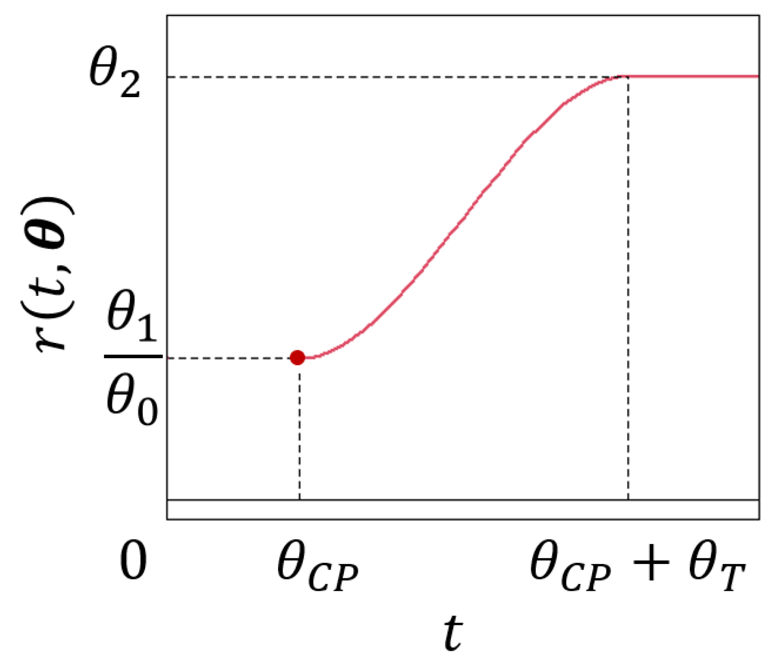
The family of solutions obtained by solving this simple DE is determined from the specification of the rate function $r(t,\theta )$. In this study, a non-decreasing rate function as presented in Figure 1 is proposed. This specification of the rate function resembles the mean function corresponding to the BCR model where two straight lines are connected by a polynomial. However, the obtained mean function poses a different alternative.

Up to the point where the deterioration process begins, the rate of change is zero, which translates into a horizontal trajectory of the f function at the value ${\theta }_0$. Then there is a transition period where the rate begins to increase up to a maximum value where it stabilizes. From this moment on, the decay is proportional to the cognitive state. Equation (7) presents the components of the rate function:

$$r(t,\mathit{\theta })=\left\{\begin{array}{cc}{\theta }_1/{\theta }_0,\hfill & t={\theta }_{CP}\hfill \\ p_3\left(t\right),\hfill & {\theta }_{CP}<t\le {\theta }_{CP}+{\theta }_T\hfill \\ {\theta }_2,\hfill & t>{\theta }_{CP}+{\theta }_T.\hfill \end{array}\right.$$

(7)

As in the previous cases, the CP is modeled through the parameter ${\theta }_{CP}$. Additionally, a transition period (of length ${\theta }_T$) around the CP is considered. Lastly, $p_3\left(t\right)$ is a polynomial of third degree that smoothly connects both parts of the rate function. To this end, it enforces the following constraints:

• $p_3\left({\theta }_{CP}\right)={\theta }_1/{\theta }_0$
• $p_3^{\prime }\left({\theta }_{CP}\right)=0$
• $p_3({\theta }_{CP}+{\theta }_T)={\theta }_2$
• $p_3^{\prime }({\theta }_{CP}+{\theta }_T)=0.$

The coefficients of this polynomial can be found solving a linear system (see Appendix A). It is important to note that the cubic polynomial $p_3\left(t\right)$ used to define the transition in the rate function does not introduce additional free parameters into the model. Instead, its four coefficients are entirely determined by the continuity and differentiability constraints imposed at the boundaries of the transition period. Therefore, the polynomial serves strictly as a smooth interpolant ensuring a gradual change in the rate function, and does not contribute additional flexibility in terms of parameter estimation. As a consequence, the number of parameters estimated in the DEM remains comparable to that of the other models considered. Under this specification, it is possible to obtain the closed analytical expression for the $f_{DEM}(.)$ function presented in Equation (8)

$$f_{DEM}(t,\mathit{\theta })=\left\{\begin{array}{cc}{\theta }_0+{\theta }_1\left(t-{\theta }_{CP}\right),\hfill & t\le {\theta }_{CP}\hfill \\ {\theta }_0{e}^{-{\int }_{{\theta }_{CP}}^{t}r(s,\mathit{\theta })ds},\hfill & t>{\theta }_{CP}.\hfill \end{array}\right.$$

(8)

After expanding the expression in the first part of Equation (8), ${\theta }_0-{\theta }_1{\theta }_{CP}$ could be thought as an intercept like parameter for the linear segment before the CP. Applying straightforward algebra, it is possible to expand the exponential expression in (8) as follows:

$$\left\{\begin{array}{cc}{\theta }_0{e}^{-{\mathcal{P}}_3\left(t\right)},\hfill & {\theta }_{CP}<t\le {\theta }_{CP}+{\theta }_T\hfill \\ {\theta }_0{e}^{-{\mathcal{P}}_3({\theta }_{CP}+{\theta }_T)+{\theta }_2(t-{\theta }_{CP}-{\theta }_T)},\hfill & t>{\theta }_{CP}+{\theta }_T.\hfill \end{array}\right.$$

(9)

Being ${\mathcal{P}}_3\left(t\right)={\int }_{{\theta }_{CP}}^t{p}_3\left(s\right)$. Additionally, by redefining ${\overline{\theta }}_0={\theta }_0{e}^{-{\mathcal{P}}_3({\theta }_{CP}+{\theta }_T)}$, the structure of the exponential decay becomes clearer.

Nonetheless, we prefer to present the model by means of Equations (6) and (7) since they provide a clearer interpretation of the parameters.

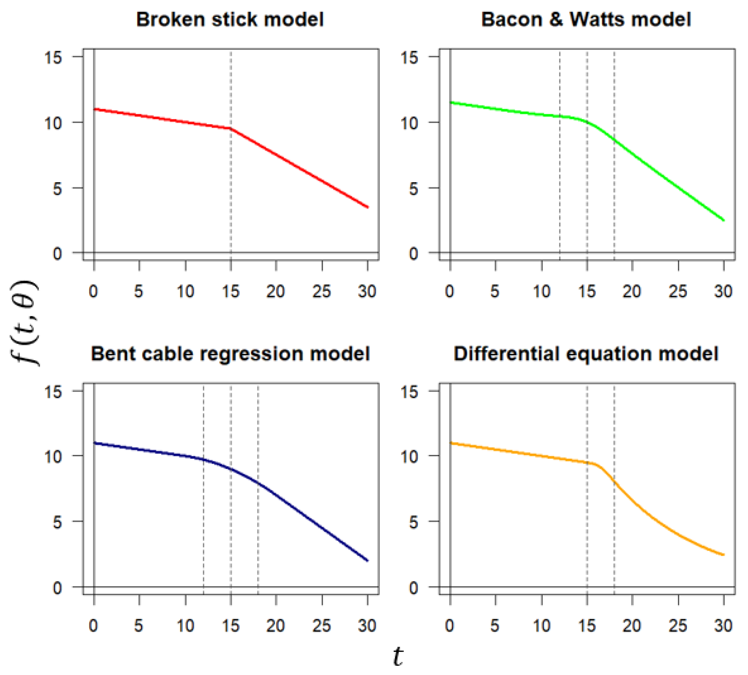
To better understand how these models work, Figure 2 compares the mean trajectory of the four alternatives presented in Equations (3)–(6).

Figure 2 shows how the four models consider three phases in the mean function. The BSM consists of two linear segments with different slopes abruptly joined at the CP. The other alternatives adhere to this pattern, adding a “transition” phase between.

Regarding the transition parameter, it has different meanings in the four models. In the BWM, its meaning is not trivial, but a “radius of curvature” (see page 528 of ref. [14]) can be constructed around the CP allowing for a smoother transition between both regimes. The BSM can be viewed as a limiting case of the BWM when the transition parameter equals zero, resulting in an abrupt transition. In the case of the BCR, the transition parameter represents the semi-amplitude of the transition period around the CP. Finally, in the DEM, it is the amplitude of the period that connects both the linear and the decay phases. This period starts at the CP and ends at beginning of the decline phase.

The DEM has the advantage that the value of the function $f_{DEM}$ is never less than zero. This property may be advantageous in applications where the response variable is inherently non-negative, such as cognitive scores. Additionally, as seen in Figure 2, is the only specification capable of capturing a non-linear behavior after the CP. The latter is relevant since, as will be presented in scenarios based on Monte Carlo simulation, an inappropriate choice at CP model selection could result in significant biases in estimating the CP.

2.3. Bayesian Inference

Due to the inclusion of random effects, a CP and the specification of a transition parameter, the proposed DEM belongs to the family of non-linear models and requires iterative and computationally demanding estimation methods. Hence, we opted for the use of a Bayesian estimation approach, that can better handle a (possibly) large number of random effects without resorting to numerical methods to solve high-dimensional integrals [21]. As we will see below, the estimation techniques were based on efficient Markov chain Monte Carlo (MCMC) algorithms.

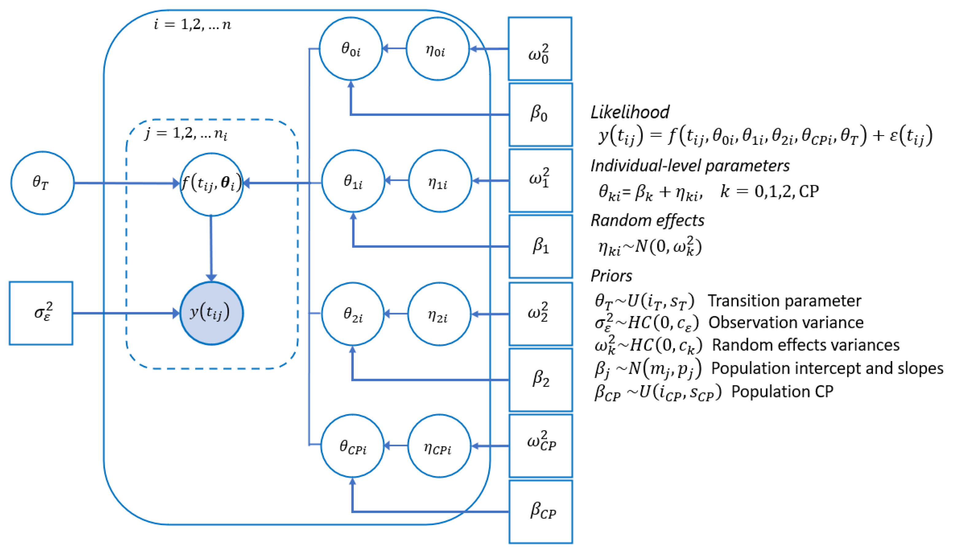
We selected the following prior distributions. We assigned non-informative Gaussian priors to the fixed effects with precision parameters set to 0.001. On the other hand, for the CP and the transition parameter we propose uniform priors whose range accounted for the duration of the study. Finally, as suggested by [22,23], we assigned half-Cauchy distributions as a weakly informative prior for the parameters associated with the error and random effects variances. These choices allowed us to write the models described above as in Figure 3:

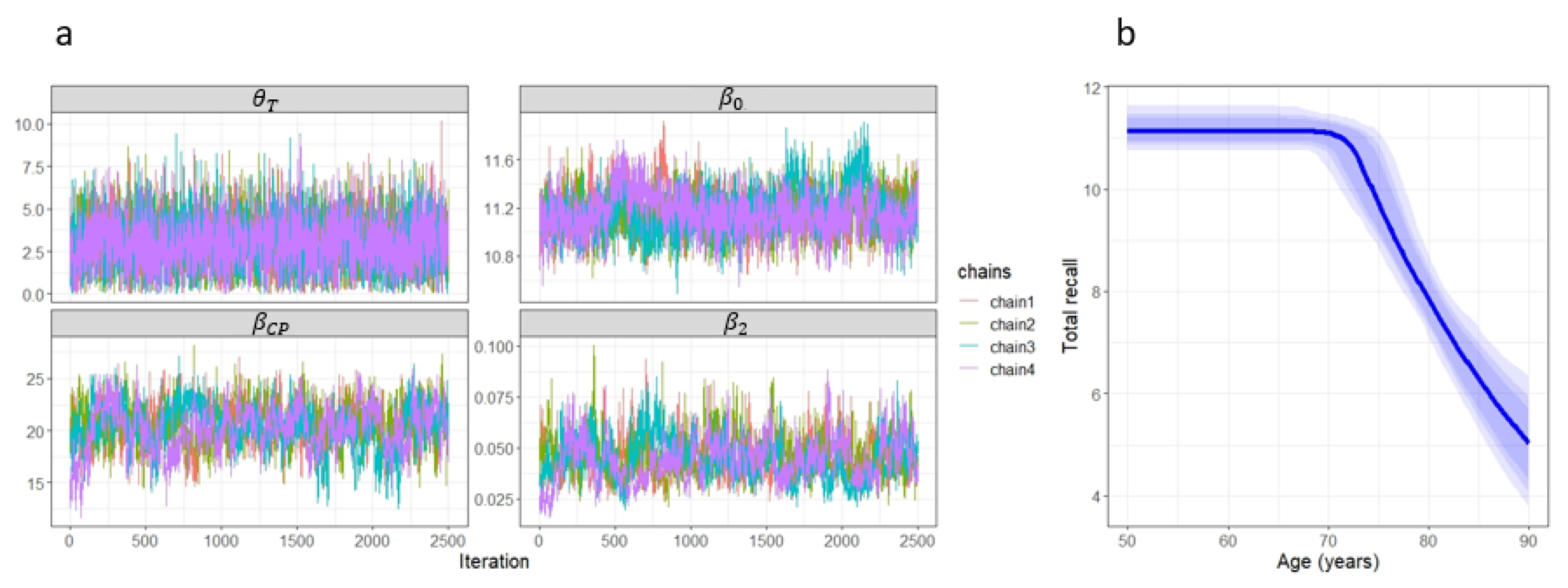
In all cases, we run four parallel Markov chains of model parameters for 5000 iterations each. After discarding the first 2500 iterations of each chain, we assess the convergence of the MCMC algorithm with the four separate Markov chain samples of size 2500. Convergence was monitored using the $\widehat{R}$ statistic, trace plots, and the effective sample size [24]. These checks were systematically applied in both the simulation study and the application to real-world data from ELSA. All statistical analyses were conducted using R [25] making use of the MCMC algorithms available in the rstan and rjags libraries [26,27].

2.4. Model Selection

One way to perform model selection within a Bayesian framework is by using the marginal likelihood [28]. In model selection, K competing models are considered and researchers are interested in the relative plausibility of each model ${\mathcal{M}}_k,k\in 1,2,\dots ,K,$ given the priors and the data. This relative plausibility is contained in the posterior model probability $p\left({\mathcal{M}}_k\right|y)$ of model ${\mathcal{M}}_k$ given the data:

$$p\left({\mathcal{M}}_k\right|y)={\displaystyle \frac{p\left(y\right|{\mathcal{M}}_k)p\left({\mathcal{M}}_k\right)}{{\sum }_{k=1}^{K}p\left(y\right|{\mathcal{M}}_k)p\left({\mathcal{M}}_k\right)}}$$

(10)

where $p\left(y\right|{\mathcal{M}}_k)$ is the marginal likelihood of the data under the ${\mathcal{M}}_k$ model. Thus, from the initial representation of modeling uncertainty contained in $p\left({\theta }_k\right|{\mathcal{M}}_k)$ and $p\left({\mathcal{M}}_k\right)$, the posterior distribution of the model $p\left({\mathcal{M}}_k\right|y)$ updates this uncertainty quantification after observing the data. For the applications considered in this study, the calculations necessary to compute these quantities were obtained using the algorithms of the bridgesampling R library [29].

In addition, another extensively used indicator is the widely applicable information criteria (WAIC) [30]:

$$\mathrm{WAIC}=-2\left\{{\displaystyle \sum _{i=1}^{n}log{\mathbb{E}}_{post}\left[p\left(y_i\right|\theta )\right]-\sum _{i=1}^n\mathbb{V}a{r}_{post}\left[logp\left(y_i\right|\theta )\right]}\right\}$$

(11)

where ${\mathbb{E}}_{post}$ and $\mathbb{V}a{r}_{post}$ represent the mean and variance with respect to the posterior distribution $p\left(\theta \right|y)$. Unlike posterior model probabilities, WAIC evaluates out-of-sample prediction accuracy. To this end, it uses the log-predictive density (which is a more general quantity than the mean squared error) and a bias correction that take into account the effective number of parameters. For the purposes of this study, the algorithms used to obtain the WAIC were those contained in the loo R library [31].

The fit indicators described above were introduced to assess the performance of the new DEM against BSM, BWM, and BCR. In this paper, the emphasis is on the better estimation of the CP. For this reason, the comparison is conducted in terms of bias and interval coverage. Lastly, to explore the overall fit of each model, the posterior model probabilities as well as the WAIC value are provided.

To accomplish this, we proposed three simulation-based experiments. The aim of these experiments is to compare the fit of the models in different situations and to determine their performance to estimate the CP. Finally, the performance of the DEM versus the other competitors is presented using real cognitive data from ELSA.

3. Simulation Study

We designed a simulation study based on three experiments. The first has the DEM as the data-generating process (DGP). In this case, not only is the DEM expected to present the best fit, but it is also expected to find negative biases in the other three model specifications when estimating the CP. The second scenario corresponds to a situation where the DGP is the BSM. We considered this scenario to assess how robust the DEM is when it is not the appropriate model. Finally, the third scenario is similar to the first one, but limiting the follow-up period after the CP so that the curvature of the trajectory is not sufficiently decisive to point to the DEM as the best model.

In all scenarios, we simulated 1000 data sets composed of 50 individuals observed on 10 occasions at random times between 0 and 20. The value of the parameter ${\beta }_1$ is set to 0, since the model is designed for application in studies of cognitive decline, where it is natural to assume that the cognitive state of the individuals remains constant until the moment when cognitive decline begins. This assumption is consistent with previous literature (e.g., Karr et al., 2018 [1]), which suggests cognitive performance remains relatively stable prior to decline. For this reason, each scenario considered a horizontal trajectory up to the CP, which was fixed in the middle of the follow-up period $({\beta }_{CP}=10)$. In Scenario 2, the slope after the CP $\left({\beta }_2\right)$ was set at $-0.5$, while Scenarios 1 and 3 considered a decline rate of $-0.5$. For all cases, the value of ${\beta }_0$ was set at 11, the observation noise had a variance ${\sigma }_{\epsilon }^2$ of $1.4$, and the random effects had variances of $0.3$, $0.1$, and 2 for the intercept, the slope (or rate), and the CP, respectively. Finally, the transition parameter (${\theta }_T$) was set to 3. The algorithm to generate the data sets follows the pseudo-code presented in Algorithm 1.

The parameters used in the simulation study were selected to reflect typical values observed in empirical cognitive aging research. In particular, the intercept value corresponds to the average total recall score observed among cognitively healthy older adults in the English Longitudinal Study of Ageing (ELSA) [32]. The post-decline rate was set to −0.5, representing a moderate deterioration compatible with prior studies, which report average annual declines in total recall scores ranging from 0.3 to 0.5 points [33]. This value was chosen to ensure that the change point is identifiable without being unrealistically steep. The remaining parameters were chosen to reproduce plausible levels of observation noise and inter-individual variability, and to allow for a meaningful transition period (${\theta }_T=3$) across different model specifications.

Algorithm 1 Data simulation for the s-th scenario.

Require: $N=1000;n_{obs}=50;n_{ij}=7;T_{max}=20;$ DGP parameters Ensure: N data sets 1: for $k\leftarrow 1$ to N do 2:      for $i\leftarrow 1$ to $n_{obs}$ do 1. Using a uniform distribution, generate 10 random times between 0 and $T_{max}$ ($t_{i1},t_{i2},\dots ,t_{i10}$). 2. Generate individual parameters from population-level Equation (2) using inputs and simulated random effects (see Figure 3) ${\theta }_{0i},{\theta }_{2i},{\theta }_{CPi}$. 3. Generate observations $y_{i1},y_{i2},\dots ,y_{i7}$ using the individual-level Equation (1). 3:      end for 4: end for

In each scenario, the four models considered were fitted to each of the 1000 data sets using the hierarchical Bayesian non-linear mixed model proposed in Figure 3. The choices of prior distributions could be observed in Appendix B (see

Table A1. Prior distributions for the simulation study described in Section 3. Note that N, U, and $HC$ denote the normal, uniform, and half-Cauchy distributions, respectively.

Parameter	Distribution	BSM	BWM	BCR	DEM	Description
Fixed effects
${\beta }_0$	$N(10,100)$	✓	✓	✓	✓	Intercept
${\beta }_2$	$N(0,100)$	✓	✓	✓	✓	Linear slope before CP (decay rate in DEM)
${\beta }_{CP}$	$U(0,20)$	✓	✓	✓	✓	Change point
${\theta }_T$	$U(0,5)$		✓	✓	✓	Transition parameter
Random effects
${\sigma }_{ϵ}^2$	$HC(0,10)$	✓	✓	✓	✓	Observation noise variance
${\omega }_{b_0}^2$	$HC(0,1)$	✓	✓	✓	✓	Intercept variance
${\omega }_{b_2}^2$	$HC(0,1)$	✓	✓	✓	✓	Slope (decay rate in DEM) variance
${\omega }_{b_{CP}}^2$	$HC(0,1)$	✓	✓	✓	✓	Change point variance

). Information on the posterior distribution of the parameters was extracted after verifying the convergence of the MCMC algorithm (see the distribution of the $\widehat{R}$ statistic and $n_{eff}$ for the ${\widehat{\beta }}_{CP}$ parameter in Figure A1 in Appendix C). The posterior median (PM) of the CP was used as the point estimator, and credibility intervals (CrI) were constructed using the 0.025 and 0.975 sample quantiles (higher posterior density intervals were also constructed but did not differ significantly from those reported in

Table 1. Results from the simulation experiments.

	Scenario 1	Scenario 2	Scenario 3
DGP	DEM	BSM	DEM
CP Estimate (95% CrI)
BSM	8.89 (7.96; 9.84)	9.98 (8.42; 11.56)	10.06 (9.31; 10.91)
BWM	9.23 (7.84; 16.13)	11.86 (8.65; 13.38)	10.49 (9.08; 18.78)
BCR	9.20 (7.97; 15.58)	10.91 (9.11; 13.82)	9.99 (9.34; 10.91)
DEM	10.40 (9.68; 11.24)	10.06 (8.50; 11.67)	10.56 (9.45; 14.17)
CP Bias (95% CrI)
BSM	−1.11 (−2.04; −0.16)	−0.02 (−1.58; 1.56)	0.06 (−0.69; 0.91)
BWM	−0.77 (−2.16; 6.13)	1.86 (−1.35; 3.38)	0.49 (−0.92; 8.78)
BCR	−0.80 (−2.03; 5.58)	0.91 (−0.89; 3.82)	−0.01 (−0.66; 0.91)
DEM	0.40 (−0.32; 1.24)	0.06 (−1.50; 1.67)	0.56 (−0.55; 4.17)
CP Effective Coverage (95% CrI)
BSM	0.25 (0.18; 0.31)	0.92 (0.89; 0.96)	0.946 (0.92; 0.98)
BWM	0.18 (0.13; 0.23)	0.79 (0.73; 0.84)	0.817 (0.76; 0.87)
BCR	0.25 (0.19; 0.31)	0.90 (0.86; 0.94)	0.952 (0.92; 0.98)
DEM	0.92 (0.88; 0.96)	0.95 (0.92; 0.98)	0.849 (0.80; 0.90)
Posterior Model Probability
BSM	<0.001	0.25	0.09
BWM	<0.001	0.19	0.11
BCR	<0.001	0.26	0.07
DEM	>0.99	0.31	0.73
WAIC (SE)
BSM	1841.83 (30.50)	1651.82 (29.38)	1670.53 (30.85)
BWM	1829.44 (30.31)	1653.00 (29.37)	1670.10 (30.70)
BCR	1842.73 (30.29)	1652.69 (29.44)	1671.69 (30.85)
DEM	1666.15 (26.61)	1658.81 (29.31)	1657.94 (30.34)

). The performance of the four models in estimating CP was evaluated through the bias of the ${\beta }_{CP}$ estimate, calculated as the difference between the real value and its corresponding estimate. It was considered that a successful (unbiased) estimation should include zero within the CrI of the bias. Likewise, using the CrI of ${\beta }_{CP}$ obtained in each of the 1000 data sets (as well as the true value of the CP), the effective coverage of this parameter was approximated in all models for each scenario. In this case, it is desirable that these values be as close as possible to 95%. Additionally, the values obtained from the posterior distribution of the parameters of each model were used to calculate posterior model probabilities and WAIC (and its standard error). We followed the pseudo-code presented in Algorithm 2 to obtain estimates, intervals, and fit indicators from every data set.

Algorithm 2 Data simulation for the sth scenario.

Require: N simulated data sets Ensure: bias, effective coverage, and posterior probabilities 1: for $k\leftarrow 1$ to N do 1. Fit $BSM$, $BWM$, $BCR$ and $DEM$ to data set k. 2. Get PM and 95% CrI of CP. 3. Compute fit indicators. 2: end for Summarize values obtained in c).

Table 1 presents the PM and the 95% CrI for the CP parameter, its bias, and the effective coverage probability of CrI. Finally, posterior model probability and WAIC are presented for the four models in each scenario.

The results presented in Table 1 suggest that the DEM has a superior performance when the decline after the CP shows enough curvature (Scenario 1). This can be seen in the posterior model probability, the lowest value of the WAIC estimate, on the unbiased nature of the CP estimator (the credible interval for the bias covers the value zero without being too wide), and on the effective posterior coverage probability of the credible interval of the true CP being very close to the nominal value of 95%. Furthermore, the performance of the BSM is suboptimal, as it exhibits a negative bias in the estimation of the CP.

In addition, it can be observed that in the other two scenarios, the DEM performance competes with the other alternatives, even in the worst case (Scenario 2). If the true decline is either linear (Scenario 2) or close to linear (Scenario 3), the CP estimated has a negligible median bias and a high posterior coverage close to the true CP value. It is worth noting that, even when the post-CP curvature is not sufficiently pronounced (Scenario 3), the posterior model probability indicates moderate evidence in favor of DEM.

4. Application

4.1. Data

ELSA is a prospective, population-based cohort of individuals aged over 50 to understand different aspects of aging in England [19]. The cohort was established in 2002 with data collected biannually across nine monitoring waves, in which interviews have been conducted with 19,221 individuals. Computational constraints led us to analyze a randomly selected subset of 5000 participants from ELSA. We focus on a memory marker, which is called the total word recall test [34]. This was constructed as the sum of both immediate and delayed recall tests. Participants were presented with a list of ten words and prompted to recall them immediately and after approximately five minutes. This test serves as a measure of verbal skills and working memory.

4.2. Results

Figure 4a depicts a spaghetti plot of the total recall test score versus age over a sample of 5000 randomly selected participants. Additionally, Figure 4b displays some highlighted trajectories in black over the light gray trajectories from the first panel. Although Figure 4a suggests significant variability among trajectories, a “stable” phase followed by a “downward” phase beginning between 60 and 70 years of age can be discerned. This pattern is also evident in Figure 4b, where individual trajectories vary in level but consistently show that the rate of change differs between the beginning and the end of the follow-up period.

We fitted the four models introduced in the change-point models section and calculated the model selection criteria presented in the model assessment section. Model hyperparameters matched those used in our simulation study (Appendix B, Table A1), with one key adaptation: the change-point parameter (${\beta }_{CP}$) was assigned a uniform (60, 80) prior for the ELSA application, reflecting both the cohort’s age distribution (baseline range: 50–90 years) and clinical evidence that cognitive decline onset rarely occurs outside this window. All other priors remained unchanged.

Table 2. Parameter estimates, 95% credible intervals, and model selection indicators.

BSM	BWM	BCR	DEM
Fixed Effects
${\beta }_0$	11.29	11.28	11.31	11.22
	(11.19; 11.40)	(10.17; 11.39)	(11.20; 11.42)	(11.11; 11.32)
${\beta }_2$	−50.26	−0.12	−0.26	−0.05
	(−0.29; −0.24)	(−0.14; −0.11)	(−0.28; −0.23)	(−0.06; −0.04)
${\beta }_{CP}$	68.61	67.77	68.33	74.28
	(67.30; 70.50)	(66.14; 69.20)	(66.85; 69.94)	(72.93; 75.60)
${\theta }_T$		3.33	2.47	3.63
		(0.26; 4.95)	(0.13; 4.82)	(0.69; 4.96)
Random Effects
${\sigma }_{ϵ}$	2.27	2.27	2.27	2.24
	(2.24; 2.30)	(2.25; 2.30)	(2.25; 2.30)	(2.22; 2.27)
${\sigma }_{{\beta }_0}$	2.12	2.13	2.13	2.16
	(2.05; 2.20)	(2.05; 2.20)	(2.06; 2.20)	(2.08; 2.32)
${\sigma }_{{\beta }_2}$	0.11	0.06	0.11	0.03
	(0.09; 0.13)	(0;05; 0.07)	(0.09; 0.14)	(0.02; 0.04)
${\sigma }_{{\beta }_{CP}}$	6.84	6.68	6.74	8.39
	(6.05; 7.80)	(5.81; 7.49)	(5.86; 7.61)	(7.74; 9.09)
Model Selection
WAIC	1,233,242.5	123,265.3	123,223.6	122,827.6
PMP	0.229	0.228	≤0.001	0.542

presents the estimated parameters, including posterior medians and credible intervals, as well as model selection indicators for the three baseline models—BSM, BWM, and BCR—and the proposed DEM. On the one hand, all four models agree on the average intercept and the random components estimates. However, although the posterior model probability provides only anecdotal evidence in favor of DEM, the value of WAIC favors it as well. We confirm that all model estimates presented in this section met standard convergence criteria across the four models compared.

Figure 5 compares the posterior distributions of the CP estimates across the four models, revealing critical differences in their characterization of cognitive decline onset. While the BSM, BWM, and BCR models converge on earlier CP estimates (medians: 67–68 years), the DEM suggests a markedly later onset (median: 74.3 years; 95% CrI: 72.9–75.6). This discrepancy aligns with our simulation results, where the DEM avoided the downward bias exhibited by other models when true decline was non-linear. The DEM’s wider credible intervals (2.7 years vs. 1–3 years in other models) reflect its capacity to capture individual variability in non-linear trajectories—a biologically plausible feature absent in piecewise-linear alternatives. Clinically, this 6-year shift in estimated onset could significantly impact intervention timing, as earlier estimates may prompt premature interventions, whereas the DEM’s later estimates better match the observed preservation of cognitive function in aging populations. These findings underscore the DEM’s advantages in both statistical rigor and translational relevance.

As seen in the simulation experiments, this could be due to non-linearities on the mean trajectory. Additionally, the DEM presents a narrower transition period, which is compensated by a higher variability in the random component of the CP.

The results obtained from the empirical application reveal greater discrepancies between models in estimating the change point (CP), which may stem from various factors—most notably, the presence of nonlinear dynamics that simpler models fail to capture adequately. Unlike the simulated data, the estimates reported in Table 2 exhibit divergence not only in the CP but also in the parameters associated with random effects and measurement error.

Finally, using the simulated values from the posterior distribution of the parameters from the DEM, Figure 6 presents trace plots from the fixed effects of the DEM and the fitted curve along a 95% probability band for total recall.

5. Conclusions

This paper introduced a non-linear alternative based on a new DEM specification to commonly used CP models and presented its performance compared to the models most commonly used in the literature. Model fitting was performed in a Bayesian context within the R framework using the $rjags$ or $rstan$ libraries. For the purposes of this study, model estimation using $rjags$ resulted in shorter runtimes than those required by $rstan$. Nevertheless, parameter estimation could also be undertaken straightforwardly within a frequentist framework. Comparison among models was conducted by computing model selection indicators that rely on the MCMC samples.

Different simulation scenarios were implemented to explore the performance of the DEM with reference to the BSM, BWM, and BCR models. From the analysis of the results of the simulation design, we observed that, when the cognitive decline phase had a sufficiently pronounced curvature, the DEM presented the best fit and produced a less biased estimator for the CP with higher posterior coverage in the credible interval. However, when there were not enough observations in the period where the curvature manifests itself, the performance of the DEM decreased. Furthermore, when the DGP did not exhibit curvature in the post-CP phase, the performance of DEM was found to be on par with that of its competitors.

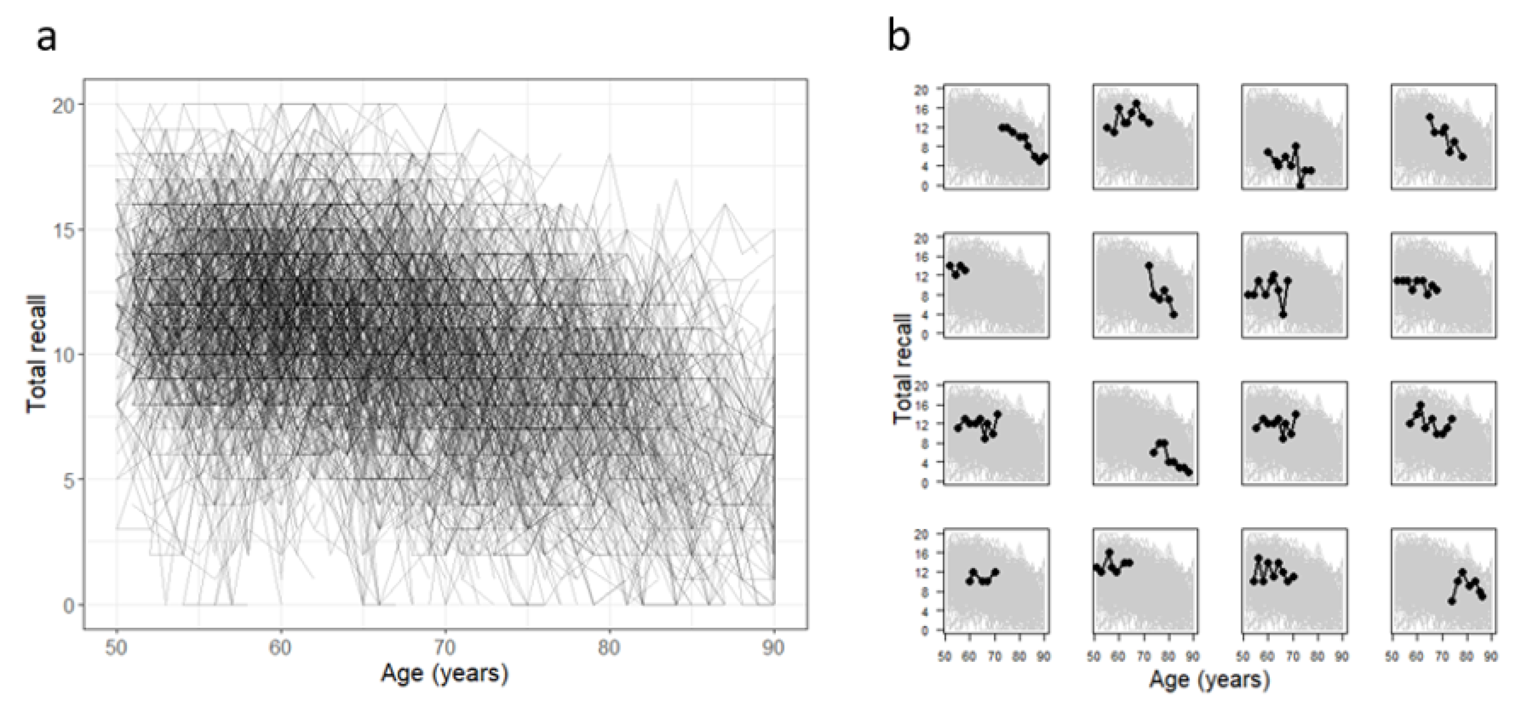
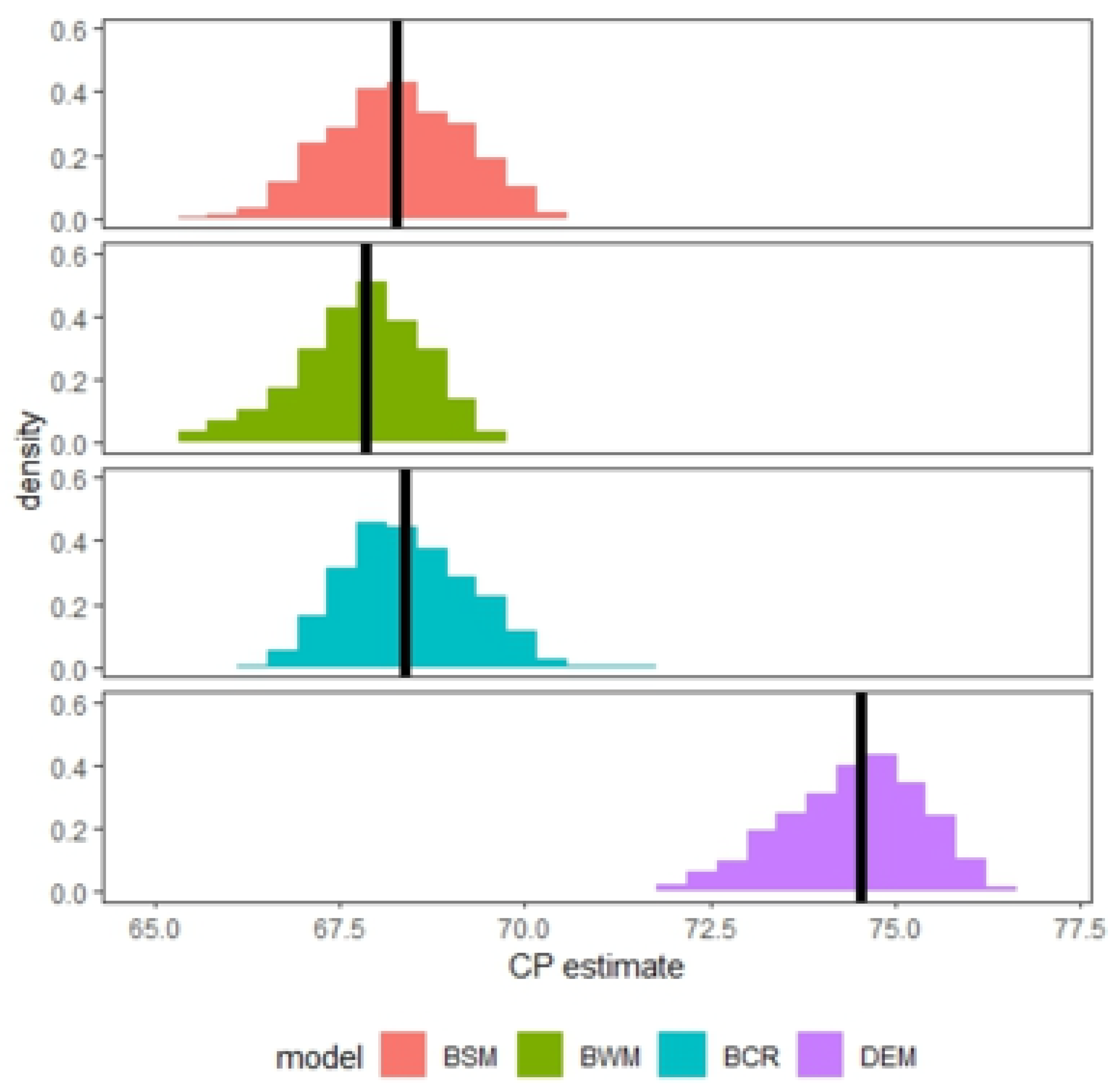
Ultimately, in the illustration of the models, we used actual cognitive data from the ELSA study. The results showed a slightly better fit of the DEM, which suggested an onset of the cognitive decline stage an average of 6 years later than the other models. This result is of particular interest in the area of aging because it provides vital information for health policy planning. In conclusion, it is worth noting that the model described in this paper is not meant to replace the models proposed in the literature, but rather to serve as a viable alternative, offering commendable statistical properties, transparent parameter interpretation, and biologically plausible features (such as the mean function consistently avoiding intersection with the x-axis). Regarding its use, it should be preferred when there are reasons to include non-linear behavior in the modeling stage.

Future research will focus on (1) extending the DEM to incorporate explanatory variables (e.g., genetic risk factors) and handle missing data patterns common in longitudinal aging studies, (2) developing open-source software tools to facilitate clinical adoption, (3) applications to other neurodegenerative processes, and (4) personalized intervention timing based on model-derived decline trajectories. These developments will further bridge statistical innovation with clinical practice in aging research.