Article

Proximal Causal Inference for Censored Data with an Application to Right Heart Catheterization Data

1
School of Management, Zhejiang University, Hangzhou 310058, China
2
Center for Data Science, Zhejiang University, Hangzhou 310058, China
*
Author to whom correspondence should be addressed.
Stats 2025, 8(3), 66; https://doi.org/10.3390/stats8030066
Submission received: 19 May 2025 / Revised: 14 July 2025 / Accepted: 19 July 2025 / Published: 22 July 2025
(This article belongs to the Section Applied Statistics and Machine Learning Methods)

Abstract

In observational causal inference studies, unmeasured confounding remains a critical threat to the validity of effect estimates. While proximal causal inference (PCI) has emerged as a powerful framework for mitigating such bias through proxy variables, existing PCI methods cannot directly handle censored data. This article develops a unified proximal causal inference framework that simultaneously addresses unmeasured confounding and right-censoring challenges, extending the proximal causal inference literature. Our key contributions are twofold: (i) We propose novel identification strategies and develop two distinct estimators for the censored-outcome bridge function and treatment confounding bridge function, resolving the fundamental challenge of unobserved outcomes; (ii) To improve robustness against model misspecification, we construct a robust proximal estimator and establish uniform consistency for all proposed estimators under mild regularity conditions. Through comprehensive simulations, we demonstrate the finite-sample performance of our methods, followed by an empirical application evaluating right heart catheterization effectiveness in critically ill ICU patients.

1. Introduction

In observational causal inference studies, the data we collect often serve as essential yet imperfect foundations for drawing causal conclusions. Classical estimation strategies rest on several key assumptions—such as the stable unit treatment value assumption (SUTVA) and positivity—but the most tenuous of these is the assumption of no unmeasured confounding. This condition requires that, once we stratify or adjust on observed covariates, treatment and control groups are rendered comparable. In practice, however, this hinges on the untestable premise that we have measured every variable that jointly influences both treatment assignment and outcome.
Any unmeasured confounding that remains threatens the validity of our causal estimates. Attempting to confirm the no-unmeasured-confounding assumption leads to circular reasoning: we would need to know the very hidden factors whose existence we are trying to rule out. Consequently, omitted variables continue to pose a persistent threat, even in well-designed observational studies.
This epistemological barrier has driven the development of methods designed to correct for measurement error and latent confounding. Contemporary causal methodology employs diverse strategies to mitigate bias from latent confounders, including sensitivity analysis [1,2], instrumental variable (IV) approaches [3,4,5,6,7], and recently proposed proximal causal inference [8,9,10]. Observational data inherently limit our capacity to fully validate the completeness of confounding mechanisms encoded in measured variables; thus, we can at most hope they are imperfect proxies of the unmeasured confounders. Holding this faith, the proximal approach exploits the proxy mechanism by positing two types of “bridge” functions—one linking proximal covariates to the outcome (outcome-inducing bridges, as in [8,9]) and the other linking covariates to treatment assignment (treatment-inducing bridges, as in [10,11]). Under suitable conditions on these bridge functions, it becomes possible to identify the true average causal effect despite the presence of unobserved confounding.
While tremendous success has been seen in the area of proximal causal inference since proposed by ([11,12,13,14,15,16,17,18,19,20,21,22,23,24] and many others), their application to survival data—which simultaneously features right-censoring and latent confounding—remains limited. A leading example is the evaluation of right heart catheterization (RHC) in critically ill patients [25,26]. Despite its long-standing clinical use since 1970, RHC’s effect on critically ill patients remains controversial [27]. Although several large observational studies have reported higher 30-day mortality among patients receiving RHC—even after adjusting for measured covariates [27,28,29]—these analyses are vulnerable to two key sources of bias: First, unmeasured confounding remains a concern: patients with more severe heart conditions are both more likely to undergo RHC and more prone to adverse outcomes, and existing control variables may omit critical indicators of illness severity [26]. Second, the restriction to 30-day mortality introduces censoring bias, since any late-onset benefits or harms of RHC remain unobserved beyond that window. Recent applications of proximal causal inference [25,26] address unmeasured confounding in this context but remain limited by restrictive linear hazard models or assumptions of fully observed outcomes, highlighting unresolved challenges for survival analysis with censored data.
To overcome these gaps, we propose a unified proximal inference approach that simultaneously handles unmeasured confounding and censored data, enabling more reliable estimation of RHC’s long-term effects. Our work bridges a critical methodological gap by extending proximal causal inference to settings with both right-censored outcomes and unmeasured confounding for average treatment effect (ATE) identification. We make two key contributions: First, we propose a proximal causal framework for right-censored data, enabling consistent estimation of average treatment effect (ATE) under unmeasured confounding. Second, by unifying the censored-outcome bridge function and the treatment confounding bridge function, we derive a proximal robust estimator and prove the consistency of all resulting estimators. Crucially, this robust estimator remains valid if either the treatment or the outcome bridge function is correctly specified—without requiring knowledge of which model is accurate.
The paper is structured as follows. In Section 2, we first review proximal identification results for average treatment effect (ATE) before extending this framework to derive identification conditions for censored outcomes. Building on these results, we develop three corresponding estimators based on: (i) the outcome bridge, (ii) the treatment bridge, and (iii) a combination of both bridges. Section 3 establishes the consistency properties of these proposed estimators under mild regularity conditions. To validate our approach, Section 4 presents simulation studies demonstrating the method’s ability to correct for unmeasured confounding bias. Section 5 implements the framework in the SUPPORT study on right heart catheterization, yielding new insights into RHC’s impact on long-term survival. All technical proofs are provided in the Appendix A, Appendix B, Appendix C, Appendix D and Appendix E

2. Methodology

2.1. Preliminaries

We commence by introducing the proximal causal inference (PCI) framework, which addresses confounding bias in the presence of unmeasured confounders affecting both treatment assignment and outcomes. While measured covariates alone cannot fully adjust for such confounding, PCI leverages proximal proxies to account for latent confounding mechanisms. This section formalizes the key components and identification assumptions of this framework.
Let the observed data consist of n independent and identically distributed (i.i.d.) observations of the form ( T , A , L ) , where: T denotes the true survival time, A is a binary treatment variable, and L represents a set of pre-exposure covariates. Following the approach of [9,10], we partition L into three mutually exclusive subsets:
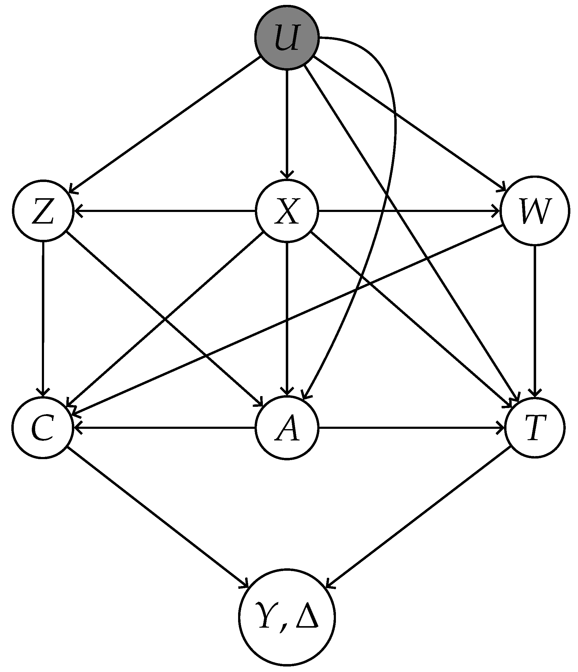
  • X: Measured common causes of both treatment A and outcome T.
  • Z: Treatment-inducing confounding proxies—causes of A confounded with T exclusively through unmeasured confounder U.
  • W: Outcome-inducing confounding proxies—causes of T confounded with A exclusively through U.
Let T ( a ) represent the potential survival time when the subject is assigned to treatment a, with a taking values in 0 , 1 .
Our primary target estimate is the average treatment effect (ATE):
ψ = E [ T ( 1 ) T ( 0 ) ] .
To establish nonparametric identification of ψ , we impose the following proximal relevance conditions:
Assumption 1
(Consistency). T = T ( A ) almost surely.
Assumption 2
(Positivity). 0 < Pr ( A = 1 | U , L ) < 1 almost surely.
Assumption 3
(Conditional Independence). The following conditional independence holds:
1. 
( Z , A ) and ( W , T ( a ) ) are conditionally independent given ( X , U ) , that is, ( Z , A ) ( W , T ( a ) ) | X , U .
2. 
T and Z are conditionally independent given ( X , U , A ) , that is, T Z | X , U , A .
Assumption 4
(Completeness). For any square-integrable function g and values a , x :
1. 
E [ g ( U ) | W , A , X ] = 0 g ( U ) = 0 almost surely.
2. 
E [ g ( W ) | Z , A , X ] = 0 g ( W ) = 0 almost surely.
3. 
E [ g ( U ) | Z , A , X ] = 0 g ( U ) = 0 almost surely.
4. 
E [ g ( Z ) | W , A , X ] = 0 g ( Z ) = 0 almost surely.
Assumption 1 represents a conventional consistency condition in the causal inference literature. Assumption 2 implies that the conditional probability of any exposure level given U and L is always greater than zero. Assumption 3 establishes that: (1) the proxy variables Z and W influence each other and the potential outcome T ( a ) only through their mutual dependence on X and U; and (2) Z affects the outcome T solely through its relationship with the unmeasured confounder U and the treatment A. This assumption relaxes the no unmeasured confounder assumption in causal inference literature by explicitly admitting the existence of unmeasured confounders [10]. The completeness Assumption 4 highlights the practical importance of collecting rich and relevant proxies. The first assumption in Assumption 4 ensures that the proxy variable W contains adequate information about the unmeasured confounder U; the second assumption in Assumption 4 guarantees that the proxy variable Z has sufficient variability to characterize the variation in W fully; the third assumption in Assumption 4 guarantees that Z’s variation is rich enough to account for the variation in U fully; the last assumption in Assumption 4 establishes that W’s variation must similarly be sufficient to completely capture Z’s variation.
Specifically, [8] showed that existence of an outcome confounding bridge function h ( W , A , X ) solving
E [ T h ( W , A , X ) | Z , A , X ] = 0
implies, under Assumptions 1–4, the counterfactual mean identification:
E [ T ( a ) ] = E [ h ( W , a , X ) ] .
Building on this result, [10] developed an alternative proximal identification framework. They proved that a treatment confounding bridge function q ( Z , A , X ) satisfying
E [ q ( Z , a , X ) W , A , X ] = 1 Pr ( A = a W , X )
yields, under Assumptions 1–4, the counterfactual mean identification:
E [ T ( a ) ] = E q ( Z , a , X ) Y I ( A = a ) .
In clinical trials with time-to-event outcomes such as survival times, complete data are often unavailable due to censoring, primarily caused by patient dropout. Formally, we define C as the censoring time, Y = min { T , C } as the observed survival time, and Δ = I ( T C ) as the event indicator (where Δ = 1 indicates an observed event without censoring). The available data consist of n independent and identically distributed (i.i.d.) samples { L i , A i , Y i , Δ i } i = 1 n , with L i = ( Z i , X i , W i ) . To enable valid statistical inference under right-censoring, we formalize a conditional independent censoring Assumption 5 to ensure valid statistical inference.
Assumption 5.
(Independent censoring) T and C are conditionally independent given ( Z , A , W , X ) , that is, T C | Z , A , W , X .
Assumption 5 represents a fundamental condition stating that the potential censoring time C and the time-to-event T are conditionally independent given the observed treatment A and covariates L. Assumption 5 is untestable; if violated, standard methods of estimating the conditional survival function for censoring will fail and lead to biased estimation. In the literature on informative censoring in survival analysis, a specific model is often imposed for modeling the relationship between survival time and censoring time. See [30] for more details.
Building upon this assumption, we implement the inverse probability of censoring weighting (IPCW) method [25,31] to handle censored data. The IPCW approach requires estimation of the conditional survival function for censoring:
S C ( t | A , L ) = Pr ( C > t | A , L ) .
In our implementation, we obtain these estimates through a standard Cox proportional hazards model, which remains the most widely used approach for modeling survival data due to its flexibility, robustness, and interoperability [32,33]. In addition, we include modern survival estimators (e.g., random survival forest [34]) in our data analysis to complement the Cox model. Figure 1 provides a possible directed acyclic graph (DAG) with conditional independence variables and censoring mechanism satisfying Assumptions 3 and 5.

2.2. Estimation Using Outcome Bridge

When dealing with censored data, the original nonparametric identification results developed by [8,9] for the proximal inference framework are no longer directly applicable. To address this limitation, we extend the proximal causal inference methodology to handle censored data scenarios, proposing novel identification strategies and corresponding estimation procedures for the average treatment effect (ATE).
We first examine the extension of [8]’s theoretical results to censored data settings. The central innovation systematically accounts for censoring time C in specifying the outcome bridge function h, which represents a fundamental advancement beyond current frameworks for properly handling right-censored outcomes.
Theorem 1.
Given the existence of an outcome confounding bridge function h ( W , A , X ) that solves (2), the results below hold under Assumptions 1–5:
1. The bridge function satisfies the orthogonality condition:
E Y h ( W , a , X ) · Δ S C ( Y Z , a , X , W ) | Z , A = a , X = 0 ,
2. The counterfactual mean outcome is identified as:
E [ T ( a ) ] = E h ( W , a , X ) · Δ S C ( Y Z , a , X , W ) .
The proof is given in the Appendix A. Through the outcome confounding bridge, Equation (2) takes the form of a Fredholm integral equation of the first kind, a characteristic feature of classical inverse problems. The existence conditions for solutions to such equations are established in [35]. Theorem 1 introduces a novel proximal identification framework for censored data settings. This result naturally leads to a two-stage estimation procedure: (i) Estimating the outcome confounding bridge h via Equation (6), which constitutes a Fredholm integral equation of the first kind under censored data; (ii) Constructing the corresponding estimator for ψ based on Equation (7).
Next, we consider estimation of the outcome confounding bridge function h. The existing literature provides multiple estimation approaches, including: the generalized method of moments implementation proposed by [8,10]; the neural network-based solution developed by [36]; and the kernel-based method introduced by [37]. Following the conditional moment restrictions established in Equation (2), we implement the generalized method of moments approach proposed by [10,25] for estimating the outcome confounding bridge function h in this study.
Specifically, we adopt a parametric specification for the function h ( W , A , X ) , defined as h ( W , A , X ; γ ) , where γ is a finite-dimensional parameter vector. The estimator γ ^ is obtained by solving the following empirical moment conditions:
E n Y h ( W , A , X ; γ ) Δ S C ( Y | Z , A , X , W ) K ( Z , A , X ) = 0 ,
where K ( Z , A , X ) is an arbitrarily chosen vector-valued function with dimensionality matching γ , and E n denotes the empirical expectation operator. Consequently, the average treatment effect estimator is given by:
ψ ^ h = E n h ( W , 1 , X ; γ ^ ) Δ S ^ C ( Y | Z , 1 , X , W ) h ( W , 0 , X ; γ ^ ) Δ S ^ C ( Y | Z , 0 , X , W ) .

2.3. Estimation Using Treatment Bridge

In the previous section, we demonstrated that outcome confounding bridge functions enable the nonparametric identification of counterfactual mean outcomes under censoring. Next, we generalize the approach of [10] by introducing a treatment confounding function q to formulate a Fredholm integral equation of the first kind for censored data settings. This provides an alternative identification result to Theorem 1, which avoids imposing moment restrictions on the outcome and can identify the distribution of potential outcomes. Here, we only focus on the mean of potential outcomes.
Theorem 2.
Given a treatment confounding bridge function q ( Z , A , X ) that solves (4), the counterfactual mean outcome is identifiable under Assumptions 1–5 through:
E [ T ( a ) ] = E q ( Z , A , X ) Y I ( A = a ) Δ S C ( Y | Z , A , X , W ) .
The proof is given in the Appendix B. An alternative proximal identification framework for censored data is established in Theorem 2, prompting a two-phase estimation: the bridge function q is first estimated by solving the first-kind Fredholm equation in (6), after which the causal estimator ψ is assembled using (7).
For estimating the treatment confounding bridge function q, we employ the same estimation framework used for h. The function q is modeled parametrically through q ( Z , A , X ; θ ) , with θ being a finite-dimensional parameter. The estimator is obtained by solving the following empirical estimating equation:
E n q ( Z , A , X ; θ ) M ( W , A , X ) M + ( W , A , X ) = 0 ,
where M ( W , A , X ) being any user-specified vector-valued function whose dimension corresponds to that of θ , and M + ( W , A , X ) = M ( W , 1 , X ) + M ( W , 0 , X ) . The resulting estimator for q is obtained as q ^ = q ( Z , A , X , θ ^ ) . The average treatment effect estimator is then defined by:
ψ ^ q = E n Y q ( Z , 1 , X ; θ ^ ) Δ S ^ C ( Y | Z , 1 , X , W ) Y q ( Z , 0 , X ; θ ^ ) Δ S ^ C ( Y | Z , 0 , X , W ) .

2.4. Estimation Using Both Bridges

Clearly, when all conditions from Assumptions 1–5 hold, the average treatment effect ψ can be identified through either h or q. This motivates us to develop a robust estimator for ψ .
Theorem 3.
Assume there exist two bridge functions: an outcome confounding bridge function h ( W , A , X ) that solves the integral Equation (2), and another bridge function q ( Z , A , X ) that satisfies the integral Equation (4). Then, under Assumptions 1–5, the counterfactual mean outcome is identified as:
E [ T ( a ) ] = E I ( A = a ) q ( Z , A , X ) [ Y h ( W , A , X ) ] + h ( W , A , X ) Δ S C ( Y | Z , A , X , W ) .
The proof is given in the Appendix C. Given the aforementioned two estimators, we define a new estimator
ψ ^ = E n [ ( ( 1 ) 1 A q ^ ( Z , A , X ) Y h ^ ( W , A , X ) + h ^ ( W , 1 , X ) h ^ ( W , 0 , X ) ) Δ S ^ C ( Y Z , A , X , W ) ] ,
where h ^ and q ^ can be estimated using the parametric bridge function estimators in [10]. To accommodate settings with more complex data structures—where the true bridge functions may be highly nonlinear or reside in rich function spaces—we propose a robust estimator based on a minimax formulation.
Building upon the minimax framework established by the literature [11,13,14,37], we formulate the nonparametric estimation of the outcome confounding bridge function h through the following optimization problem:
h ^ = arg min h H sup g G [ 1 n i = 1 n Y i h ( W i , A i , X i ) Δ S C ( Y Z , A , X , W ) g ( Z i , A i , X i )     μ 1 , n g G 2 g 2 , n 2 ] + μ 2 , n h H 2 ,
where μ 1 , n , μ 2 , n > 0 serve as regularization parameters controlling model complexity, and g 2 , n : = n 1 i = 1 n g 2 ( Z i , A i , X i ) denotes the empirical 2 norm. The function spaces H and G are appropriately chosen for modeling the outcome confounding bridge function h and its associated critic function g, respectively. These can be taken as reproducing kernel Hilbert spaces (RKHS), deep neural networks, or other flexible function classes that allow for nonparametric estimation while ensuring computational feasibility. The norms · H and · G correspond to their respective function spaces. We recommend using RKHS representations, as they are not necessarily computationally intensive and can provide closed-form solutions under certain conditions [13,38].
Similarly, we estimate the treatment confounding bridge function q through the following min–max optimization problem. For each treatment level a A , we define:
q ^ ( · , a , · ) = arg min q Q { sup f F [ 1 n i = 1 n I ( A i = a ) q ( Z i , a , X i ) 1 f ( W i , X i ) λ 1 , n f F 2 f 2 , n 2 ] + λ 2 , n q Q 2 } ,
where λ 1 , n , λ 2 , n > 0 are regularization parameters controlling model complexity. Q and F represent appropriately chosen function spaces for estimating the treatment confounding bridge function q and and its associated critic function f, respectively. As before, these may be taken as RKHS or other suitable nonparametric function classes. · Q and · F denote the native norms associated with their respective function spaces, and f 2 , n : = n 1 i = 1 n f 2 ( W i , X i ) is the empirical 2 norm.

3. Theoretical Results

In this section, we investigate the uniform convergence properties of the estimators ψ h , ψ q and ψ . To establish these theoretical properties, we first introduce the following assumptions.
Assumption 6.
The estimators h ^ ( W , A , X ) , q ^ ( Z , A , X ) , and S ^ C ( Y | A , L ) converge uniformly in probability to their respective deterministic limits h m ( W , A , X ) , q m ( Z , A , X ) , and S C m ( Y | A , L ) . That is,
sup W , A , X | h ^ ( W , A , X ) h m ( W , A , X ) | = o p ( 1 ) ,         sup Z , A , X | q ^ ( Z , A , X ) q m ( Z , A , X ) | = o p ( 1 ) ,         sup Y , A , L | S ^ C ( Y | A , L ) S C m ( Y | A , L ) | = o p ( 1 ) .
This assumption does not require that the estimators h ^ ( W , A , X ) , q ^ ( Z , A , X ) and S ^ C ( Y | A , L ) are consistent for the truth, only that they converge to fixed functions. In the next theorem, we show the consistency of the proposed three estimators ψ ^ h , ψ ^ q and ψ ^ .
Theorem 4
(Consistency). Under Assumptions 1–6, the following holds:
(i) 
If h m ( W , A , X ) = h ( W , A , X ) and S C m ( Y | A , L ) = S C ( Y | A , L ) , then ψ ^ h is a consistent estimator of ψ;
(ii) 
If q m ( Z , A , X ) = q ( Z , A , X ) and S C m ( Y | A , L ) = S C ( Y | A , L ) , then ψ ^ q is a consistent estimator of ψ;
(iii) 
If S C m ( Y | A , L ) = S C ( Y | A , L ) and either h m ( W , A , X ) = h ( W , A , X ) or q m ( Z , A , X ) = q ( Z , A , X ) holds, then ψ ^ is a consistent estimator of ψ.
The proof is given in the Appendix D. Theorem 4 demonstrates the consistency of estimators ψ ^ h , ψ ^ q , and ψ ^ for the parameter ψ under suitable regularity conditions. The combined estimator ψ ^ exhibits robustness: it remains consistent for ψ if either the treatment confounding bridge function q or the outcome confounding bridge function h is consistently estimated, without requiring both conditions to hold simultaneously.

4. Simulations

The simulation study employs a data-generating process (DGP) inspired by [10], who developed a proximal framework. Building on their semiparametric approach, we integrate proximal concepts with censoring mechanisms, adapting their core structure to address censored data scenarios. This extension reflects our novel combination of proximal inference and censoring in the research. Below we provide a concise overview of the adapted framework. To evaluate the performance of our proposed method, we consider the following three scenarios:
Case 1. The covariates X are generated from a multivariate normal distribution N ( Γ x , Σ x ) , where Γ x = ( 0 , 0 ) T and Σ x = 0.0625 0 0 0.0625 . The treatment variable A is then generated conditionally on X, following a Bernoulli distribution Bernoulli ( p A ) , where the success probability is given by
p A = [ 1 + exp { ( 0.125 , 0.125 ) T X } ] 1 .
Next, Z , W and U are generated from a multivariate normal distribution conditioned on A and X: ( Z , W , U ) A , X MVN ( μ , Σ ) , where the mean vector and covariance matrix are defined as:
μ = 0.25 + 0.25 A + 0.25 X 1 + 0.25 X 2 0.25 + 0.125 A + 0.25 X 1 + 0.25 X 2 0.25 + 0.25 A + 0.25 X 1 + 0.25 X 2 , Σ = 1 0.25 0.5 0.25 1 0.5 0.5 0.5 1 ,
The outcome Y is generated as the conditional expectation E ( Y | W , U , A , Z , X ) plus an independent normal noise term N ( 0 , 0.0625 ) . The conditional expectation is specified as:
E ( Y | W , U , A , Z , X ) = b 0 + b a A + b x X + ( b w ω ) E ( W | U , X , A ) + ω W ,
where
E ( W | U , X , A ) = μ 0 + μ x X + μ a A + σ w u σ u 2 ( U κ 0 κ a A κ x X ) .
The parameters are set as follows:
b 0 = 2 , b a = 2 , b x = ( 0.25 , 0.25 ) T , b w = 4 , μ 0 = 0.25 , μ a = 0.125 , μ x = ( 0.25 , 0.25 ) T , ω = 2 , κ 0 = 0.25 , κ a = 0.25 , κ x = ( 0.25 , 0.25 ) T .
We consider the following outcome confounding bridge function h and treatment confounding bridge function q:
h ( W , A , X ; b ) = b 0 + b a A + b w W + b x X ,
q ( Z , A , X , t ) = 1 + exp ( 1 ) 1 A t 0 + t a A + t z Z + t x X ,
with parameters t 0 = 0.25 , t z = 0.5 , t a = 0.125 and t x = ( 0.25 , 0.25 ) T .
The censoring time C is generated using the following hazard rate function:
λ C ( t | X 1 , X 2 ) = 16 t 3 exp { X 1 2 X 2 } .
Case 2. The settings are identical to Case 1, except for the following modifications: Z , W and U are generated from a multivariate normal distribution conditioned on A and X: ( Z , W , U ) A , X MVN ( μ , Σ ) , where the mean vector and covariance matrix are defined as:
μ = 0.25 + 0.25 A + 0.3 X 1 + 0.4 X 2 0.25 + 0.125 A + 0.3 X 1 + 0.5 X 2 0.25 + 0.25 A + 0.2 X 1 + 0.1 X 2 , Σ = 1 0.25 0.5 0.25 1 0.5 0.5 0.5 1 ,
Case 3. The data generation process remains identical to Case 1, with the following modifications: The variables Z , W and U are generated from a multivariate normal distribution conditioned on A and X: ( Z , W , U ) A , X MVN ( μ , Σ ) , where the mean vector and covariance matrix are respectively defined as:
μ = 0.25 + 0.25 A + 0.3 X 1 + 0.4 X 2 0.25 + 0.125 A + 0.3 X 1 + 0.5 X 2 0.25 + 0.25 A + 0.2 X 1 + 0.1 X 2 , Σ = 1 0.25 0.5 0.25 1 0.5 0.5 0.5 1 .
Additionally, the parameters are set as b a = 1 , b w = 3 .
We evaluate three proximal causal inference methods: proximal outcome regression, proximal inverse probability weighting, and proximal robust estimators. The confounding bridge functions h and q were estimated by solving the respective estimating Equations (8) and (11), producing the estimators h ^ and q ^ under models (15) and (16). The resulting estimators obtained from proximal outcome regression, proximal inverse probability weighting, and proximal doubly robust methods are denoted as ψ ^ h , ψ ^ q , and ψ ^ , respectively.
For benchmarking, we implemented two approaches. The first approach uses a standard doubly robust estimator ( ψ ^ DR ), which remains unbiased under exchangeability. The estimator takes the form:
ψ ^ DR = E n { ( ( 1 ) 1 A f ^ ( A L ) Y E ^ [ Y L , A ]         + E ^ [ Y L , A = 1 ] E ^ [ Y L , A = 0 ] ) · Δ S C ( Y Z , A , X , W ) } ,
where the propensity score f ^ ( A | L ) was fitted via logistic regression and the outcome model E ^ [ Y | L , A ] via linear regression.
The second approach utilizes machine learning through random survival forests (RSF) under the Metalearners framework [39], implemented in the R package (https://www.r-project.org/) randomForestSRC [40], to obtain the estimator ψ ^ r f . RSF nonparametrically estimates survival functions by aggregating predictions from survival-tree ensembles. It handles right-censored data through time-to-event-optimized splits and computes survival curves using terminal node estimators.
To assess performance, we examined four scenarios:
  • Correct specification: Using the original variables X and W for h, and X and Z for q.
  • Outcome bridge misspecification: Replacing W with a transformed variable W = | W | 1 / 2 + 3 in h.
  • Treatment bridge misspecification: Replacing Z with Z = | Z | 1 / 2 + 3 in q.
  • Double misspecification: Simultaneously substituting W = | W | 1 / 2 + 1 and Z = | Z | 1 / 2 + 1 in h and q.
For each scenario, the conventional robust estimator was also applied using the same transformed variables. Simulations used n = 500 observations and 500 Monte Carlo replicates per scenario.
Table 1, Table 2 and Table 3 present the simulation results for the three cases, where bias is defined as the systematic difference between an estimator’s expected value and the true parameter value. Mathematically, for an estimator ψ ^ of ψ , the bias is defined as: b i a s ( ψ ^ ) = E n ( ψ ^ ) ψ . The Mean Squared Error (MSE) of an estimator ψ ^ of ψ measures the average squared deviation of the estimator from the true value, defined as: M S E ( ψ ^ ) = E n ( ψ ^ ψ ) 2 . Consistent with theoretical expectations, the proximal IPW estimator ψ ^ q demonstrates minimal bias in Scenarios 1 and 2, while the proximal OR estimator ψ ^ h shows comparable performance in Scenarios 1 and 3. The proximal robust estimator ψ ^ maintains small bias across the first three scenarios. Under Scenario 4’s model misspecification conditions, all three proximal estimators ( ψ ^ q , ψ ^ h , and ψ ^ ) exhibit comparable bias magnitudes. Notably, both the conventional robust estimator and the random survival forests-derived estimator exhibit substantial bias across all scenarios, which can be attributed to unmeasured confounding effects.

5. RHC Data Revisited

We provide an empirical application using a medical dataset on the effects of right heart catheterization (RHC) originally derived from the Study to Understand Prognoses and Preferences for Outcomes and Risks of Treatments (SUPPORT) [28]. The RHC dataset is widely regarded as a benchmark in survival analysis because it features clinically meaningful time-to-event outcomes, substantial right censoring, rich covariate information, and nonrandomized treatment assignments. The likelihood of unmeasured confounding—such as physician discretion informed by subtle clinical indicators—makes this dataset a prototypical testbed for evaluating causal inference methods that relax the strict no-unmeasured-confounding assumption. Recent methodological advances in proximal causal inference have used the proxy structure of the RHC data to illustrate identification and estimation of treatment effects in the presence of latent confounders [8,9,10].
The original study included 5735 critically ill patients admitted to the intensive care unit (ICU) for specified disease categories at one of five U.S. teaching hospitals between 1989 and 1994. For each patient, the data include treatment status A (equals to 1 if RHC was performed within 24 h of admission), the survival time T, and several variables selected by critical care specialists, including demographic factors, comorbidities, diagnoses, and various laboratory values. We treat Δ = 1 as an indicator of observed death by time T.
Prior studies have found that RHC may have a harmful effect on 30-day survival among critically ill ICU patients and that this detrimental effect may be even larger when accounting for unmeasured confounding [9,10]. However, these results are limited to survival time censored at 30 days, which does not capture potential longer-term effects. In this paper, we instead focus on the full observed survival time under censoring to assess the long-term impact of RHC on patient outcomes.
Following [10,25], we set
Z = ( pafi 1 , paco 21 ) , W = ( ph 1 , hema 1 ) ,
and select same X as [25]. We adopt the outcome-confounding bridge function from Equation (6) and the treatment-confounding bridge function from Equation (10). Table 4 summarizes the key variables. The mean survival time Y is 163 days, with a maximum of 1351 days; 64.9% of patients died before censoring, and 35.1% were censored. We conduct a sensitivity analysis for the independent censoring assumption based on the imputation of missing failure times using a bootstrap approach [41]. The results in Figure A1 in the Appendix E indicate that the sensitivity parameter gamma does not affect the robustness of estimating the censor distribution with m = 20 imputed datasets. See [41] for more details about this sensitivity analysis.
To estimate the censoring distribution S C , we fit a random survival forest model [34]. After estimating the bridge functions, we compute our proposed estimators while accounting for censoring: the proximal outcome regression (POR) estimator, the proximal inverse probability weighting (PIPW) estimator, and the proximal robust (PR) estimator. We compare these with benchmark methods, including the censored standard doubly robust estimator (DR), the uncensored standard doubly robust estimator (UDR) proposed by [42], and the uncensored robust proximal estimator (UPCI) proposed by [10]. To estimate the confidence interval of these estimators, we apply a nonparametric bootstrap procedure following [23,43,44] with 200 replications. In each replication, we resample the data with replacement to match the original sample size.
Table 5 presents point estimates with 95% bootstrap confidence intervals. The proximal robust estimator (PR) suggests that RHC reduces patient survival by an average of 14 days. Relative to the proximal outcome estimator (POR) and proximal IPW estimators (PIPW), its confidence interval is appreciably narrower, indicating greater estimator stability. The extreme variability of the PIPW estimator stems from estimating the treatment confounding bridge function in Equation (4), since when Pr ( A = a | W , X ) is small, even minor estimation errors can greatly inflate the IPW weights.
When censoring is ignored (i.e., falsely treating Y as T), the 95% interval broadens and the estimated negative effect of RHC intensifies, implying that failing to account for censoring may underestimate uncertainty and mortality risk—consistent with [25]. Likewise, omitting unmeasured confounders may inflate RHC’s estimated mortality risk, in line with [26]. Finally, sensitivity analyses—sequentially dropping each proxy variable and varying the S C estimation—are reported in Table 6 and verify the above findings.

6. Discussion

This article presents a nonparametric identification framework for causal effects with right-censored outcomes within the proximal causal inference paradigm. We develop three innovative estimators of the average treatment effect that relax the conventional no-unmeasured-confounding assumption. Under mild regularity conditions, we establish uniform consistency for all proposed estimators. Notably, our combined estimator ψ ^ demonstrates a robust property, consistently estimating the average treatment effect when either the treatment confounding bridge function q or the outcome confounding bridge function h is correctly specified. Through extensive simulation studies and an empirical application to right heart catheterization (RHC) data, we demonstrate the practical utility of our methodology. Our findings reveal that RHC reduces patient survival by approximately 14 days on average, suggesting that existing literature may have systematically underestimated both the mortality risk and associated uncertainty of this procedure.
Several promising extensions warrant further investigation. First, while our current work addresses misspecification of bridge functions q and h, the impact of misspecified conditional survival functions for censoring times remains an important open question. Second, extending the proposed framework to time-varying treatment settings would significantly enhance its practical relevance. Third, although we have established consistency, characterizing the convergence rates and asymptotic distributions of our estimators represents a crucial direction for future theoretical work.

Author Contributions

Y.H.: methodology, software, writing—original draft preparation. Y.G.: conceptualization, validation, writing—review and editing. M.Q.: software, data curation, writing—original draft preparation, writing—review and editing, supervision. All authors have read and agreed to the published version of the manuscript.

Funding

The authors were supported by the National Key R&D Program of China (2024YFA1015600) and the National Natural Science Foundation of China (12471266 and U23A2064).

Institutional Review Board Statement

Not applicable.

Informed Consent Statement

Not applicable.

Data Availability Statement

The data supporting this research are publicly available at https://hbiostat.org/data/repo/rhc (accessed on 15 May 2025).

Conflicts of Interest

The authors declare no conflicts of interest.

Appendix A

Proof of Theorem 1.
We first show that
E [ ( Y h ( W , a , X ) ) Δ S C ( Y | Z , a , X , W ) | Z , A = a , X ] = 0 .
To show this, note that T C | Z , A , W , X , so we have that
E [ ( Y h ( W , a , X ) ) Δ S C ( Y | Z , a , X , W ) | Z , A = a , X ] = E [ E [ ( Y h ( W , a , X ) ) Δ S C ( Y | Z , a , X , W ) | Z , A = a , X , W ] | Z , A = a , X ] = E [ E [ T h ( W , a , X ) Δ S C ( Y | Z , a , X , W ) | Z , A = a , X , W ] | Z , A = a , X ] = E [ T h ( W , a , X ) ) | Z , A = a , X ] = 0 .
where the second equality is due to Assumption 5.
Note that
E [ Y Δ S C ( Y | Z , a , X , W ) | Z , A = a , X ] = E [ E [ Y Δ S C ( Y | Z , a , X , W ) | Z , A = a , X , W ] | Z , A = a , X ] = E [ T | Z , A = a , X ] = E [ E [ T | Z , A = a , X , U ] | Z , A = a , X ] = E [ E [ T ( a ) | A = a , X , U ] | Z , A = a , X ] ,
where the second equality is due to Assumption 5, the third equality is due to Assumption 1, and the last equality is due to Assumption 3.
For the term E [ h ( W , A , X ) Δ S C ( Y | Z , a , X , W ) | Z , A = a , X ] , we have
E [ h ( W , A , X ) Δ S C ( Y | Z , a , X , W ) | Z , A = a , X ] = E [ E [ h ( W , A , X ) Δ S C ( Y | Z , a , X , W ) | Z , A = a , X , W ] | Z , A = a , X ] = E [ h ( W , A , X ) | Z , A = a , X ] = E [ E [ h ( W , A , X ) | Z , A = a , X , U ] | Z , A = a , X ] = E [ E [ h ( W , A , X ) | A = a , X , U ] | Z , A = a , X ] ,
where the last equality is due to Assumption 3.
Following similar arguments as in Theorem 2.1 of [10], we now proceed to prove
E [ T ( a ) ] = E [ h ( W , a , X ) Δ S C ( Y | Z , a , X , W ) ] .
Note that
E [ ( Y h ( W , A , X ) ) Δ S C ( Y | Z , a , X , W ) | Z , A = a , X ] = E [ E [ T ( a ) | A = a , X , U ] | Z , A = a , X ] E [ E [ h ( W , a , X ) | A = a , X , U ] | Z , A = a , X ] = 0 .
By Assumption 4, we have
E [ T ( a ) | A = a , X , U ] E [ h ( W , a , X ) | A = a , X , U ] = 0 .
By Assumption 3,
E [ T ( a ) | A = a , X , U ] = E [ T ( a ) | X , U ] ,
and
E [ h ( W , a , X ) | A = a , X , U ] = E [ h ( W , a , X ) | X , U ] .
Therefore,
E [ T ( a ) ] = E [ E [ h ( W , a , X ) | X ] ] = E [ E [ E [ h ( W , a , X ) | Z , a , X , W ] | X ] ] = E [ E [ E [ h ( W , a , X ) Δ S C ( Y | Z , a , X , W ) | Z , a , X , W ] | X ] ] = E [ h ( W , a , X ) Δ S C ( Y | Z , a , X , W ) ] .

Appendix B

Proof of Theorem 2.
As a preliminary step, we prove the following key result:
        E [ I ( A = a ) Y q ( Z , A , X ) Δ S C ( Y | Z , A , X , W ) ] = E [ E [ I ( A = a ) Y q ( Z , A , X ) Δ S C ( Y | Z , A , X , W ) | Z , A , X , W ] ] = E [ I ( A = a ) q ( Z , A , X ) E [ Y Δ S C ( Y | Z , A , X , W ) | Z , A , X , W ] ] = E [ I ( A = a ) q ( Z , A , X ) E [ T | Z , A , X , W ] ] = E [ I ( A = a ) q ( Z , A , X ) T ]
where the third equality is due to Assumption 5. Following analogous arguments to those in the proof of Theorem 2.2 in [10], we now proceed to prove
E [ T ( a ) ] = E [ I ( A = a ) q ( Z , A , X ) T ] .
According to the proof of Theorem 2.2 in [10], we have
E [ q ( Z , a , X ) | U , A = a , X ] = 1 Pr ( A = a | U , X ) .
By Assumption 3,
        E [ I ( A = a ) q ( Z , A , X ) T | U , X ] = E [ q ( Z , A , X ) T | U , X , A = a ] Pr ( A = a | U , X ) = E [ T | U , X , A = a ] E [ q ( Z , A , X ) | U , X , A = a ] Pr ( A = a | U , X ) = E [ T | U , X , A = a ] = E [ T ( a ) | U , X ] .
Therefore, we have
E [ T ( a ) ] = E [ I ( A = a ) Y q ( Z , a , X ) Δ S C ( Y | Z , A , X , W ) ] .

Appendix C

Proof of Theorem 3.
Note that
E I ( A = a ) q ( Z , A , X ) [ Y h ( W , A , X ) ] + h ( W , A , X ) Δ S C ( Y | Z , A , X , W ) = E I ( A = a ) q ( Z , A , X ) [ Y h ( W , A , X ) ] Δ S C ( Y | Z , A , X , W ) + E h ( W , A , X ) Δ S C ( Y | Z , A , X , W ) = E E I ( A = a ) q ( Z , A , X ) [ Y h ( W , A , X ) ] Δ S C ( Y | Z , A , X , W ) | Z , A , X + E h ( W , A , X ) Δ S C ( Y | Z , A , X , W ) = E I ( A = a ) q ( Z , A , X ) E [ Y h ( W , A , X ) ] Δ S C ( Y | Z , A , X , W ) | Z , A , X + E [ T ( a ) ] = E [ T ( a ) ]
where the third and last equality can be derived by Theorem 1. □

Appendix D

Proof of Theorem 4.
(i) Recall that the average treatment effect estimator are defined as
ψ ^ h = E n [ h ^ ( W , 1 , X ) Δ S ^ C ( Y | Z , 1 , X , W ) h ^ ( W , 0 , X ) Δ S ^ C ( Y | Z , 0 , X , W ) ] .
Under Assumptions 6, let h m ( W , A , X ) and S C m ( Y | Z , A , X , W ) denote the probability limits of h ^ ( W , A , X ) and S ^ C ( Y | Z , A , X , W ) , respectively. If the following equalities hold:
h m ( W , A , X ) = h ( W , A , X ) , S C m ( Y | A , L ) = S C ( Y | A , L ) ,
then ψ ^ h is equal to
ψ ^ h = E n [ h ( W , 1 , X ) Δ S C ( Y | Z , 1 , X , W ) h ( W , 0 , X ) Δ S C ( Y | Z , 0 , X , W ) ] + o p ( 1 ) ,
which converges to
ψ h = E [ h ( W , 1 , X ) Δ S C ( Y | Z , 1 , X , W ) h ( W , 0 , X ) Δ S C ( Y | Z , 0 , X , W ) ] = E [ T ( 1 ) T ( 0 ) ] ,
where the last equality is due to Theorem 1.
(ii) Following similar arguments as for ψ ^ h , we can demonstrate that ψ ^ q converges uniformly to ψ .
(iii) Recall that
ψ ^ = E n [ ( ( 1 ) 1 A q ^ ( Z , A , X ) Y h ^ ( W , A , X ) + h ^ ( W , 1 , X ) h ^ ( W , 0 , X ) ) Δ S ^ C ( Y Z , A , X , W ) ] .
If h m ( W , A , X ) = h ( W , A , X ) and S C m ( Y | A , L ) = S C ( Y | A , L ) . Then ψ ^ is equal to
ψ ^ = E n [ ( ( 1 ) 1 A q m ( Z , A , X ) Y h ( W , A , X ) + h ( W , 1 , X ) h ( W , 0 , X ) ) Δ S C ( Y Z , A , X , W ) ] + o p ( 1 ) ,
which converges to
ψ ^ = E [ ( ( 1 ) 1 A q m ( Z , A , X ) Y h ( W , A , X ) + h ( W , 1 , X ) h ( W , 0 , X ) ) Δ S C ( Y Z , A , X , W ) ]
Note that
E [ q m ( Z , 1 , X , θ ) Y h ( W , 1 , X ) + h ( W , 1 , X ) × Δ S C ( Y | Z , 1 , X , W ) q m ( Z , 0 , X ) Y h ( W , 0 , X ) + h ( W , 0 , X ) Δ S C ( Y | Z , 0 , X , W ) ψ ] = E [ E [ q m ( Z , 1 , X ) Y h ( W , 1 , X ) + h ( W , 1 , X ) Δ S C ( Y | Z , 1 , X , W ) | Z , 1 , X , W ] ] E [ E [ q m ( Z , 0 , X ) Y h ( W , 0 , X ) + h ( W , 0 , X ) Δ S C ( Y | Z , 0 , X , W ) | Z , 0 , X , W ] ψ ] = E q m ( Z , 1 , X ) T h ( W , 1 , X ) + h ( W , 1 , X ) E q m ( Z , 0 , X ) T h ( W , 0 , X ) + h ( W , 0 , X ) ψ
where the second equality is due to Assumption 5. According to the proof of Theorems 3.2 in [10], we can obtain
      E q m ( Z , 1 , X ) [ T h ( W , 1 , X ) ] + h ( W , 1 , X ) E q m ( Z , 0 , X ) [ T h ( W , 0 , X ) ] + h ( W , 0 , X ) ψ = E q m ( Z , 1 , X ) [ E [ T | Z , A = 1 , X ] E [ h ( W , 1 , X ) | Z , A = 1 , X ] ] + h ( W , 1 , X ) E q m ( Z , 0 , X ) [ E [ T | Z , A = 0 , X ] E [ h ( W , 0 , X ) | Z , A = 0 , X ] ] + h ( W , 0 , X ) ψ = E [ h ( W , 1 , X ) h ( W , 0 , X ) ] ψ = 0 .
If q m ( Z , A , X ) = q ( Z , A , X ) and S C m ( Y | A , L ) = S C ( Y | A , L ) . Then ψ ^ is equal to
ψ ^ = E n [ ( ( 1 ) 1 A q ( Z , A , X ) Y h m ( W , A , X ) + h m ( W , 1 , X ) h ( W , 0 , X ) ) Δ S C ( Y Z , A , X , W ) ] + o p ( 1 ) ,
which converges to
ψ ^ = E [ ( ( 1 ) 1 A q ( Z , A , X ) Y h m ( W , A , X ) + h m ( W , 1 , X ) h m ( W , 0 , X ) ) Δ S C ( Y Z , A , X , W ) ] .
Note that
        E q ( Z , 1 , X ) Y Δ S C ( Y | Z , 1 , X , W ) q ( Z , 0 , X ) Y Δ S C ( Y | Z , 0 , X , W ) = E q ( Z , 1 , X ) E Y Δ S C ( Y | Z , 1 , X , W ) | Z , 1 , X E q ( Z , 0 , X ) E Y Δ S C ( Y | Z , 0 , X , W ) | Z , 0 , X = E q ( Z , 1 , X ) h ( W , 1 , X ) q ( Z , 0 , X ) h ( W , 0 , X ) = E E [ q ( Z , 1 , X ) | W , 1 , X ] h ( W , 1 , X ) E [ q ( Z , 0 , X ) | W , 0 , X ] h ( W , 0 , X ) = ψ .
where the second equality is due to Theorem 2. Furthermore,
        E ( 1 ) 1 A q ( Z , A , X ) h m ( W , A , X ) Δ S C ( Y | Z , A , X , W ) = E E ( 1 ) 1 A q ( Z , A , X ) h m ( W , A , X ) Δ S C ( Y | Z , A , X , W ) | Z , A , X , W ] = E ( 1 ) 1 A q ( Z , A , X ) h m ( W , A , X ) = E ( 1 ) 1 A E q ( Z , A , X ) | W , A , X h m ( W , A , X ) = E ( 1 ) 1 A f ( A | W , X ) h m ( W , A , X ) = E h m ( W , 1 , X ) h m ( W , 0 , X ) .
Thus, ψ ^ is a consistent estimator of ψ . □

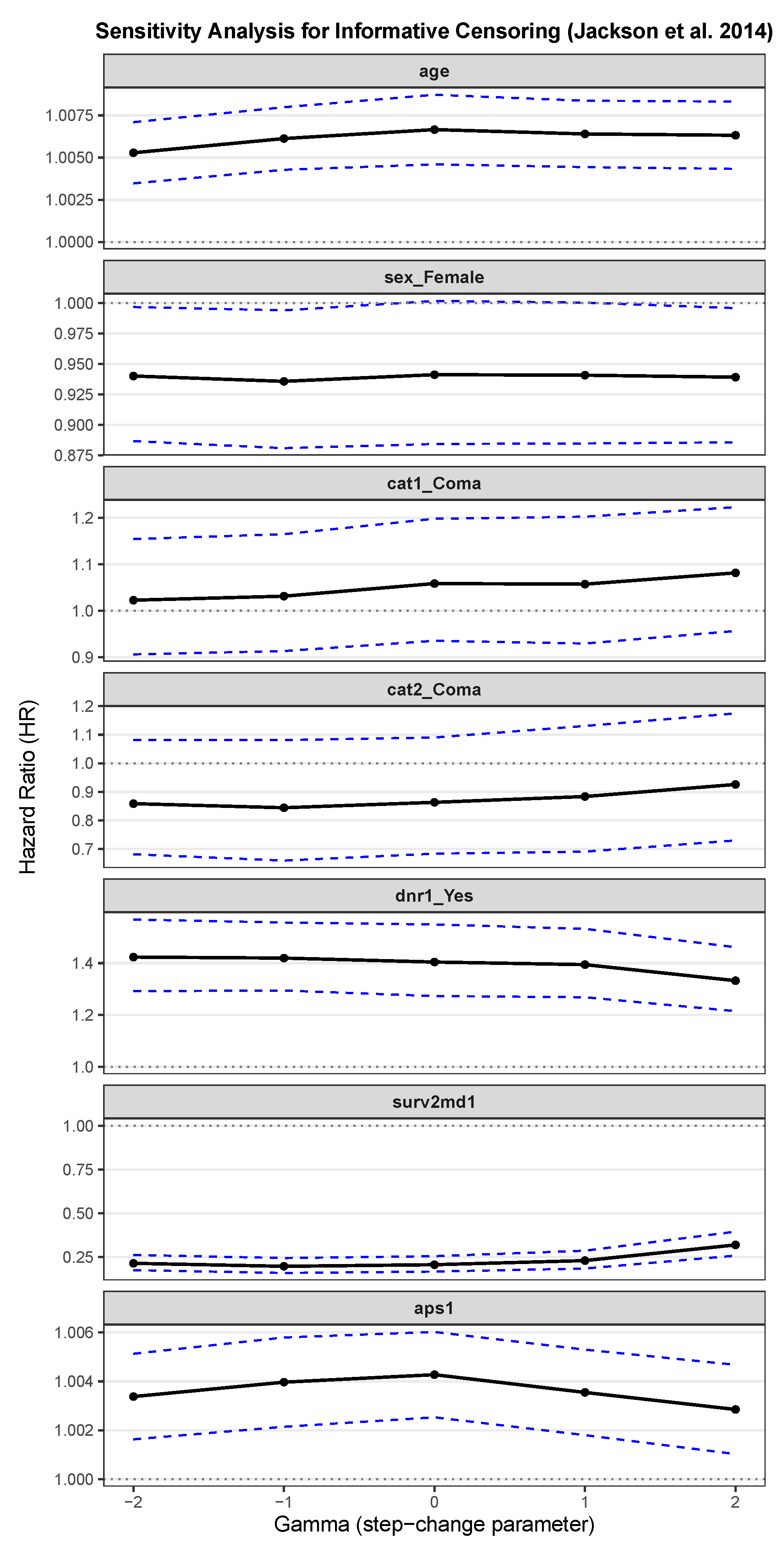
Appendix E. Sensitivity Analysis for Informative Censoring

The informative censoring Assumption 5 is untestable. Given that the dataset contains rich baseline covariates, it is reasonable to assume that censoring is conditionally independent of the event time. Moreover, we conduct a sensitivity analysis based on the imputation of missing failure times using a bootstrap approach. We do not provide a formal test for the independent censoring assumption, but assess the impact of departures from this assumption using a principled multiple imputation approach [41]. This allows us to explore how estimates of the conditional survival function change across a plausible range of values for the sensitivity parameter. Following [41,45], we use Rubin’s rules to present the estimated hazard ratio of several covariates, and 95% confidence intervals, obtained as the estimate plus and minus 1.96 standard errors. The results indicate that the estimation of the conditional survival function is robust regardless of the sensitivity parameter.
Figure A1. Sensitivity analysis for informative censoring assumption [41].
Stats 08 00066 g0a1

References

  1. Cornfield, J.; Haenszel, W.; Hammond, E.C.; Lilienfeld, A.M.; Shimkin, M.B.; Wynder, E.L. Smoking and lung cancer: Recent evidence and a discussion of some questions. J. Natl. Cancer Inst. 1959, 22, 173–203. [Google Scholar] [CrossRef]
  2. Rosenbaum, P.R.; Rubin, D.B. The central role of the propensity score in observational studies for causal effects. Biometrika 1983, 70, 41–55. [Google Scholar] [CrossRef]
  3. Goldberger, A.S. Structural equation methods in the social sciences. Econometrica 1972, 40, 979–1001. [Google Scholar] [CrossRef]
  4. Baker, S.G.; Lindeman, K.S. The paired availability design: A proposal for evaluating epidural analgesia during labor. Stat. Med. 1994, 13, 2269–2278. [Google Scholar] [CrossRef] [PubMed]
  5. Robins, J.M.; Rotnitzky, A.; Zhao, L.P. Estimation of regression coefficients when some regressors are not always observed. J. Am. Stat. Assoc. 1994, 89, 846–866. [Google Scholar] [CrossRef]
  6. Angrist, J.D.; Imbens, G.W.; Rubin, D.B. Identification of causal effects using instrumental variables. J. Am. Stat. Assoc. 1996, 91, 444–455. [Google Scholar] [CrossRef]
  7. Fan, Q.; Zhong, W. Variable selection for structural equation with endogeneity. J. Syst. Sci. Complex. 2018, 31, 787–803. [Google Scholar] [CrossRef]
  8. Miao, W.; Geng, Z.; Tchetgen Tchetgen, E.J. Identifying causal effects with proxy variables of an unmeasured confounder. Biometrika 2018, 105, 987–993. [Google Scholar] [CrossRef]
  9. Tchetgen Tchetgen, E.J.; Ying, A.; Cui, Y.; Shi, X.; Miao, W. An introduction to proximal causal learning. arXiv 2020, arXiv:2009.10982. [Google Scholar]
  10. Cui, Y.; Pu, H.; Shi, X.; Miao, W.; Tchetgen Tchetgen, E. Semiparametric proximal causal inference. J. Am. Stat. Assoc. 2024, 119, 1348–1359. [Google Scholar] [CrossRef]
  11. Qi, Z.; Miao, R.; Zhang, X. Proximal learning for individualized treatment regimes under unmeasured confounding. J. Am. Stat. Assoc. 2024, 119, 915–928. [Google Scholar] [CrossRef]
  12. Shi, X.; Li, K.; Miao, W.; Hu, M.; Tchetgen, E.T. Theory for identification and inference with synthetic controls: A proximal causal inference framework. arXiv 2021, arXiv:2108.13935. [Google Scholar]
  13. Kallus, N.; Mao, X.; Uehara, M. Causal inference under unmeasured confounding with negative controls: A minimax learning approach. arXiv 2021, arXiv:2103.14029. [Google Scholar]
  14. Ghassami, A.; Ying, A.; Shpitser, I.; Tchetgen, E.T. Minimax kernel machine learning for a class of doubly robust functionals with application to proximal causal inference. In Proceedings of the International Conference on Artificial Intelligence and Statistics, PMLR, Virtual, 28–30 March 2022; pp. 7210–7239. [Google Scholar]
  15. Sverdrup, E.; Cui, Y. Proximal causal learning of conditional average treatment effects. In Proceedings of the International Conference on Machine Learning, PMLR, Honolulu, HI, USA, 23–29 July 2023; pp. 33285–33298. [Google Scholar]
  16. Ying, A.; Miao, W.; Shi, X.; Tchetgen Tchetgen, E.J. Proximal causal inference for complex longitudinal studies. J. R. Stat. Soc. Ser. Stat. Methodol. 2023, 85, 684–704. [Google Scholar] [CrossRef]
  17. Dukes, O.; Shpitser, I.; Tchetgen Tchetgen, E.J. Proximal mediation analysis. Biometrika 2023, 110, 973–987. [Google Scholar] [CrossRef]
  18. Shen, T.; Cui, Y. Optimal treatment regimes for proximal causal learning. Adv. Neural Inf. Process. Syst. 2023, 36, 47735–47748. [Google Scholar]
  19. Zhang, J.; Li, W.; Miao, W.; Tchetgen, E.T. Proximal causal inference without uniqueness assumptions. Stat. Probab. Lett. 2023, 198, 109836. [Google Scholar] [CrossRef]
  20. Miao, W.; Shi, X.; Li, Y.; Tchetgen Tchetgen, E.J. A confounding bridge approach for double negative control inference on causal effects. Stat. Theory Relat. Fields 2024, 8, 262–273. [Google Scholar] [CrossRef]
  21. Liu, J.; Park, C.; Li, K.; Tchetgen Tchetgen, E.J. Regression-based proximal causal inference. Am. J. Epidemiol. 2025, 194, 2030–2036. [Google Scholar] [CrossRef]
  22. Bennett, A.; Kallus, N. Proximal reinforcement learning: Efficient off-policy evaluation in partially observed markov decision processes. Oper. Res. 2024, 72, 1071–1086. [Google Scholar] [CrossRef]
  23. Bai, Y.; Cui, Y.; Sun, B. Proximal Inference on Population Intervention Indirect Effect. arXiv 2025, arXiv:2504.11848. [Google Scholar]
  24. Li, Y.; Han, E.; Hu, Y.; Zhou, W.; Qi, Z.; Cui, Y.; Zhu, R. Reinforcement Learning with Continuous Actions Under Unmeasured Confounding. arXiv 2025, arXiv:2505.00304. [Google Scholar]
  25. Ying, A.; Cui, Y.; Tchetgen Tchetgen, E.J. Proximal causal inference for marginal counterfactual survival curves. arXiv 2022, arXiv:2204.13144. [Google Scholar]
  26. Li, K.; Linderman, G.C.; Shi, X.; Tchetgen Tchetgen, E.J. Regression-based proximal causal inference for right-censored time-to-event data. arXiv 2024, arXiv:2409.08924. [Google Scholar] [CrossRef]
  27. Akosile, M.; Zhu, H.; Zhang, S.; Johnson, N.; Lai, D.; Zhu, H. Reassessing the Effectiveness of Right Heart Catheterization (RHC) in the Initial Care of Critically Ill Patients using Targeted Maximum Likelihood Estimation. Int. J. Clin. Biostat. Biom. 2018, 4, 018. [Google Scholar] [CrossRef] [PubMed]
  28. Connors, A.F.; Speroff, T.; Dawson, N.V.; Thomas, C.; Harrell, F.E.; Wagner, D.; Desbiens, N.; Goldman, L.; Wu, A.W.; Califf, R.M.; et al. The effectiveness of right heart catheterization in the initial care of critically III patients. JAMA 1996, 276, 889–897. [Google Scholar] [CrossRef]
  29. Hirano, K.; Imbens, G.W. Estimation of causal effects using propensity score weighting: An application to data on right heart catheterization. Health Serv. Outcomes Res. Methodol. 2001, 2, 259–278. [Google Scholar] [CrossRef]
  30. Diggle, P.; Kenward, M.G. Informative drop-out in longitudinal data analysis. J. R. Stat. Soc. Ser. Appl. Stat. 1994, 43, 49–73. [Google Scholar] [CrossRef]
  31. Scharfstein, D.O.; Robins, J.M. Estimation of the failure time distribution in the presence of informative censoring. Biometrika 2002, 89, 617–634. [Google Scholar] [CrossRef]
  32. Cox, D.R. Regression models and life-tables. J. R. Stat. Soc. Ser. 1972, 34, 187–202. [Google Scholar] [CrossRef]
  33. Klein, J.P.; Moeschberger, M.L. Survival Analysis: Techniques for Censored and Truncated Data; Springer: New York, NY, USA, 2006. [Google Scholar]
  34. Ishwaran, H.; Kogalur, U.B.; Blackstone, E.H.; Lauer, M.S. Random Survival Forests. Ann. Appl. Stat. 2008, 2, 841–860. [Google Scholar] [CrossRef]
  35. Kuroki, M.; Pearl, J. Measurement bias and effect restoration in causal inference. Biometrika 2014, 101, 423–437. [Google Scholar] [CrossRef]
  36. Kompa, B.; Bellamy, D.; Kolokotrones, T.; Beam, A. Deep learning methods for proximal inference via maximum moment restriction. Adv. Neural Inf. Process. Syst. 2022, 35, 11189–11201. [Google Scholar]
  37. Dikkala, N.; Lewis, G.; Mackey, L.; Syrgkanis, V. Minimax estimation of conditional moment models. Adv. Neural Inf. Process. Syst. 2020, 33, 12248–12262. [Google Scholar]
  38. Mastouri, A.; Zhu, Y.; Gultchin, L.; Korba, A.; Silva, R.; Kusner, M.; Gretton, A.; Muandet, K. Proximal causal learning with kernels: Two-stage estimation and moment restriction. In Proceedings of the International Conference on Machine Learning, PMLR, Online, 18–24 July 2021; pp. 7512–7523. [Google Scholar]
  39. Künzel, S.R.; Sekhon, J.S.; Bickel, P.J.; Yu, B. Metalearners for estimating heterogeneous treatment effects using machine learning. Proc. Natl. Acad. Sci. USA 2019, 116, 4156–4165. [Google Scholar] [CrossRef]
  40. Ishwaran, H.; Kogalur, U.B. Random survival forests for R. R News 2007, 7, 25–31. [Google Scholar]
  41. Jackson, D.; White, I.R.; Seaman, S.; Evans, H.; Baisley, K.; Carpenter, J. Relaxing the independent censoring assumption in the Cox proportional hazards model using multiple imputation. Stat. Med. 2014, 33, 4681–4694. [Google Scholar] [CrossRef]
  42. Bang, H.; Robins, J.M. Doubly robust estimation in missing data and causal inference models. Biometrics 2005, 61, 962–973. [Google Scholar] [CrossRef]
  43. Efron, B.; Tibshirani, R.J. An Introduction to the Bootstrap; Chapman & Hall/CRC Press: Philadelphia, PA, USA, 1994. [Google Scholar]
  44. Huang, A.A.; Huang, S.Y. Increasing transparency in machine learning through bootstrap simulation and shapely additive explanations. PLoS ONE 2023, 18, e0281922. [Google Scholar] [CrossRef]
  45. Brooks, B.R.; Berry, J.D.; Ciepielewska, M.; Liu, Y.; Zambrano, G.S.; Zhang, J.; Hagan, M. Intravenous edaravone treatment in ALS and survival: An exploratory, retrospective, administrative claims analysis. eClinicalMedicine 2022, 52, 101590. [Google Scholar] [CrossRef]
Figure 1. The DAG of proximal causal inference for censored data.
Stats 08 00066 g001
Table 1. The simulation results for Case 1, showing absolute bias ( × 10 2 ) and MSE ( × 10 2 ). Lower values of MSE and absolute bias indicate higher precision and accuracy, respectively, with the optimal estimator achieving the smallest values in each row.
ψ ^ DR ψ ^ rf ψ ^ h ψ ^ q ψ ^
Scenario 1bias89.5054.211.174.652.19
MSE82.0533.664.8619.165.77
Scenario 2bias107.7236.2061.294.653.54
MSE127.0319.6270.7419.1620.09
Scenario 3bias99.7145.371.1718.100.23
MSE101.6824.104.8616.084.32
Scenario 4bias134.5625.6737.1244.6246.31
MSE193.5512.4120.8836.1228.55
Table 2. The simulation results for Case 2, showing absolute bias ( × 10 2 ) and MSE ( × 10 2 ). Lower values of MSE and absolute bias indicate higher precision and accuracy, respectively, with the optimal estimator achieving the smallest values in each row.
ψ ^ DR ψ ^ rf ψ ^ h ψ ^ q ψ ^
Scenario 1bias88.2454.871.144.241.77
MSE79.7634.414.4117.174.75
Scenario 2bias107.0937.1459.074.243.47
MSE124.3420.2164.1817.1716.71
Scenario 3bias98.2645.331.1415.720.26
MSE98.7223.964.4114.294.01
Scenario 4bias133.5025.6437.1744.8346.26
MSE189.0912.3020.5534.5127.97
Table 3. The simulation results for Case 3, showing absolute bias ( × 10 2 ) and MSE ( × 10 2 ). Lower values of MSE and absolute bias indicate higher precision and accuracy, respectively, with the optimal estimator achieving the smallest values in each row.
ψ ^ DR ψ ^ rf ψ ^ h ψ ^ q ψ ^
Scenario 1bias42.2733.060.452.850.78
MSE18.4113.881.159.881.23
Scenario 2bias59.1828.2741.692.853.50
MSE42.0411.1236.779.8811.33
Scenario 3bias47.2121.530.4510.730.03
MSE22.897.351.158.721.04
Scenario 4bias78.4617.2627.7233.4334.37
MSE69.175.9912.4721.4416.50
Table 4. Summary statistics of key variables.
VariableMinMaxMedianMean
Outcome / Treatment
A0.0001.0000.0000.381
Y0.0001943.000166.000186.400
Δ 0.0001.0001.0000.649
Treatment proxies (Z)
pafi111.600937.500202.500222.300
paco211.000156.00037.00038.750
Outcome proxies (W)
ph16.5797.7707.4007.388
hema12.00066.19030.00031.870
Control Covariates (X)
age18.040101.85064.05061.380
sex_Female0.0001.0000.0000.443
cat1_Coma0.0001.0000.0000.076
cat2_Coma0.0001.0000.0000.016
dnr1_Yes0.0001.0000.0000.114
surv2md10.0000.9620.6280.593
aps13.000147.00054.00054.670
Table 5. Estimates and 95% CI of treatment effect ( ψ ).
Method ψ ^ 95% CI
UDR−10.169(−22.892, 2.897)
UPCI−7.770(−21.037, 6.388)
DR−20.999(−52.652, 10.698)
PIPW1.389(−58.438, 48.830)
POR−23.447(−54.099, 6.483)
PR−14.781(−41.204, 11.162)
Table 6. Sensitivity analyses under five scenarios of treatment effect ( ψ ).
Method ψ ^ 95% CI
Scenario 1: Z =pafi1, W =hema1
UDR−10.482(−21.813, 2.783)
UPCI−8.124(−23.159, 9.206)
DR−21.442(−52.444, 14.228)
PIPW−7.022(−63.541, 55.390)
POR−24.124(−54.040, 11.595)
PR−18.816(−46.669, 8.624)
Scenario 2: Z =paco21, W =hema1
UDR−10.401(−21.990, 2.051)
UPCI−1.845(−22.985, 21.379)
DR−25.039(−54.214, 6.172)
PIPW−6.482(−95.827, 63.307)
POR−22.117(−52.369, 4.567)
PR−15.049(−48.228, 9.625)
Scenario 3: Z =paco21, W =ph1
UDR−11.337(−23.347, 1.107)
UPCI−21.170(−51.597, 15.252)
DR−27.807(−57.290, 2.800)
PIPW20.098(−54.771, 105.359)
POR−39.741(−65.748, −10.356)
PR−26.708(−65.234, 13.710)
Scenario 4: Z =pafi1, W =ph1
UDR−10.362(−21.593, 1.958)
UPCI−15.077(−29.430, −4.247)
DR−19.277(−48.289, 13.538)
PIPW−6.715(−162.882, 49.252)
POR−28.134(−54.053, 3.064)
PR−19.556(−47.399, 4.201)
Scenario 5: Cox hazard estimation
UDR−10.169(−22.892, 2.897)
UPCI−7.770(−21.037, 6.388)
DR−23.925(−75.414, 23.950)
PIPW2.995(−87.198, 83.571)
POR−23.157(−61.011, 22.261)
PR−15.871(−55.629, 25.948)
Disclaimer/Publisher’s Note: The statements, opinions and data contained in all publications are solely those of the individual author(s) and contributor(s) and not of MDPI and/or the editor(s). MDPI and/or the editor(s) disclaim responsibility for any injury to people or property resulting from any ideas, methods, instructions or products referred to in the content.

