1. Introduction
Since the introduction of the Geometric Brownian Motion (GBM) in one-asset derivative pricing [
1], many theoretical works have tried, with little success, to extend these convenient closed-form solutions to the context of multi-asset derivatives. One key reason is that multidimensional stochastic processes are built from Brownian motions, therefore, even in the favorable scenario of a Gaussian process with non-path-dependent financial derivatives, the price of the product would depend on the multivariate Gaussian distribution. This is, the expected value calculations are doomed to multivariate integrals, solvable numerically via simulations. For more advanced processes, e.g., stochastic covariance model, e.g., see [
2,
3,
4], the price of multi-asset products is rarely analytical, closed-form solutions are available for affine and quadratic models via multivariate Fourier transform methods or simulations (see [
5,
6]). The modelling limitations in multidimensions have also contributed to the absence of path-dependent multi-asset products (see [
7,
8] for rare analytical pricing), in contrast to the popularity of the one-asset path-dependent counterpart, e.g., barrier options, and lookback options; see [
9].
This paper uses standard techniques from Ito’s calculus to design two-dimensional processes (extendable to any dimension), i.e., correlation structures capable of producing analytical solutions for the calculations of specific expectations. These expectations are chosen as the prices of meaningful multi-assets financial derivatives, e.g., spread options and basket options. The perspective introduced here can be extended to not only advanced products like path-dependent derivatives, but also to advanced models on the marginal, like constant elasticity of volatility or stochastic volatility models.
This work benefits from the well-known notion of local variance and local correlation, adapting the latter conveniently. A popular example of a local-variance stochastic process is the constant elasticity of volatility model (CEV), see [
10]. CEV treats volatility as a function of both the current asset level and time while permitting analytical solutions for derivative pricing. On the other hand, the literature on multivariate CEV models (e.g., local-covariance or multivariate local-variance) is scarce and mostly based on numerical approximations (see [
11,
12]).
The literature is scarce on local correlations. The topic has been explored outside of derivative pricing (see [
13,
14] for applications to portfolio optimization), with [
15,
16] describing applications in credit risk. Most existing results are in the direction of our work: derivative pricing. Reference [
17] provides evidence of local correlation under the risk-neutral pricing measure using digital basket options. The author does not aim at analytical solutions, but rather at extracting the dynamics of correlations implied from single-stock options and basket options. Our objective is different as we aim to derive basket option prices analytically from a convenient local correlation structure with GBM dynamics for the stocks. Reference [
18] targets spread options with the idea of combining an endogenous correlation (i.e., driven by the stocks themselves) with exogenous correlation (e.g., Wishart process, non-local) to craft richer and more realistic models. They do not aim for an analytical solution for the financial derivatives. Reference [
19] introduces a calibration scheme for local correlation that ensures a basket’s skew is compatible with the local volatility dynamics of its constituents, but once again, there is no aim at closed-form pricing; see [
20] also for a similar idea. Reference [
21] models the correlation matrix as a linear combination of two constant correlation matrices, i.e., a historical correlation and a worst-case correlation, where the weights are stock-dependent. The authors do not aim at closed-form but rather at fitting existing multi-asset derivatives. Similarly, Reference [
22] studies local correlation models that permit simultaneous calibration to vanilla option prices on all cross-currency pairs, deriving a multi-factor generalisation of the Dupire equation for pricing Best-Of options. Lastly, in the recent work of [
23], the author presents a model with local correlation that explains stylized facts of data, with no intention of producing analytical pricing of multi-asset derivatives.
The paper is organized as follows:
Section 2 presents the general setting as well as examples of derivatives. The main results are described in
Section 3, where the cases of a spread option model and two types of basket option models are defined and studied.
Section 4 discusses the main findings and conclusions.
2. Setting and Methodology
Let all the stochastic processes introduced in this paper be defined on a complete probability space , where is a right-continuous filtration generated by standard Brownian motions , (BMs).
Assume a financial market consisting of 2 risky assets with the following stochastic differential equations (SDE):
where
are scalars capturing the risk-free rate, the volatilities for the assets, and market prices of risks for the first asset and for the intrinsic risk of the second asset (i.e.,
), respectively; while
represents the instantaneous correlation between
and
, hence bounded by −1 and 1. The correlation is assumed to be a function of time and the stocks underlying, which explains the term “local correlation”.
The model above is commonly referred to as the dynamics of stock prices under the historical measure. This dynamic is not helpful for the pricing of financial derivatives, and a change to a risk-neutral measure is required. Let us assume a simple change in measure defined by
, leading to:
where
r is the free rate of interest.
Given the boundness of the process
, there exists a unique strong solution for the SDE under the two measures by simply applying Lipschitz and linear growth conditions (see [
24]).
Let us now assume a contingent claim, i.e., a financial derivative, on the underlying, with payoff
, where
represents the history of the underlying stock,
, from today
t till maturity
T, and
K is a scalar. Examples of this payoff are:
where
and
could be any function of the underlying, for instance
The objective of this paper is to find out the correlation structure on the underlying
and
, such that the process
follows a predetermined stochastic process of the form:
where
could be a function of time and the underlying
that captures the volatility of the option price, and
is a standard Brownian motion. Such a structure for
Y could allow for closed-form pricing of the contingent claim, which is usually unfeasible in multi-asset products. For instance, if
is constant, then we have produced a GBM process for the underlying portfolio in the payoff of the derivative, see the next section for several examples. In this situation, we can use all the tools developed with the Black–Scholes world, not only to price the derivative in closed form, but also to hedge the derivative, i.e., compute Greeks, using the Chain rule. To see this, denote
,
and the price of the derivative, as an expected value under the risk-neutral measure, as
. Then we have
Therefore, , for any variable of interest z.
The next section will show how the idea can be implemented in two cases (Spread and Basket options) and the kind of correlation structure it generates.
3. Results
In this section, we will explore two financial derivatives of interest to practitioners, the spread option and a basket option, where the latter is explored in two cases: two-dimensions and ten-dimensions. In each case, we will derive a convenient correlation such that the payoff follows a Gaussian process.
3.1. Pricing Spread Options
We want to create a correlation structure such that the spread option process
follows the Gaussian process. This is not a classical Ornstein–Uhlenbeck (OU) due to
:
where
and
are scalars to ensure
and
are comparable in value, e.g.,
, and
is assumed deterministic to facilitate the closed-form pricing of options. Other structures would be feasible for our purposes, for instance, CEV models (e.g., [
10]), or stochastic volatility models like [
25].
Applying Ito’s calculus to
:
Assuming a given deterministic
, we get the relation
. Now, we solve for
, leading to:
Note that there is an implicit constraint on
coming from the boundedness of correlations; this constraint is:
Therefore, any proposal for shall stay within those boundaries.
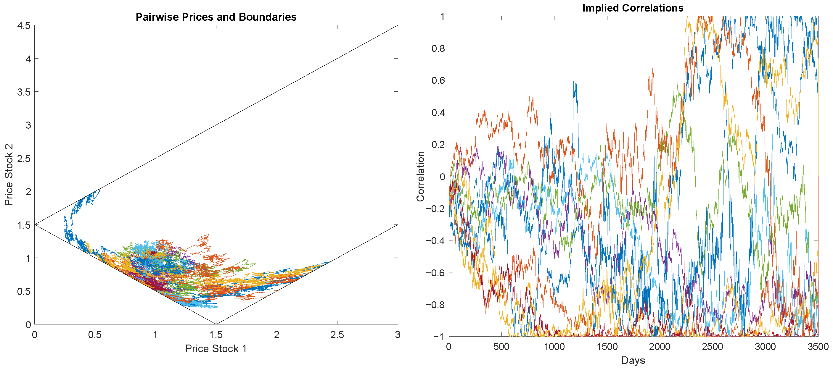
Importantly, and as a key part of the analysis, the constraint on
implies that the joint behaviour of the stocks is limited to a constrained region of the space. To see this for simplicity, let us take
, a constant
, and
, the model forces the stocks to stay within the following bounds:
Figure 1 shows 10 simulated paths of
together with the contained region where the pair is defined. The figure also plots the local correlations implied by the simulated paths. For this simulation, we generate 3500 daily prices with
(i.e., 20% annual volatility),
,
and
. The simulation followed an Euler–Maruyama approximation of the pair of SDE in Equation (
3) with the corresponding constraint on the correlation from Equation (
7).
The marginals of this model are GBM; hence, the pricing of one-asset products remain the same as in the Black–Scholes–Merton (BSM) setting. The benefit of our model is that the price of spread options would be similar to that of BSM formulas, which is (call spread):
where
is the Gaussian cumulative distribution function, and we have used that
is normal with mean
and variance,
The approach described above reveals how a proper correlation structure can lead to well-known processes on a function of the underlying. Other derivatives on can also be priced in closed form thanks to its Gaussian distribution, for instance, put spread options, and products depending on or , e.g., Barrier options, lookback options.
3.2. Pricing 2-Dim Basket Options
We now aim at designing a correlation structure such that
follows the GBM process:
As before, we assume a deterministic
in the relation
, leading to a solution for
as follows:
The model forces the stocks to stay within a viable region; for instance, let us take
. With
, and
, otherwise the region is empty, so we obtain:
Let us denote
, where
; then, we obtain the viable region:
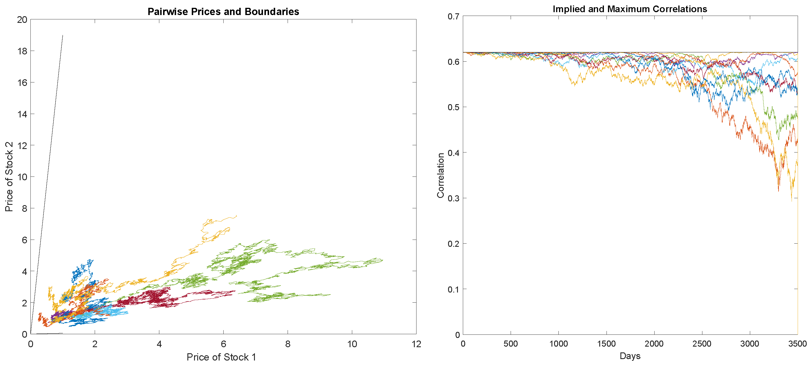
The region leads to an implicit upper bound on the actual correlation, to see this note
where
,
; hence, the maximum correlation is:
.
Figure 2 shows 10 simulated paths of
together with the region where the pair is defined. The figure also plots the local correlations implied by the simulated paths. For this simulation, we generate 3500 daily prices with
(i.e., 20% annual volatility),
,
and
. The simulation followed an Euler–Maruyama approximation of the pair of SDE in Equations (
3) with the corresponding constraint on the correlation from Equation (
9).
The margin of this model is GBM, with all its benefits for pricing one-asset products. On the other hand, the price of basket options would be similar to BSM formulas. For simplicity, let us take
:
where
,
.
As before, other derivatives on can also be priced in closed form thanks to the GBM connection, for instance, put basket options, and products depending on or , e.g., Barrier options, lookback options.
3.3. Pricing n-Dim Basket Options
For more than two assets, a single local correlation construction can be constructed within a GBM in multidimensions as follows:
where
stands for the volatility of the asset
, and
,
are independent Brownian motions. If working with a basket option,
, and a GBM process for
, then the correlation must have the form:
To see this, let
follow the GBM process:
Applying Ito’s to
:
As before, we assume a deterministic
in the relation:
leading to the given solution for
.
The model forces the stocks to stay within a viable region; for instance, let us take
,
. The boundedness of
by 0 and 1, together with
leads to:
which in particular implies
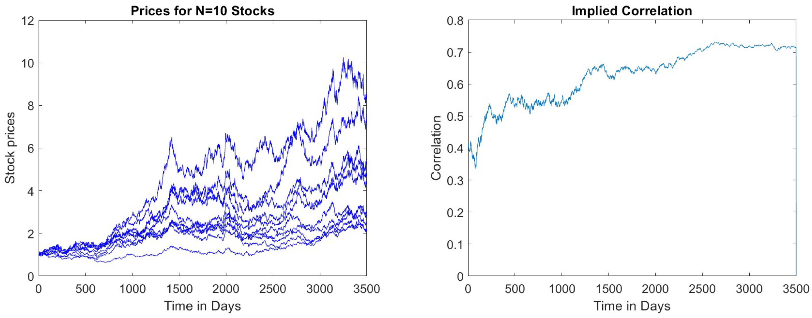
.
Figure 3 shows a simulated path of the vector
, where
. The figure also plots the local correlation implied by the simulated path. As before, we generate 3500 daily prices with
(i.e., 20% annual volatility),
,
and
. We followed a Euler–Maruyama approximation of the system of SDE in Equation (
3).
As examined before, the marginal of this model is GBM with all its benefits for pricing one-asset products. And the price of the basket options would be similar to BSM formulas. For simplicity, let us take
:
where
,
.
Needless to say, our proposal above is just an example; we can construct many others. For instance, more than a one-factor local correlation is also viable and worth exploring. This could be handled, for example, with a model with
n correlations
, where for each
, we have that
is a GBM with volatility
, and
. Such a setting would define correlations sequentially, with GBM for the underlying stocks leading to:
4. Discussion
As highlighted in the introduction, this paper provides a methodology to define multivariate processes with convenient marginal and dependence structure in continuous-time. For simplicity of presentation, we focused on two dimensions (two assets) with GBM marginals and two special derivatives, basket and spread options, where the contingent claims are modelled as either a GBM or an OU with time-dependent volatilities.
The results obtained for the two considered cases are quite promising and far-reaching. The new models, especially the new correlation structures, have opened the door to analytical solutions for multidimensional derivatives. Pricing high-dimensional products has almost exclusively been the realm of Monte Carlo simulations, which makes the pricing quite time-consuming and potentially inaccurate, especially in high dimensions. Needless to say, closed-form pricing, like the famous Black–Scholes formulas, has been a favourite of practitioners for decades due to their practically instantaneous pricing. Fast pricing methods allow institutions to evaluate portfolios and positions in a timely manner, serving internal and regulatory purposes. Analytical expressions are even used as quick approximations to more complex representations; it is in this spirit that our methodology can benefit practitioners.
Although our approach is not designed, in principle, to capture the joint behaviour of assets under specific market conditions, the method has a hidden degree of freedom. It allows users to attach well-known stochastic processes to the payoff of a derivative, creating a degree of freedom to capture desired market conditions or joint behaviours. This additional flexibility also implies multiple feasible correlation structures in the modelling of real multivariate data. Nonetheless, our methodology brings a level of realism to the behaviour of correlations, making them stochastic and related to the underlying assets while generating reasonable regions for joint stock price movements.
The concept presented here could be extended in many directions. First, we could have assumed a contingent claims processes (
) that follow CEV or stochastic volatility (SV) models; for instance, models for
, like in [
25,
26], enrich the dynamics of the implied correlation structure. A CEV model looks like:
where
could be interpreted as the elasticity of the volatility of the option price. While an SV model would be:
where
basically describes the stochastic variance of the option price driven by a Brownian motion
, potentially correlated to
, with its corresponding CIR parameters
, and
.
Nonetheless, readers should be aware of the potential pitfalls of such extensions, which should be treated carefully. For instance, there are complexities in pricing options under these more advanced models, i.e., the need for the Fourier transform and confluent hypergeometric functions as part of the pricing formulas. Second, proper uniqueness and existence of a solution for the resulting SDE of the process can not be taken for granted; so far, we managed to deliver these good properties assuming a Gaussian process for and GBM for the assets, which is no longer the case in this most general setting.
We could also consider other types of options, in particular, barrier and path-dependent products, which would be solvable even for the SV case mentioned above (see [
27] for closed-form solutions).
Higher dimensions, i.e., more than two assets, are also feasible, particularly with a single local correlation using a one-factor construction as in the previous section.
With
assets, we enter into more complex derivatives like the world of mountain range products, rainbow options, collateralized debt obligations, collateralized fund obligations and structured products (see [
28,
29,
30,
31,
32,
33]), which would likely be solvable in closed-form thanks to the convenient correlation structure.
Lastly, given the same objective of closed-form solutions for pre-specified financial derivatives, the previous examples of extensions are by no means exhaustive. We could have assumed generic Ito processes or Fractional Brownian driving the underlying assets, leading to local correlations, or even Levy processes for the underlyings, creating richer local dependence rather than correlation structures. These ideas shall be explored in future research as a way to tackle the complexities of dependence structures in the world of financial assets.


