The Detection Method of the Tobit Model in a Dataset

Abstract

This article proposes an extension of detection methods for the Tobit model by generalizing existing approaches from cases with known parameters to more realistic scenarios where the parameters are unknown. The main objective is to develop detection procedures that account for parameter uncertainty and to analyze how this uncertainty affects the estimation process and the overall accuracy of the model. The methodology relies on maximum likelihood estimation, applied to datasets generated under different configurations of the Tobit model. A series of Monte Carlo simulations is conducted to evaluate the performance of the proposed methods. The results provide insights into the robustness of the detection procedures under varying assumptions. The study concludes with practical recommendations for improving the application of the Tobit model in fields such as econometrics, health economics, and environmental studies.

1. Introduction

The Tobit model was introduced by James Tobin [1] in his seminal work on consumer behavior, specifically analyzing expenditures on durable goods while accounting for the fact that such expenditures cannot fall below zero. This gave rise to the concept of limited dependent variable models, where the dependent variable is subject to censoring or truncation. The term Tobit model—coined by Goldberger [2]—has since become a cornerstone in econometrics, particularly for modeling situations in which the outcome variable has a restricted domain.

In the classical Tobit model (Type I), the latent variable follows a normal distribution, and observed values are censored at a certain threshold—typically zero. Amemiya [3] categorized several variations of the Tobit model, including Types II to V, which handle selection bias, multiple equations, and other data complications.

Tobit models have been extensively used not only in economics but also in other fields such as biometrics, engineering, and environmental sciences. In  biometrics, for instance, they help model survival times with censoring; in engineering, they apply to reliability analysis.

However, a key limitation of the standard Tobit framework lies in its reliance on the normality assumption for the error terms. In practice, this assumption is often violated. Several studies have extended the Tobit model to incorporate non-normal error distributions, including symmetric alternatives (e.g., Student’s t, logistic) and asymmetric distributions (e.g., skew-normal, generalized lambda). Works by Powell (1986) [4], Arabmazar and Schmidt (1981) [5], and  others have explored semi-parametric and non-parametric Tobit models to improve robustness when the distribution of errors is unknown or misspecified. Robust estimation approaches, such as the Student t-based M-estimator proposed by Lucas [6], have been developed to address sensitivity to outliers and heavy-tailed distributions.

More recently, efforts have been made to adapt Tobit-type models to accommodate log-symmetric and asymmetric distributions, particularly in the presence of censored data. Vanegas and Paula [7,8,9,10,11] have developed a comprehensive statistical framework for log-symmetric regression models, addressing their properties [7], applications to censored data with non-informative censoring [10], and implementation through a recent R package for semi-parametric estimation [11]. Saulo et al. [12,13] extended this work to asymmetric models and further applied them in censored settings. These approaches offer improved flexibility and robustness when classical normality-based assumptions are not valid. Medeiros and Ferrari [14] further contributed to this line by offering inference techniques for symmetric and log-symmetric linear regression models, suitable for contexts involving multiplicative and non-normal error structures.

In this paper, we contribute to this line of research by exploring detection methods for the Tobit model under parameter uncertainty. While prior studies have focused on the case where model parameters are known [15], we extend this analysis to more realistic situations in which these parameters must be estimated. The goal is to assess how uncertainty in parameter estimation influences the reliability of Tobit model detection.

The remainder of this paper is structured as follows. Section 1 discusses parametric estimation techniques for the Tobit model, including least squares and maximum likelihood estimators. Section 2 addresses statistical procedures for detecting the presence of a Tobit structure in the data. In Section 3, we use Monte Carlo simulations to evaluate the performance of these procedures under various conditions. The final section provides conclusions and suggestions for future research.

2. Parametric Estimation

In this section, we present the parametric estimators associated with the Type 1 Tobit model, namely the least squares estimator and the maximum likelihood estimator.

Definition 1.

The simple Tobit model (Type 1) is defined as follows:

$$y_i=\left\{\begin{array}{cc}{y}_i^{*}\hfill & if{y}_i^{*}>0,\hfill \\ 0\hfill & if{y}_i^{*}\le 0,\hfill \end{array}\right.$$

(1)

where

$$y_i^{*}=x_i\beta +{\epsilon }_i,i=1,\dots ,N,$$

with $y_i$ denoting the observable variable corresponding to the latent variable $y_i^{*}$, $x_i=(x_i^1,\dots ,x_i^K)$ representing the vector of observable variables, ${\beta }^{\prime }=({\beta }_1,\dots ,{\beta }_K)\in {\mathbb{R}}^K$ being the vector of unknown parameters, and $\left({\epsilon }_i\right)$ are the independent and identically distributed errors terms, assumed to follow a normal distribution $N(0,{\sigma }^2)$.

2.1. Example

Let  $y_i$ be the number of purchases of durable goods. If a person’s salary is greater than a certain threshold C, the amount spent is proportional to the salary. If the person’s salary is below this threshold, there are no purchases of durable goods.

Remark 1.

In the case of the previous example, the model is written as follows:

$$y_i=\left\{\begin{array}{c}{y}_i^{*}if{y}_i^{*}>C\\ cif{y}_i^{*}\le C.\end{array}\right.$$

To find the model (2.1), we translate the variable $y_i^{*}$ by an amount $-C$.

2.2. Least Squares Estimator

2.2.1. First Case: The Exogenous Variables $\left(x_i\right)$ Are Deterministic

The LS estimator, applied to all N pairs of observations $(y_i,x_i)$, is defined as follows:

$${\widehat{\beta }}_{LS}={\left({\displaystyle \sum _{i=1}^{i=N}}{x}_i^{\prime }{x}_i\right)}^{-1}\sum _{i=1}^{i=N}{x}_i^{\prime }{y}_i.$$

Even though it is easy and extremely prevalent, the LS estimator is inconsistent in the context of censored models such as the Tobit model [7]. This inconsistency stems from its failure to account for the censoring mechanism, typically at zero. This omission leads to an asymptotic and systematic downward bias in the estimated regression coefficients. Specifically, as shown by Amemiya [3] and Greene [16] the bias arises because OLS underestimates the effect of the explanatory variables in absolute terms, especially when a large proportion of observations are censored. While in very simple settings (e.g., univariate models with normal errors and known thresholds), a closed-form expression of this asymptotic bias can be derived [17] (see Maddala1983, Chapter 9), in general, the expression becomes analytically intractable due to the dependency on the joint distribution of the latent dependent variable and the covariates. In light of this, Proposition 2 in our paper formally establishes the asymptotic inconsistency of the LS estimator in the censored framework. We clarify that the “bias” we refer to throughout this section is indeed asymptotic in nature.

2.2.2. Second Case: $x_i$ Are Random Variables

In the case where the exogenous variables $x_i$ are random, Goldberger [18] analyzed this case by introducing a constant term to the regression equation. The Tobit model can therefore be expressed as follows:

$$y_i=\left\{\begin{array}{c}{y}_i^{*}if{y}_i^{*}>0\\ 0if{y}_i^{*}\le 0\end{array}\right.$$

(2)

with

$$y_i^{*}=\alpha +x_i\beta +{\epsilon }_i,i=1,\dots ,N,$$

where $x_i=(x_i^1,\dots ,x_i^K)$ is a vector of random normal distribution $N(0,\Omega ),$ with $\Omega$ being a positive definite $K\times K$ matrix. The unknown parameters are as follows:

$${\beta }^{\prime }=({\beta }_1,\dots ,{\beta }_K)\in {\mathbf{R}}^K,\alpha \in \mathbf{R}$$

(3)

This structure recognizes the stochastic nature of explanatory variables in empirical economic data and is a major advance over deterministic models. Goldberger’s work paved the way for a more nuanced understanding of censored data models and established the basis for more robust estimation methods that are aware of the underlying data-generating process.

Fundamental assumption (FH)

We assume that the variables $\left(x_i\right)$ follow a multivariate normal distribution: $N(0,\mathrm{\Omega }),$ with the additional condition that

$$cov({\epsilon }_i,x_i^k)=0,forallk=1,\dots ,K.$$

Proposition 1

(Greene [16]). Under the assumption (FH), the least squares (LS) estimator is computed using all observations $(x_i,y_i)$, which satisfies ${\widehat{\beta }}_{LS}\to \beta \times \mathrm{\Phi }\left({\displaystyle \frac{\alpha }{{\sigma }_y}}\right)$, in probability, when $N\to \infty$, where ${\sigma }_y^2={\sigma }^2+{\beta }^{\prime }\mathrm{\Omega }\beta$. Moreover, under the assumption (FH), the estimator defined by ${\widehat{\beta }}_{LSC}=(N/N_1)\times {\widehat{\beta }}_{LS},$ where $N_1$ is the number of observations for which $y_i^{*}>0$, is a consistent estimator of β: ${\widehat{\beta }}_{LSC}⟶\beta ,inprobability,whenN⟶\infty$.

2.3. Maximum Likelihood Estimator

For several decades, simpler estimation procedures—such as Heckman’s two-step method [19]—were used because they were less computationally intensive. These processes had workable solutions when computational capacity was not as great.

However, with the advent of computers that can efficiently solve complex optimization problems, the Maximum Likelihood Estimator (MLE) has found extensive application. The MLE approach uses the whole probabilistic model structure and tends to yield estimators with good asymptotic properties.

Through the use of the reparametrization constructed by Olsen [20], the log-likelihood function of the Tobit model can be written as:

$$\begin{array}{ccc}\hfill \sum _{i:y_i>0}logL(y,\theta ,h)& =& \sum _{i:y_i=0}log(1-\mathrm{\Phi }\left(x_i\theta \right))-1/2\sum _{i:y_i>0}{(h{y}_i-x_i)}^2+N_{1}log\left(h\right)\hfill \end{array}$$

where $N_1$ is the number of observations for which $y_i>0$. The LM estimator $\widehat{\gamma }={(\widehat{{\theta }^{\prime }},\widehat{h})}^{\prime }$ of $\gamma$ is the solution to the following problem:

$$\widehat{\gamma }=arg\underset{\gamma }{max}logL(y,\gamma )=arg\underset{(\theta ,h)}{max}logL(y,\theta ,h).$$

Amemiya [3] proved that the maximum likelihood estimator $\widehat{\beta }=\widehat{\theta }/\widehat{h}$ and $\widehat{\sigma }=1/\widehat{h}$ are strongly consistent and asymptotically normal.

3. Detection of Tobit Model

3.1. Reminder on Tobit Model Detection (When Parameters Are Known)

3.1.1. Problem Setup

In this section, we give statistical tools for the detection of a Tobit model to from observations of a sample.

Let $\xi$ be a sample of points $(x_i,y_i)$ for $i=1,\dots ,n$. The objective is to determine if there exists a latent variable $y^{*}$ satisfying:

$$y^{*}=x_i\beta +\alpha +{\epsilon }_i$$

where:

• with $\alpha ,\beta ,{\sigma }^2$ known
• $x_i$ are the explanatory variables,
• $\beta$ is the parameter vector,
• $\alpha$ is a constant,
• ${\epsilon }_i$ are errors that are independent and identically distributed (i.i.d.) following a normal distribution $\mathcal{N}(0,{\sigma }^2)$,
• $y_i$ is observed as $y_i=max(0,y_i^{*})$ (the variable is censored at zero).

3.1.2. Note

Without loss of generality, Proposition 2 remains valid if we replace $y_i=max(0,y_i^{*})$ with $y_i=max(k,y_i^{*})$, where k is a given constant.

Proposition 2

(Conditions for the detection of the Tobit model [15]). The problem admits a solution if the following conditions are satisfied:

1. 

Condition 1 (For $y_i>0$): For all $i\in \{1,\dots ,n\}$ such that $y_i>0$, the  error ${\epsilon }_i$ is calculated as follows:

$${\epsilon }_i=y_i-x_i\beta -\alpha$$

This means that for observations where $y_i$ is strictly positive, the error ${\epsilon }_i$ is simply the difference between the observed $y_i$ and the predicted value $x_i\beta +\alpha$.

2. 

Condition 2 (For $y_i=0$): For each $i\in \{1,\dots ,n\}$ such that $y_i=0$, there exists an error ${\epsilon }_i$ such that the latent variable $y_i^{*}=x_i\beta +\alpha +{\epsilon }_i$ is negative, i.e.,  $y_i^{*}<0$.

3. 

Condition 3 (Distribution of Errors): The latent variable $y_i^{*}$ follows a standard normal distribution, i.e.,

$${\displaystyle \frac{y_i^{*}-x_i\beta -\alpha }{\sigma }}\sim \mathcal{N}(0,1)$$

for all $i=1,\dots ,n$. This implies that the errors ${\epsilon }_i$ are normally distributed with variance ${\sigma }^2$.

3.1.3. Summary of the Approach

The underlying idea of the Tobit model is that each observation is associated with a latent (unobserved) variable $y_i^{*}$ that follows a linear model:

$$y_i^{*}=x_i^{\top }\beta +\alpha +{\epsilon }_i,{\epsilon }_i\sim \mathcal{N}(0,{\sigma }^2).$$

However, the observed outcome $y_i$ is left-censored at c:

$$y_i=max(c,y_i^{*}).$$

• For observations where $y_i>c$ (uncensored), we have $y_i=y_i^{*}$, and the residual can be directly estimated as follows:

  $${\widehat{\epsilon }}_i=y_i-{\widehat{y}}_i=y_i-x_i^{\top }\widehat{\beta }-\widehat{\alpha }.$$
• For observations where $y_i=c$ (censored), the latent value $y_i^{*}$ is unobserved and satisfies the following:

  $$y_i^{*}\le c\Rightarrow {\epsilon }_i\le -x_i^{\top }\beta -\alpha .$$
  In this case, ${\epsilon }_i$ is not point-identifiable but lies in the truncated interval $(-\infty ,-x_i^{\top }\beta -\alpha ]$. To approximate the latent value $y_i^{*}$ and the residual, we proceed as follows (see Section 3.2):

  –

  We use the Tobit estimates $\widehat{\beta }$ and $\widehat{\alpha }$ to compute the predicted value:

  $${\widehat{y}}_i=x_i^{\top }\widehat{\beta }+\widehat{\alpha }.$$

  –

  We simulate ${\epsilon }_i\sim \mathcal{N}(0,{\widehat{\sigma }}^2)$ and construct:

  $$y_i^{*}={\widehat{y}}_i+{\epsilon }_i,$$

  accepting only those simulations where $y_i^{*}\le c$. This guarantees consistency with the censoring.

  –

  The residual is then approximated as follows:

  $${\widehat{\epsilon }}_i=y_i^{*}-{\widehat{y}}_i.$$

This procedure enables consistent residual estimation for both censored and uncensored observations, despite the unobservability of $y_i^{*}$ in the former case.

3.2. Tobit Model Detection (When Parameters Are Unknown)

We extend the detection framework for the Tobit model from the case where parameters are known to the more realistic scenario in which the parameters must be estimated. In this context, it is important to highlight the fundamental properties of the maximum likelihood estimator (MLE), which justify its use for such an extension. Specifically, the MLE is consistent—meaning it converges to the true parameter values as the sample size increases—and asymptotically normal, implying that its sampling distribution approaches a normal distribution centered on the true parameters, with an estimable variance, for large sample sizes.

These properties of the MLE provide a solid foundation for constructing a robust framework for estimation and model detection under parameter uncertainty. The theoretical Proposition 2 used in the known-parameter case remains applicable; the key difference is that the detection procedure now relies on estimated parameter values rather than known ones, under the same model assumptions.

3.2.1. Note

To determine whether a Tobit model is suitable for a given dataset, two complementary approaches can be employed:

3.2.2. Method Based on the Application of Proposition 2

This approach [15] involves evaluating whether the data satisfy the fundamental assumptions that justify the use of a Tobit model. Specifically, it examines:

• The presence of censoring (typically left-censoring at zero or another threshold),
• A linear relationship between the (latent) dependent variable and the explanatory variables,
• The nature of the error distribution and its compatibility with Tobit assumptions.

These checks serve as a preliminary validation step before estimation, helping to confirm whether the Tobit model is conceptually appropriate for the context.

3.2.3. Based on Fitting the Data with the Tobit Model

The second approach involves estimating the Tobit model using maximum likelihood methods implemented in statistical software (e.g., Stata, R-4.5.1, Python 3.12). Once the parameters are estimated, model adequacy is evaluated based on:

• The statistical significance of estimated coefficients,
• Goodness-of-fit metrics such as the log-likelihood or pseudo-$R^2$,
• Diagnostic tools, including residual analysis and graphical comparisons of observed versus predicted values.

This empirical method not only assesses model fit but also helps determine whether the Tobit specification captures the key features of the data.

By combining these two approaches—theoretical validation and empirical assessment— researchers can more confidently determine whether the Tobit model is appropriate for their specific application. These detection methods are particularly relevant in fields such as labor economics, consumer behavior analysis, healthcare utilization studies, and environmental modeling, where censored outcomes frequently arise.

4. Application

Let a sample $\xi$ of points $(x_i,y_i)\in E$, with:

$$E=\{(x_i,y_i)\mid x_i\in X,y_i\in Y\}$$

$$X=\mathrm{seq}(0.1,7.5)$$

$$\begin{array}{cc}\hfill Y=\{& 4.000000,4.000000,4.000000,4.000000,4.000000,4.000000,4.000000,4.000000,\hfill \\ \hfill & 4.000000,4.000000,5.675606,4.000000,4.000000,4.730979,4.061686,5.026789,\hfill \\ \hfill & 4.451797,4.541571,4.890612,5.412781,4.589914,4.744637,5.415221,5.971301,\hfill \\ \hfill & 5.682624,6.516985,5.298265,5.169042,8.692011,7.397877,6.802972,7.120042,\hfill \\ \hfill & 8.385119,7.589679,8.192115,7.935274,7.898609,9.202190,8.941495,10.301813,\hfill \\ \hfill & 8.074603,9.264693,9.391011,8.725138,10.997859,10.092600,9.014442,10.007859,\hfill \\ \hfill & 9.694666,12.039089,13.742904,10.726284,11.507770,12.079735,14.708959,9.870997,\hfill \\ \hfill & 11.886044,11.397205,12.572375,12.724101,12.470191,15.234156,13.857065,16.193585,\hfill \\ \hfill & 14.823617,12.934688,13.646509,14.873038,14.222101,15.354290,15.932573,15.821122,\hfill \\ \hfill & 15.465387,15.156461,14.710679\}\hfill \end{array}$$

Using R software, we obtained the estimated values of the parameters for the Tobit model.

We then generated the observed values $y_i$, subject to the left-censoring condition:

$$y_i=max(4,z_i)$$

This implies that if $z_i>4$, the observation is uncensored and $y_i=z_i$. If $z_i\le 4$, the observation is censored, and we simulate the latent variable $y_i^{*}$ using:

$$y_i^{*}={\widehat{y}}_i+{\epsilon }_i,$$

where ${\widehat{y}}_i=\widehat{\beta }{x}_i+\widehat{\alpha }$, and ${\epsilon }_i\sim \mathcal{N}(0,1)$. We accept only those simulated values such that $y_i^{*}\le 4$, in accordance with the censoring rule. This process is repeated until the condition is satisfied. The accuracy of this approach is verified using a scatter plot.

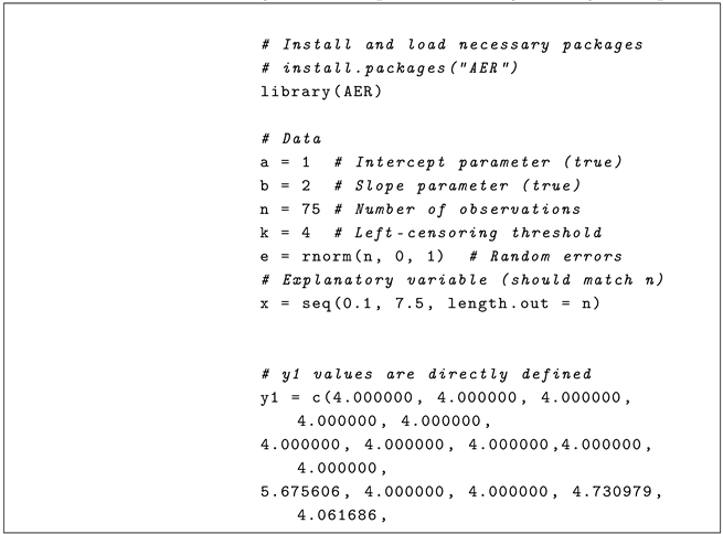
To simulate data consistent with a Tobit model, we define the latent variable as:

$$z_i=2x_i+1+{\epsilon }_i,$$

where $x_i=\mathtt{seq}(0.1,7.5,\mathtt{length}.\mathtt{out}=75)$ and ${\epsilon }_i\sim \mathcal{N}(0,1)$ is generated using rnorm(75, 0, 1) in R. The observed variable is then computed as $y_i=max(4,z_i)$.

This construction corresponds to a Tobit model with left-censoring at 4. The  true parameter values used for simulation are $\beta =2$, $\alpha =1$, and  ${\sigma }^2=1$. These values were intentionally chosen to produce realistic yet controlled data, allowing us to assess the consistency and correctness of the estimation procedure.

To reconstruct the latent variable set $E^{\prime }={\left\{y_i^{*}\right\}}_{i=1}^{75}$, we apply the following logic:

• If $y_i>4$, then $y_i^{*}=y_i$ (observation is uncensored).
• If $y_i=4$, then $y_i^{*}=\widehat{\beta }{x}_i+\widehat{\alpha }+{\epsilon }_i$, accepting only those simulations where $y_i^{*}\le 4$ (observation is censored). This process is repeated if necessary.

The final set $E^{\prime }$ thus consists of:

• The actual observed values for uncensored data.
• Simulated latent values for censored observations.

We then compute the residuals:

$${\widehat{\epsilon }}_i=y_i^{*}-(\widehat{\beta }{x}_i+\widehat{\alpha }),$$

to evaluate whether their empirical distribution approximates the standard normal distribution $\mathcal{N}(0,1)$, as required by the theoretical assumptions of the Tobit model.

The R code used to estimate the Tobit model parameters is provided in Appendix A and Appendix B.

The estimation output gives the following parameter values:

• $\widehat{\alpha }=1.093579$
• $\widehat{\beta }=1.981041$
• ${\widehat{\sigma }}^2=1$

Thus, we can obtain all the values of $y^{*}$ belonging to a set E’, where:

$$\begin{array}{cc}\hfill E^{\prime }=\{& 2.1037102,1.7954352,2.0835080,2.2707734,2.2789433,2.5608576,0.9436878,\hfill \\ \hfill & 1.8313552,3.4204762,2.6894289,5.6756060,1.3519320,2.5457927,4.7309790,\hfill \\ \hfill & 4.0616860,5.0267890,4.4517970,4.5415710,4.8906120,5.4127810,4.5899140,\hfill \\ \hfill & 4.7446370,5.4152210,5.9713010,5.6826240,6.5169850,5.2982650,5.1690420,\hfill \\ \hfill & 8.6920110,7.3978770,6.8029720,7.1200420,8.3851190,7.5896790,8.1921150,\hfill \\ \hfill & 7.9352740,7.8986090,9.2021900,8.9414950,10.3018130,8.0746030,9.2646930,\hfill \\ \hfill & 9.3910110,8.7251380,10.9978590,10.0926000,9.0144420,10.0078590,9.6946660,\hfill \\ \hfill & 12.0390890,13.7429040,10.7262840,11.5077700,12.0797350,14.7089590,9.8709970,\hfill \\ \hfill & 11.8860440,11.3972050,12.5723750,12.7241010,12.4701910,15.2341560,13.8570650,\hfill \\ \hfill & 16.1935850,14.8236170,12.9346880,13.6465090,14.8730380,14.2221010,15.3542900,\hfill \\ \hfill & 15.9325730,15.8211220,15.4653870,15.1564610,14.7106790\}\hfill \end{array}$$

All that remains is to verify the conditions of Proposition 2. We define $\epsilon =y^{*}-b_{\mathrm{predict}}·x-a_{\mathrm{predict}}$. Thus, the first condition is satisfied (because if $y_1>4$, then $y^{*}=y_1$, and we have

$${\epsilon }_i=y_{1i}-b_{\mathrm{predict}}·x-a_{\mathrm{predict}}$$

The second condition is satisfied by the construction of ${\epsilon }_i$.

It remains to verify the third condition, which is that

$${\displaystyle \frac{y_i^{*}-b_{\mathrm{predict}}·x_i-a_{\mathrm{predict}}}{{\sigma }_{\mathrm{predict}}}}$$

follows a standard normal distribution (mean zero and variance one). To achieve this, we perform a Kolmogorov–Smirnov test (see Appendix B) for the test code using the R software (version 4.2.1)). The output of the code provides the following results:

• Null hypothesis (${\mathit{H}}_{\mathbf{0}}$): The data $\epsilon$ follow a normal distribution.
• Decision based on the $\mathit{p}$-value:
  • If $p>0.05$, we fail to reject the null hypothesis. The data are compatible with a normal distribution.
  • If $p\le 0.05$, we reject the null hypothesis. The  data likely do not follow a normal distribution.

In this case: The p-value is p = 0.3816986, which is greater than 0.05. Therefore, we fail to reject the null hypothesis. The residuals e can be considered as following a normal distribution. However, it is important to note that failing to reject the null hypothesis does not prove normality; it only suggests that the normality assumption is plausible given the data. For additional insight, a graphical inspection (e.g., Q-Q plot or histogram) may also be considered. The output of the code (Appendix B) shows: Mean of residuals: −0.06540354 −0.06540354 and Standard deviation of residuals: 1.014941 1.014941.

Conclusion: The three conditions of Proposition 2 are satisfied, hence the existence of $y_i^{*}$ such that $y_{1i}=max(4,y_i^{*})$ for all $i=1,2,\dots ,75$.

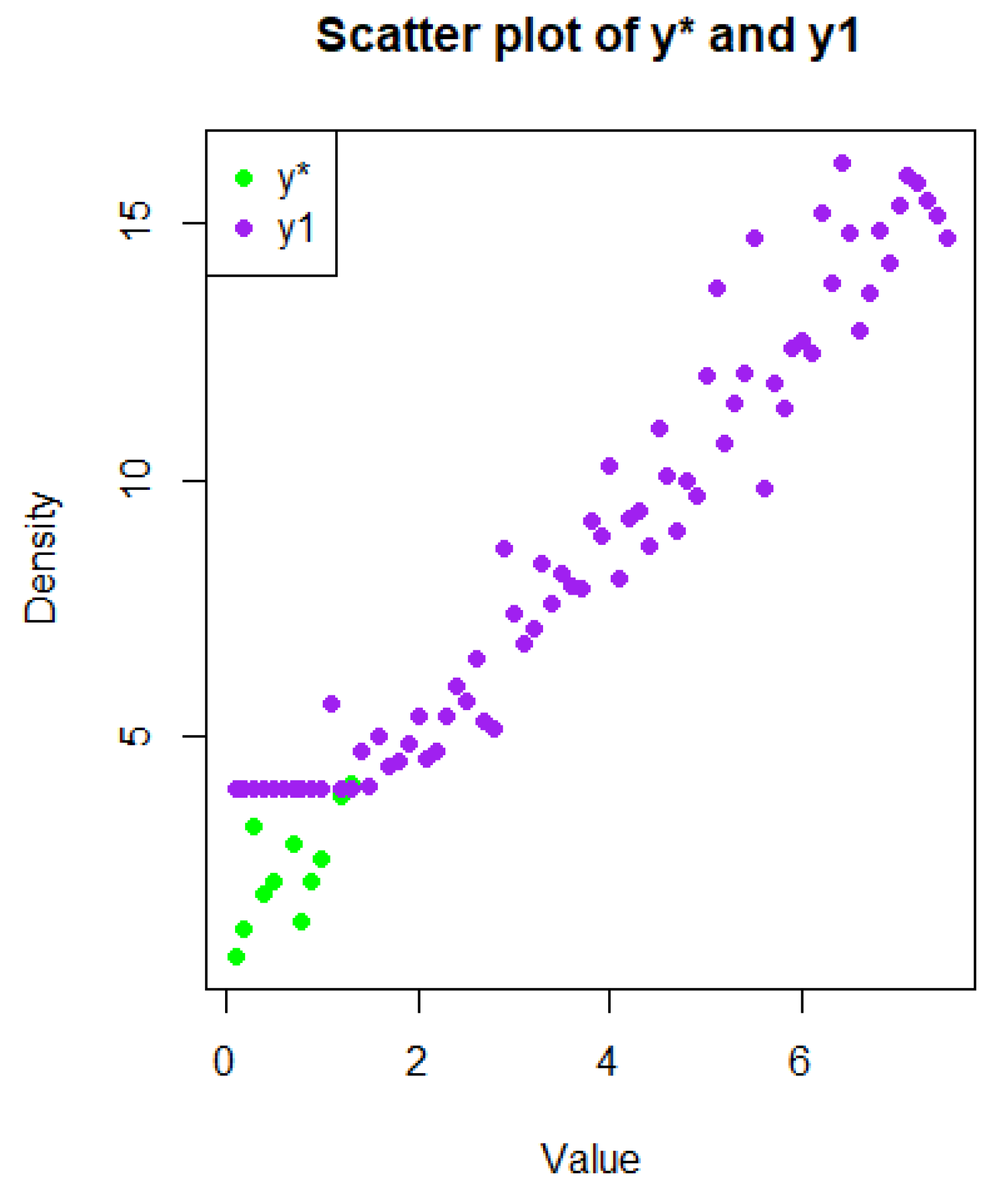
5. Visualization

The Figure 1 below represents the visualization:

6. Project Objective

This mini-project (Appendix B) aims to illustrate the detection and validation of a Tobit model in a simulated context. The goal is to demonstrate, using an artificially generated dataset with censored values, how to identify the relevance of a Tobit model, estimate its parameters, and analyze its performance.

6.1. Background and Justification

The Tobit model is used when the dependent variable is censored, meaning it is truncated at a certain threshold. This situation commonly arises in economics, sociology, or engineering. In this project, we simulate a case of left-censoring at a fixed threshold $k=4$, which justifies the use of a Tobit model.

6.2. Methodology

6.2.1. Data Generation

• Number of observations: $n=75$
• Latent model:

  $$y_i^{*}=a+b{x}_i+{\epsilon }_i,{\epsilon }_i\sim \mathcal{N}(0,1)$$
• Left-censoring threshold: $k=4$
• Observed variable:

  $$y_i=max(y_i^{*},k)$$

6.2.2. Detecting the Tobit Model

The relevance of a Tobit model is assessed through:

• Observing a stack of values at k,
• A shifted distribution after the censoring point,
• The failure of a standard linear regression model to properly capture the full data pattern.

6.2.3. Parameter Estimation

We use the tobit() function from the AER package in R:

• tobit_model <- tobit(y1 ~ x, left = k)
• summary(tobit_model)

6.3. Results Analysis

6.3.1. Reconstructing the Latent Variable

• ypred <- apred + bpred * x
• ystar <- ifelse(y1 == k, ypred, y1)

6.3.2. Error Evaluation

• mean_diff <- mean(ystar - ypred)
• sd_diff <- sd(ystar - ypred)

6.3.3. Graphical Visualization

• Scatter plots for $y^{*}$, y, and $\widehat{y}$
• Histogram of residuals
• Q-Q plot to test normality

6.4. Guidelines for Application

• Examine the data structure: Check for the presence of censored values (e.g., constant threshold, clustering at the censoring point).
• Assess the relevance of the Tobit model:
  • Identify a clustering of values at the censoring threshold k;
  • Observe a truncated or distorted distribution beyond this threshold;
  • Confirm that a standard linear model fails to adequately fit the censored data;
  • Visualize the data using a scatter plot of $(x,y)$ to detect any structural break or accumulation near the censoring limit—this is typical of a Tobit model.
• Estimate parameters using the tobit() function from the AER package in R.
• Reconstruct the latent variable by comparing predictions with censored observations.
• Interpret the results: analyze bias, residual variability, and the overall validity of the model.

6.5. Conclusions

This mini-project demonstrates how to detect the Tobit structure in a censored dataset, estimate the model parameters, and evaluate its performance. This approach can be extended to real-world applications in economics, social sciences, or biomedical studies.

7. General Conclusions

In this extension of the study, we addressed the problem of detecting the presence of a Tobit model when the model parameters are unknown. This case is particularly relevant in many real-world situations where the exact model structure is not known a priori; one must then simultaneously specify, estimate, and validate the model.

To tackle this challenge, we relied on appropriate parametric estimation methods, in particular the Maximum Likelihood Estimation (MLE) method. Once the parameters were estimated, we reconstructed the full values of the censored dependent variable $y_i$. Then, by  applying Proposition 2, we were able to verify the validity of the estimated model. This validation step includes, among other things, a  check of the normality of residuals, which is a fundamental criterion for confirming the correct specification of the Tobit model.

This approach thus provides a coherent and operational framework for the estimation and validation of Tobit models in empirical contexts. It is particularly useful in fields where censored data are common, such as:

• health economics (e.g., healthcare expenditures limited to zero),
• labor economics (e.g., number of hours worked, often zero for some observations),
• environmental studies (e.g., pollution levels below a detection threshold).

By incorporating parameter estimation uncertainty from the outset, this approach enhances the robustness and relevance of Tobit model applications, making it a versatile tool across a wide range of applied disciplines.

References

- Tobin, J. Estimation of relationships for limited dependent variables. Econometrica 1958, 26, 24–36. [Google Scholar] [CrossRef]
- Goldberger, A.S. Econometric Theory; Wiley: New York, NY, USA, 1964. [Google Scholar]
- Amemiya, T. Tobit models: A survey. J. Econom. 1984, 24, 3–61. [Google Scholar] [CrossRef]
- Powell, J.L. Symmetrically trimmed least squares estimation for Tobit models. Econom. J. Econom. Soc. 1986, 54, 1435–1460. [Google Scholar] [CrossRef]
- Arabmazar, A.; Schmidt, P. Further evidence on the robustness of the Tobit estimator to heteroskedasticity. J. Econom. 1981, 17, 253–258. [Google Scholar] [CrossRef]
- Lucas, A. Robustness of the Student t-based M-estimator. Econom. Theory 1997, 13, 343–353. [Google Scholar] [CrossRef]
- Vanegas, L.H.; Paula, G.A. Log-symmetric distributions: Statistical properties and parameter estimation. Braz. J. Probab. Stat. 2016, 30, 1–20. [Google Scholar] [CrossRef]
- Vanegas, L.H.; Paula, G.A. A semiparametric log-symmetric regression model for positive data. Stat. Pap. 2016, 57, 363–388. [Google Scholar]
- Vanegas, L.H.; Paula, G.A. Log-symmetric regression models for censored data. J. Stat. Comput. Simul. 2017, 87, 102–123. [Google Scholar]
- Vanegas, L.H.; Paula, G.A. Log-symmetric regression models under the presence of non-informative left- or right-censored observations. Stat. Pap. 2017, 58, 293–324. [Google Scholar] [CrossRef]
- Vanegas, L.H.; Paula, G.A. ssym: Fitting Semi-Parametric Log-Symmetric Regression Models. R J. 2023, 15, 45–68. [Google Scholar]
- Saulo, H.; Leiva, V.; Paula, G.A. Log-symmetric regression models for censored data: Diagnostics and applications. Stat. Methods Med. Res. 2021, 30, 741–758. [Google Scholar]
- Saulo, H.; Leiva, V.; Paula, G.A. Asymmetric models in survival analysis under censoring schemes. Commun. Stat. Theory Methods 2021, 50, 1832–1846. [Google Scholar]
- Medeiros, F.M.; Ferrari, S.L.P. Inference in symmetric and log-symmetric linear regression models. J. Stat. Plan. Inference 2017, 185, 1–16. [Google Scholar] [CrossRef]
- Rahmani, E.; Kaaouachi, A. Detection of a Tobit Model. Appl. Math. Sci. 2015, 9, 1911–1917. [Google Scholar] [CrossRef]
- Greene, W.H. On the asymptotic bias of the ordinary least squares estimator of the Tobit model. Econometrica 1981, 49, 505–513. [Google Scholar] [CrossRef]
- Maddala, G.S. Limited-Dependent and Qualitative Variables in Econometrics; Cambridge University Press: Cambridge, UK, 1983. [Google Scholar]
- Goldberger, A.S. Linear regression after selection. J. Econom. 1981, 15, 357–366. [Google Scholar] [CrossRef]
- Heckman, J.J. The common structure of statistical models of truncation, sample selection and limited dependent variables and a simple estimator for such models. Ann. Econ. Soc. Meas. 1976, 5, 475–492. [Google Scholar]
- Olsen, R.J. Note on the uniqueness of the maximum likelihood estimator for the Tobit model. Econometrica 1978, 46, 1211–1215. [Google Scholar] [CrossRef]