Mission Reliability Assessment for the Multi-Phase Data in Operational Testing

Abstract

Traditional methods for mission reliability assessment under operational testing conditions exhibit some limitations. They include coarse modeling granularity, significant parameter estimation biases, and inadequate adaptability for handling heterogeneous test data. To address these challenges, this study establishes an assessment framework using a vehicular missile launching system (VMLS) as a case study. The framework constructs phase-specific reliability block diagrams based on mission profiles and establishes mappings between data types and evaluation models. The framework integrates the maximum entropy criterion with reliability monotonic decreasing constraints, develops a covariate-embedded Bayesian data fusion model, and proposes a multi-path weight adjustment assessment method. Simulation and physical testing demonstrate that compared with conventional methods, the proposed approach shows superior accuracy and precision in parameter estimation. It enables mission reliability assessment under practical operational testing constraints while providing methodological support to overcome the traditional assessment paradigm that overemphasizes performance verification while neglecting operational capability development.

1. Introduction

In operational testing, reliability and maintainability jointly constitute the primary determinants of operational suitability (OS) [1], whose quantitative characterizations provide key evidence for evaluating whether equipment can accomplish missions and rapidly re-engage in combat operations. By establishing a mapping mechanism between “capability requirements” and “technical indicators”, reliability assessment scientifically addresses pivotal military questions such as “what reliability level must be achieved to support operational missions” [2]. Through innovating methodologies for reliability assessment in operational testing, it aims to resolve the longstanding practical dilemma of traditional evaluation practices that “prioritize performance delivery over capability generation,” thereby driving a fundamental shift from delivering compliant products to delivering operational capability.

In the construction of operational testing indicator systems, reliability metrics exhibit distinct mission-scenario-driven characteristics [3]. Under prevailing standards, basic reliability indicators such as mean time between failure (MTBF) characterize the fundamental reliability level of equipment, while mission reliability metrics—including mean time between operational mission failure (MTBOMF) and mission reliability probability—focus on the functional continuity of equipment under typical mission profiles. These metrics reflect the capability of weapon systems to accomplish essential mission functions within specified durations and conditions defined by the mission profile [4]. Due to the highly dynamic and adversarial nature of operational testing environments, mission reliability metrics hold greater military decision-making value, making them a focal point for test evaluators [5].

Within the theoretical framework of test and evaluation, mission reliability and basic reliability share a fundamental statistical foundation in assessment methodologies, both requiring data collection, information integration, and parameter estimation for assessment [6]. However, they diverge significantly in technical approaches. Mission reliability assessment necessitates failure statistics based on mission-function mapping to identify failures that directly cause the loss of mission capabilities, whereas basic reliability assessment adheres to comprehensive failure statistics, weakening the analysis of failure consequence differentiation. Researchers worldwide have conducted impactful studies on mission reliability assessment. Li et al. [7] proposed a systematic assessment method for complex equipment mission reliability during in-service assessments using the mean time between critical failures (MTBCFs) as a metric. Wang et al. [8] developed a selective maintenance model that establishes a Pareto frontier between mission reliability and maintenance time constraints, achieving optimal balance between mission assurance and equipment availability. Liu et al. [9] introduced flight profile conversion coefficients to transform air–ground mobility load spectra into equivalent mission durations, significantly enhancing the precision of combat aircraft mission reliability assessments. While these studies account for environmental conditions and equipment usage patterns, and make progress in data equivalent conversion and process simplification, the conversion and aggregation processes substantially alter data quality, leading to reduced confidence in assessment results. In practice, systems under operational testing execute phased missions based on the operational mode summary/mission profile (OMS/MP) [10], where distinct stages may involve varied system configurations and failure criteria, generating heterogeneous test data.

Data scarcity is a fundamental characteristic of mission reliability assessment under operational testing conditions. This arises from two primary factors: first, the significant advancements in the reliability of critical equipment components combined with constraints in testing costs and logistical support; second, and more critically, the focus of operational testing lies not in defining the bounds of reliability level. Bayesian methods overcome the limitations of traditional frequentist approaches in operational testing by incorporating domain knowledge, expert judgment, or historical data through prior distributions [11,12]. When updated with sparse, real-world operational testing data, the prior distributions yield posterior distributions quantifying parameters of interest. Key benefits demonstrated in military applications include significantly reducing required test sample sizes and cost [13], dynamically adapting to varying operational conditions through hierarchical modeling [14], and enabling sequential knowledge accumulation across test phases for continuous refinement [15].

Recognizing the significant advantages, key institutions and researchers have actively promoted and developed Bayesian frameworks for defense applications. The Institute for Defense Analyses (IDA) of the USA has repeatedly recommended the use of Bayesian approaches in operational testing to merge multiple data sources for equipment reliability evaluation [16]. Krolo and Bertsche [17] proposed a Bayesian framework for reliability demonstration testing, introducing the decrease-factor to quantify the transferability of historical data under varying product conditions. Their approach effectively reduces required sample sizes while mitigating over-optimism in prior distributions. Steiner’s team [14] developed a reliability assessment framework for the Stryker vehicle family, employing a Bayesian multi-layer fusion model to integrate developmental and operational test data, thereby enhancing the precision of mission reliability estimates. Similarly, Gilman et al. [15] utilized a Bayesian hierarchical model to aggregate multi-phase, multi-vehicle, and multi-failure-mode test data for joint light tactical vehicles, significantly improving confidence interval coverage. These studies validate the efficacy of Bayesian methods in handling small-sample and multi-source data fusion. However, test data generated by weapon systems across different mission profiles may exhibit distinct distribution characteristics. Direct merging of such data risks obscuring the true implications of mission reliability. Furthermore, the dynamic influences of testing environments and operational conditions introduce complexity to mission reliability assessment under operational testing conditions—a topic that remains understudied. Traditional probabilistic models, which focus solely on failure data analysis, often neglect the impacts of environmental stresses and design covariates, leading to substantial biases in parameter estimation.

To address the aforementioned challenges and limitations, this study proposes a mission reliability assessment framework for the multi-phase data in operational testing, exemplified by a vehicular missile launching system (VMLS). The framework is structured as follows: First, a phased reliability block diagram (RBD) is constructed based on the mission profile and subsystem types. Second, tailored reliability assessment models are developed for distinct data types across operational phases, yielding phase-specific reliability probability estimates. Finally, these phase-level results are integrated through mission execution path analysis to generate comprehensive mission reliability assessments aligned with the complete mission profile.

While foundational methodologies, including RBD [18], Bayesian reliability frameworks [19], and Markov chain–Monte Carlo (MCMC) [20] parameter estimation, serve as essential tools in this study, the contribution lies in their innovative engineering integration for mission reliability assessment under operational testing constraints. Specifically, these are as follows:

• Traditional RBD are static and function-oriented, while the phased RBD is dynamically constructed based on the mission profile.
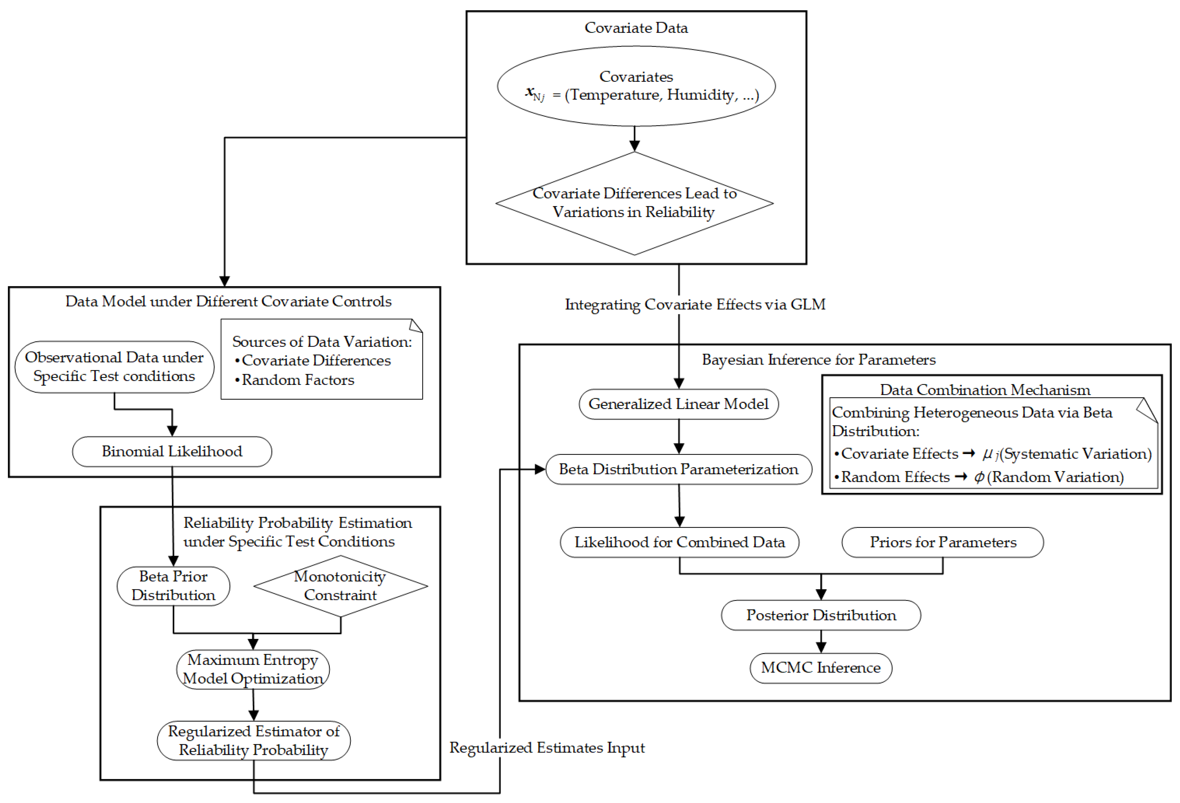
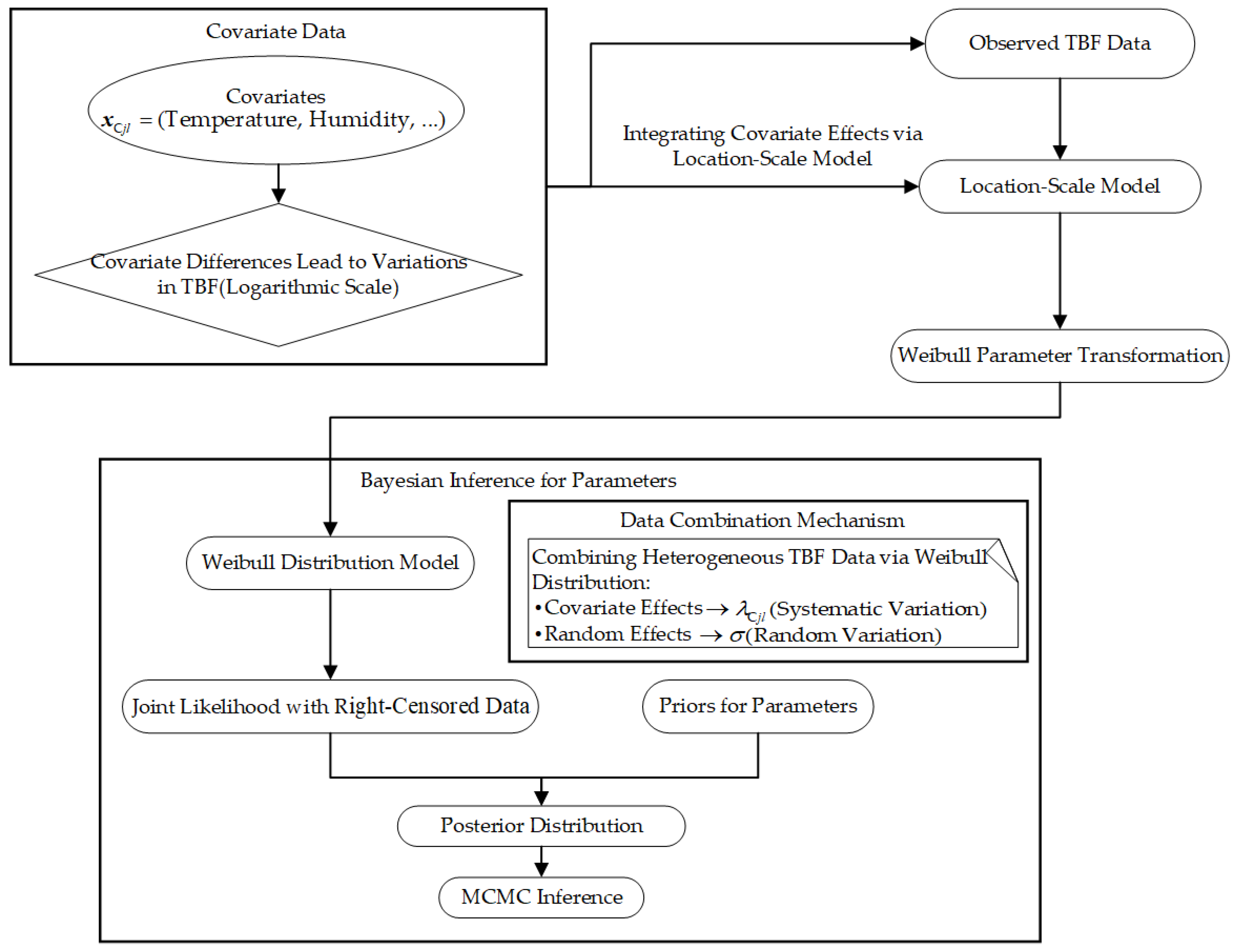
• Traditional Bayesian frameworks enable multi-source data combination through prior distribution; they rarely consider quantifying the intrinsic sources of heterogeneity. This work extends the Bayesian framework by embedding covariates via generalized linear model (GLM) and the location-scale regression model, quantitatively characterizing environmental impacts.
• Posterior inference employed the no-U-turn sampler (NUTS), an adaptive Hamiltonian Monte Carlo (HMC) variant within the MCMC framework. It automates tuning of leapfrog steps via recursive tree doubling, eliminating inefficient random-walk behavior inherent in traditional MCMC. This achieves faster convergence to target distribution.

The key innovations of this research are summarized below:

(1)

A multi-type data-driven phased assessment modeling method. By partitioning mission phases according to subsystem type characteristics, this approach establishes a granular mapping between data types and evaluation models, laying a foundation for high-resolution mission reliability analysis.

(2)

A dynamic optimization model with physical constraints for time-varying reliability parameters. Integrating the maximum entropy criterion with the monotonic reliability degradation principle during hyperparameter estimation, this innovation effectively mitigates parameter distortion under non-stationary data conditions.

(3)

A covariate-embedded data fusion evaluation methodology. By embedding covariates into Bayesian models for historical data combination, this innovation effectively addresses the practical engineering challenges of heterogeneous test data fusion while quantifying environmental influences.

The remainder of this paper is organized as follows: Section 2 presents the construction method for the phased RBD of the VMLS and details the proposed mission reliability assessment model. Section 3 employs a simulation case and a real-world engineering case to validate the proposed methodology. The final section presents four key conclusions and outlines future research directions.

2. Materials and Methods

2.1. Construction of Phased RBD

The dynamic assessment requirements for mission reliability in equipment operational testing necessitate phased modeling methodology. Equipment completes missions through multi-phase task execution. In each phase, different subsystems are activated to fulfill stage-specific objectives, which may generate heterogeneous data types. Different data types demand specialized reliability models. This section takes VMLS as an example and constructs the phased RBD shown in Figure 1, according to the definition of mission profiles [21] and considering the characteristics of VMLS operational testing. The mission profile is assumed to be divided into four functional phases: maneuver deployment (Phase 00), position deployment (Phase 01), missile ignition (Phases 11, 21, and 31), and missile flight (Phases 12, 22, and 32). Each phase accomplishes operational objectives through corresponding mission subsystems: the chassis (C) and navigation module (N) support battlefield mobility, the hydraulic system (H) completes launcher leveling, the ignition circuit (F) triggers sequential launches of three missiles (M1–M3), and the missiles perform designated functions during flight phases (e.g., approaching targets within allowable trajectory envelopes).

The diagram also annotates data types within the operational testing framework. “Time” in time-between-failures (TBFs) data is defined as generalized operational time, utilizing the most mission-relevant metric (e.g., hours, mileage for mobility phases). This ensures reliability metrics are meaningful and directly tied to mission execution stress, rather than solely calendar time. “Failure” is strictly defined as an operational mission failure (OMF), which is a critical failure directly preventing the accomplishment of the current phase’s essential objective and leading to mission termination. This OMF definition focuses on failures impacting mission essential functions (MEFs) at the mission-critical level. While other failure classifications exist, including essential function failures (EFFs) that affect specific MEFs without necessarily terminating the mission and non-essential function failures (NEFFs) impacting performance without loss of MEFs, the framework consistently applies the OMF standard for assessing mission reliability across all phases.

According to the IEC 60300-3-11:2009 standard [22] published by the International Electrotechnical Commission, mission subsystems can be classified into three categories based on operational modes:

• Continuous operation systems: Include subsystems C, N, and H. These subsystems operate persistently throughout a phase, accumulating operational exposure metrics and generating time-dependent failure data. Aircraft engines (during flight), conveyor belts, data center servers, and analogous systems also fall within this category. Critical faults in C and H can be immediately detected, while subsystem N requires scheduled inspections. Consequently, the data generated by subsystem N differs from that of C and H: the former produces success/failure data with varying success rates, whereas the latter generates TBF data.
• Demand-operated systems: Include subsystem F. Maintaining quiescent operation (standby/dormant mode) during extended periods with transition to active state only upon defined triggering events, such systems exhibit characteristically transient functional execution phases and consequently undergo reliability assessment via binary success/failure data without operational time monitoring or feasible recording. Fire alarm units, automotive starter motors, and pilot ejection systems are likewise classified within this paradigm.
• Pulse-operated systems: Include subsystems M1–M3. Such systems undergo exceptionally high peak loads or stresses within vanishingly brief durations (millisecond to second scale), subsequently persisting in low-load or standby states for extended periods. This operational paradigm is characterized by extreme instantaneous power/stress density juxtaposed with markedly diminished average power/stress levels. Electromagnetic railguns, pyrotechnic airbag inflators, and surge protective devices are also classified within this domain. Missiles further fall into the category of non-repairable systems that produce binary outcome data structurally equivalent to that of subsystem F.

Under operational testing conditions, the construction of the phased RBD should adhere to the principles of functional aggregation and hierarchical compression, differentiating phases and subsystems with distinctly different characteristics to lay the groundwork for targeted modeling. Furthermore, the established block diagram facilitates multi-path mission flow analysis (e.g., three missile launch branches) and dynamic termination mechanism simulation (termination upon mission completion) within the operational testing framework, thereby aligning with the operational censoring characteristics inherent to real-world combat scenarios.

2.2. Model Description

Mission reliability assessment in operational testing should transcend the limitations of traditional single data-type approaches and static mission path assumptions by constructing an assessment framework that integrates differentiated modeling of mission subsystems and multi-path mission synthesis. To this end, this section first develops reliability assessment models tailored to the distinct data characteristics of each mission subsystem, followed by the integration of assessment results at the mission profile level.

2.2.1. Reliability Assessment Model for Mission Subsystems

During the maneuver deployment phase (Phase 00), the navigation module (N) and chassis (C) form a series system. The reliability data generation process of subsystem N, which features delayed failure inspection mechanisms, significantly differs from that of the real-time responsive chassis system. Assuming N homogeneous VMLS units participate in the test with failure inspection conducted at identical frequencies, the following key parameters are defined:

$s_{\mathrm{N}k}$: Time duration from the previous failure restoration (including time zero) to the k-th inspection ($k=1,\dots ,n_{\mathrm{N}}$) within the interval between two detected failures, including the period before the first failure inspection.

$M_{\mathrm{N}k}$: Number of failure inspections recorded at $s_{\mathrm{N}k}$.

$b_{\mathrm{N}k}$: Number of inspections at which subsystem N remained in a normal state when inspections were conducted.

Assuming perfect failure detection, negligible repair time, and as-new restoration, a binomial probability model for $b_{\mathrm{N}k}$ can be established as

$$\mathrm{P}\left\{X_{\mathrm{N}}=b_{\mathrm{N}k}\right\}=\left(\begin{array}{c}{M}_{\mathrm{N}k}\\ b_{\mathrm{N}k}\end{array}\right)R_{\mathrm{N}k}^{b_{\mathrm{N}k}}{\left(1-R_{\mathrm{N}k}\right)}^{M_{\mathrm{N}k}-b_{\mathrm{N}k}}$$

(1)

Figure 2 illustrates the schematic diagram of the data generation process for four navigation modules. The diagram includes the following features:

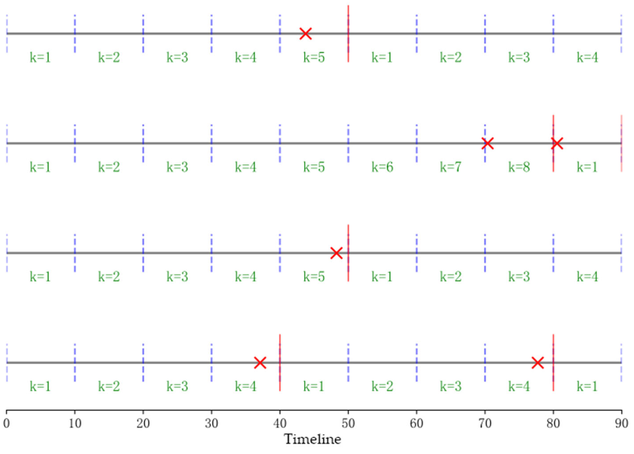
• Four horizontal solid lines representing timelines;
• Vertical dashed lines indicating failure inspection points;
• “×” symbols marking fault occurrences;
• Vertical red solid lines denoting failure restoration points.

In this case, the maximum value of $n_N$ is 8.

In theory, the reliability parameter $R_{Nk}$ in the binomial distribution should exhibit a strictly monotonic decreasing trend as k increases. However, employing traditional maximum likelihood estimation (MLE) to determine $R_{Nk}$ may lead to two critical issues:

(1)

Physical violation. Due to the stochastic nature of failure occurrences, estimated $R_{Nk}$ values might contradict physical feasibility. For instance, as shown in Figure 2, the reliability estimates for k = 5 and k = 6 yield implausible values of 0.33 and 1, respectively.

(2)

Non-continuity. The reliability function of the series system is not a time-dependent continuous function.

To address the first issue, a constrained optimization framework integrating Bayesian theory and information entropy principles [23] can be applied. This approach enforces the monotonic decreasing principle on both prior and posterior distributions of $R_{Nk}$. The Beta distribution is selected as the prior distribution for it, owing to its mathematical suitability for characterizing uncertainty in probability parameters. Its probability density function (PDF) is defined as:

$$\pi \left(R_{\mathrm{N}k}\left|a_{\mathrm{N}k},d_{\mathrm{N}k}\right.\right)={\displaystyle \frac{1}{\mathrm{B}\left(a_{\mathrm{N}k},d_{\mathrm{N}k}\right)}}{R}_{\mathrm{N}k}^{a_{\mathrm{N}k}-1}{\left(1-R_{\mathrm{N}k}\right)}^{d_{\mathrm{N}k}-1}$$

(2)

where $\mathrm{B}\left(\cdot \right)$ denotes the Beta function, with $a_{Nk}>0$ and $d_{Nk}>0$. The mathematical expectation of this distribution is expressed as:

$$\mathrm{E}(R_{\mathrm{N}k})={\displaystyle \frac{a_{\mathrm{N}k}}{a_{\mathrm{N}k}+d_{\mathrm{N}k}}}$$

(3)

By applying Bayes’ theorem in conjunction with Equation (2) and the test data $\left(M_{\mathrm{N}k},b_{\mathrm{N}k}\right)$, the posterior distribution of $R_{\mathrm{N}k}$ can be derived. The mathematical expectation of this distribution corresponds to the posterior estimate of $R_{\mathrm{N}k}$ under squared loss, expressed as:

$${\widehat{R}}_{\mathrm{N}k}={\displaystyle \frac{a_{\mathrm{N}k}+b_{\mathrm{N}k}}{a_{\mathrm{N}k}+d_{\mathrm{N}k}+M_{\mathrm{N}k}}}$$

(4)

To ensure the physical plausibility of reliability estimates, both the expected value $\mathrm{E}(R_{\mathrm{N}k})$ and the estimator ${\widehat{R}}_{\mathrm{N}k}$ are required to exhibit a monotonically decreasing trend as k increases. Consequently, a maximum entropy constrained optimization model is constructed as follows:

$$\begin{array}{l}\hspace{1em}\hspace{1em}\hspace{1em}\hspace{1em}\hspace{1em}\hspace{1em}\hspace{1em}\hspace{1em}\hspace{1em}\max H_{\mathrm{N}(k+1)}\\ \mathrm{s}.\mathrm{t}.\left\{\begin{array}{l}{\displaystyle \frac{a_{\mathrm{N}k}}{a_{\mathrm{N}k}+d_{\mathrm{N}k}}}-{\displaystyle \frac{a_{\mathrm{N}(k+1)}}{a_{\mathrm{N}(k+1)}+d_{\mathrm{N}(k+1)}}}>0 \\ {\displaystyle \frac{a_{\mathrm{N}k}+b_{\mathrm{N}k}}{a_{\mathrm{N}k}+d_{\mathrm{N}k}+M_{\mathrm{N}k}}}-{\displaystyle \frac{a_{\mathrm{N}(k+1)}+b_{\mathrm{N}(k+1)}}{a_{\mathrm{N}(k+1)}+d_{\mathrm{N}(k+1)}+M_{\mathrm{N}(k+1)}}}>0\\ a_{\mathrm{N}(k+1)}>0\\ d_{\mathrm{N}(k+1)}>0\end{array}\right.\end{array}$$

(5)

where $H_{\mathrm{N}k}$ denotes the information entropy of $\pi \left(R_{\mathrm{N}k}\left|a_{\mathrm{N}k},d_{\mathrm{N}k}\right.\right)$, which characterizes the uncertainty inherent to the prior distribution. Its mathematical expression is defined as:

$$\begin{array}{ll}{H}_{\mathrm{N}k}& =-{\displaystyle {\int }_0^1\pi \left(R_{\mathrm{N}k}\left|a_{\mathrm{N}k},d_{\mathrm{N}k}\right.\right)}\cdot \ln \pi \left(R_{\mathrm{N}k}\left|a_{\mathrm{N}k},d_{\mathrm{N}k}\right.\right)d{R}_{\mathrm{N}k}\\ & =\log B\left(a_{\mathrm{N}k},d_{\mathrm{N}k}\right)-(a_{\mathrm{N}k}-1)\phi (a_{\mathrm{N}k})-(d_{\mathrm{N}k}-1)\phi (d_{\mathrm{N}k})+\phi (a_{\mathrm{N}k}+d_{\mathrm{N}k})\left(a_{\mathrm{N}k}+d_{\mathrm{N}k}-2\right)\end{array}$$

(6)

Here, the digamma function $\phi (\cdot )$ is defined as ${\displaystyle \frac{\mathrm{d}}{\mathrm{d}x}}\log \mathsf{\Gamma }(\cdot )$, where Γ(⋅) denotes the Gamma function. The core principle of Equation (5) is to select the distribution with maximum information entropy under given constraints, thereby preserving the greatest uncertainty and enabling the most objective inferences consistent with empirical observations. For k = 1, the prior distribution of $R_{\mathrm{N}k}$ can be assigned a non-informative uniform distribution by setting hyperparameters $a_{\mathrm{N}1}=d_{\mathrm{N}1}=1$. Subsequent $a_{\mathrm{N}k}$ and $d_{\mathrm{N}k}$ are then sequentially solved using Equation (5), ultimately yielding the estimator ${\widehat{R}}_{\mathrm{N}k}$ in Equation (4).

Regarding the second issue mentioned earlier, since the reliability function can alternatively be modeled using a logistic regression framework with the TBF t of subsystem N as the covariate, the relationship between $R_{\mathrm{N}}$ and t is formulated as follows [24]:

$$\mathrm{logit}(R_{\mathrm{N}})=\ln \left({\displaystyle \frac{R_{\mathrm{N}}}{1-R_{\mathrm{N}}}}\right)={\theta }_{\mathrm{N}}+{\eta }_{\mathrm{N}}t$$

(7)

In operational testing, the analysis often requires supplementation of historical data, where discrepancies between supplemental and current datasets are governed by covariates such as temperature, humidity, and electromagnetic intensity. Therefore, the model in Equation (7) can be extended to a GLM as follows:

$$\mathrm{logit}(R_{\mathrm{N}j})={\theta }_{\mathrm{N}}+{\eta }_{\mathrm{N}}t+{\mathit{x}}_{\mathrm{N}j}^{\mathrm{T}}{\mathit{\beta }}_{\mathrm{N}}$$

(8)

Here, $R_{\mathrm{N}j}$ denotes the reliability probability of subsystem N in the j-th test, ${\theta }_{\mathrm{N}}$ is the fixed intercept, ${\eta }_{\mathrm{N}}$ is the time effect coefficient, ${\mathit{x}}_{\mathrm{N}j}$ represents the covariate vector for the j-th test, and ${\mathit{\beta }}_{\mathrm{N}}$ is the covariate effect coefficient vector. When data are collected from multiple tests, a data model $(t_{jk},{\widehat{R}}_{jk})$ can be established, where $t_{jk}$ indicates the time at the k-th inspection during the j-th test, and ${\widehat{R}}_{jk}$ is the estimated reliability probability at $t_{jk}$.

For the linear model specified in Equation (8), Bayesian methods can be employed to directly model the probability distribution of $R_{\mathrm{N}j}$, enabling flexible parameter estimation and uncertainty quantification. To achieve this, the prior distribution of $R_{\mathrm{N}j}$ is again defined as a conjugate Beta distribution [25], reparameterized as follows:

$$R_{\mathrm{N}j}~\mathrm{Beta}\left({\mu }_j\varphi ,(1-{\mu }_j)\varphi \right)$$

(9)

where ${\mu }_j$ is the expected value of the Beta distribution, and ϕ > 0 controls the dispersion of the distribution. Based on Equation (9), ${\mu }_j$ can be defined as:

$${\mu }_j={\mathrm{logit}}^{-1}\left({\theta }_{\mathrm{N}}+{\eta }_{\mathrm{N}}t+{\mathit{x}}_{\mathrm{N}j}^{\mathrm{T}}{\mathit{\beta }}_{\mathrm{N}}\right)$$

(10)

Based on the data pairs $(t_{jk},{\widehat{R}}_{jk})$, the joint likelihood function is formulated as:

$$L_{\mathrm{N}}={\displaystyle \prod _{j,k}\mathrm{Beta}\left({\widehat{R}}_{jk}\left|{\mu }_{jk}\varphi ,(1-{\mu }_{jk})\varphi \right.\right)}$$

(11)

where ${\mu }_{jk}$ is derived by substituting $t_{jk}$ into Equation (10). Furthermore, the joint posterior distribution can be formulated via Bayes’ theorem as follows:

$$\pi ({\theta }_{\mathrm{N}},{\eta }_{\mathrm{N}},{\mathit{\beta }}_{\mathrm{N}},\varphi \left|\mathrm{data}\right.)\propto L_{\mathrm{N}}\cdot \pi ({\theta }_{\mathrm{N}})\pi ({\eta }_{\mathrm{N}})\pi ({\mathit{\beta }}_{\mathrm{N}})\pi (\varphi )$$

(12)

Here, the four π(⋅) terms on the right-hand side of the proportionality symbol “∝” denote the prior distributions of the respective parameters. Since this posterior distribution does not admit a closed-form expression, the MCMC algorithm [26] can be employed to draw simulated samples of the parameters from the posterior distribution. These samples are then substituted into Equation (8) to generate samples of $R_{\mathrm{N}j}$, thereby enabling statistical inference on the reliability probability at each time point.

Although not explicitly declared, the derivation process in Equations (1)–(12) inherently embodies the concept of Bayesian hierarchical modeling. The essence of hierarchical modeling rests on a fundamental probability principle that the joint distribution of any random variable set can be decomposed into a chain of conditional probability structures. For random variables X, Y, and Z, their joint distribution satisfies $P(X,Y,Z)=P\left(Z\left|Y,X\right.\right)\cdot P\left(Y\left|X\right.\right)\cdot P\left(X\right)$, where P denotes the probability distribution. For the complex model in this study, the hierarchical modeling framework can be deconstructed into three stages [27]:

Stage 1. Data Model: $P(data\left|process,parameters\right.)={\displaystyle {\prod }_{j,k}\mathrm{Binomial}(b_{jk}\left|M_{jk},R_{jk}\right.)}$, where b_jk and M_jk denote the b_NK and M_Nk in the j-th test, respectively.

Stage 2. Process Model: $P(process\left|parameters\right.)={\displaystyle {\prod }_{j,k}\mathrm{Beta}(R_{jk}\left|{\mu }_j\varphi ,(1-{\mu }_j)\varphi \right.)}$

Stage 3. Parameter Model: $P(parameters)=\pi ({\theta }_{\mathrm{N}})\pi ({\eta }_{\mathrm{N}})\pi ({\mathit{\beta }}_{\mathrm{N}})\pi (\varphi )$

The objective of the standard Bayesian hierarchical model is to derive the posterior distribution via Bayes’ theorem:

$$\begin{array}{ll}P(process,parameters\left|data\right.)& \propto P(data\left|process,parameters\right.)\cdot P(process\left|parameters\right.)\\ & \cdot P(parameters)\end{array}$$

Within this framework, the reliability parameters ${\{R}_{jk}\}$ act as latent process variables. Direct MCMC sampling would require simultaneous estimation of high-dimensional ${\{R}_{jk}\}$ and parameter vector (${\theta }_{\mathrm{N}},{\eta }_{\mathrm{N}},{\mathit{\beta }}_{\mathrm{N}},\varphi$). This incurs a curse of dimensionality, manifesting as drastically reduced MCMC convergence speed and unstable parameter estimates. While preserving the statistical inference objective, estimating parameter vector (${\theta }_{\mathrm{N}},{\eta }_{\mathrm{N}},{\mathit{\beta }}_{\mathrm{N}},\varphi$), the proposed method restructures the computational path to overcome the dual challenges. Specifically, it merges the data model and process model from the conventional hierarchical framework into a regularized likelihood ${\prod }_{j,k }\mathrm{Beta}\left({\widehat{R}}_{jk}\left|{\mu }_{jk}\varphi ,(1-{\mu }_{jk})\varphi \right.\right)$, which reduces the sampling space from dim(${\{R}_{jk}\}$) + dim(${\theta }_{\mathrm{N}},{\eta }_{\mathrm{N}},{\mathit{\beta }}_{\mathrm{N}},\varphi$) to dim(${\theta }_{\mathrm{N}},{\eta }_{\mathrm{N}},{\mathit{\beta }}_{\mathrm{N}},\varphi$), where dim(•) denotes the dimensionality of the parameter space.

To more clearly visualize the modeling logic described above, Figure 3 systematically illustrates the entire process of covariate-embedded reliability modeling. Starting from covariate differences, it progresses through statistical model transformation and Bayesian inference to form a complete statistical inference chain.

For continuous operation systems (C/H), the TBF can be assumed to follow a two-parameter Weibull distribution, which is widely adopted in reliability engineering due to its flexibility and intrinsic connections with other distributions (e.g., exponential and Rayleigh distributions) [28]. Taking subsystem C as an example, its PDF and reliability function are respectively expressed as:

$$f_{\mathrm{C}}(t)={\displaystyle \frac{{\delta }_{\mathrm{C}}}{{\lambda }_{\mathrm{C}}}}{\left({\displaystyle \frac{t}{{\lambda }_{\mathrm{C}}}}\right)}^{{\delta }_{\mathrm{C}}-1}\exp \left[-{\left({\displaystyle \frac{t}{{\lambda }_{\mathrm{C}}}}\right)}^{{\delta }_{\mathrm{C}}}\right]$$

(13)

$$R_{\mathrm{C}}(t)=\exp \left[-{\left({\displaystyle \frac{t}{{\lambda }_{\mathrm{C}}}}\right)}^{{\delta }_{\mathrm{C}}}\right]$$

(14)

where λ_C denotes the scale parameter (characteristic life) and δ_C represents the shape parameter (failure mechanism characteristic). When multi-source test data are available, an environmental factor $\epsilon$_j can be introduced to model the TBF across tests as following a Weibull distribution with scale parameter ε_jλ_C and shape parameter δ_C. This implies that subsystem C maintains consistent failure mechanisms across different tests, while its characteristic life exhibits proportional relationships governed by $\epsilon$_j [19].

Analytical insights reveal that variations in characteristic life across tests primarily stem from factors such as temperature, humidity, and inherent quality variations in the systems. Consequently, through appropriate extensions of the location-scale model [29], the following relationship is derived:

$$\log (T_{\mathrm{C}jl})={\theta }_{\mathrm{C}}+{\mathit{x}}_{\mathrm{C}jl}^{\mathrm{T}}{\mathit{\beta }}_{\mathrm{C}}+\sigma {\upsilon }_{jl}$$

(15)

In Equation (15), $T_{\mathrm{C}jl}$ denotes the l-th TBF in the j-th test, ${\mathit{x}}_{\mathrm{C}jl}$ is the covariate vector, ${\theta }_{\mathrm{C}}$ represents the log-scale parameter of the baseline TBF, ${\mathit{\beta }}_{\mathrm{C}}$ is the covariate effect coefficient vector, ${\upsilon }_{jl}$ is the random error term, and $\sigma$ is the scale parameter adjusting the variability of the error term. If the PDF of ${\upsilon }_{jl}$ is defined as g(x), the PDF of $\log (T_{\mathrm{C}jl})$ can be derived through transformation as:

$$f_1\left(\log t_{\mathrm{C}jl}\right)={\displaystyle \frac{1}{\sigma }}g\left({\displaystyle \frac{\log t_{\mathrm{C}jl}-{\theta }_{\mathrm{C}}-{\mathit{x}}_{\mathrm{C}j}^{\mathrm{T}}{\mathit{\beta }}_{\mathrm{C}}}{\sigma }}\right)$$

(16)

Furthermore, when ${\upsilon }_{jl}$ follows a standard extreme value distribution, the covariate-dependent form of the Weibull distribution for $T_{\mathrm{C}jl}$ can be derived through variable substitution as follows:

$$f_2(t_{\mathrm{C}jl})={\displaystyle \frac{1}{\sigma t_{\mathrm{C}jl}}}\exp \left({\displaystyle \frac{\log t_{\mathrm{C}jl}-{\theta }_{\mathrm{C}}-{\mathit{x}}_{\mathrm{C}jl}^{\mathrm{T}}{\mathit{\beta }}_{\mathrm{C}}}{\sigma }}\right)\exp \left[-\exp \left({\displaystyle \frac{\log t_{\mathrm{C}jl}-{\theta }_{\mathrm{C}}-{\mathit{x}}_{\mathrm{C}j}^{\mathrm{T}}{\mathit{\beta }}_{\mathrm{C}}}{\sigma }}\right)\right]$$

(17)

Under these conditions, the parameters of the Weibull distribution can be analytically derived as:

$${\delta }_{\mathrm{C}}={\displaystyle \frac{1}{\sigma }},{\lambda }_{\mathrm{C}jl}=\exp \left({\theta }_{\mathrm{C}}+{\mathit{x}}_{\mathrm{C}jl}^{\mathrm{T}}{\mathit{\beta }}_{\mathrm{C}}\right)$$

(18)

Accounting for censored data, a joint likelihood function across multiple (J) tests can be constructed as:

$$L_{\mathrm{C}}={\displaystyle \prod _{j=1}^J{\displaystyle \prod _{l\in {\mathrm{D}}_j}\frac{1}{\sigma {\lambda }_{\mathrm{C}jl}}{\left(\frac{t_{\mathrm{C}jl}}{{\lambda }_{\mathrm{C}jl}}\right)}^{\frac{1}{\sigma }-1}\exp \left[-{\left(\frac{t_{\mathrm{C}jl}}{{\lambda }_{\mathrm{C}jl}}\right)}^{\frac{1}{\sigma }}\right]}\cdot {\displaystyle \prod _{l\in {\mathrm{C}}_j}\exp \left[-{\left(\frac{t_{\mathrm{C}jl}}{{\lambda }_{\mathrm{C}jl}}\right)}^{\frac{1}{\sigma }}\right]}}$$

(19)

where $D_j$ and $C_j$ denote the failure dataset and right-censored dataset, respectively, in the j-th test. Using Bayes’ theorem, the joint posterior distribution can be derived as follows:

$$\pi \left({\theta }_{\mathrm{C}},{\mathit{\beta }}_{\mathrm{C}},\sigma ,\left|\mathrm{data}\right.\right)\propto \pi ({\theta }_{\mathrm{C}})\pi ({\mathit{\beta }}_{\mathrm{C}})\pi (\sigma )L_{\mathrm{C}}$$

(20)

Similar to the approach applied to Equation (12), the MCMC algorithm can be utilized to infer parameters and reliability probability.

To visually encapsulate the aforementioned modeling logic, Figure 4 illustrates the entire process of covariate-embedded reliability analysis. It sequentially integrates TBF variations influenced by covariates (with random effects additionally contributing to variability), location-scale model-based parameter mapping, and Bayesian inference with data combination.

For demand-operated systems (F) and pulse-operated systems (M1–M3), their test data exhibit the following distinctive characteristics compared to other systems discussed in this study:

(1)

Both historical and current test data are sparse due to either the inherent high reliability of these subsystems or cost constraints in testing, resulting in extremely scarce failure incidents.

(2)

Failures are predominantly triggered by transient events such as electromagnetic pulse interference or mechanical shocks, rather than cumulative effects of covariates.

(3)

Only binary outcomes (success/failure) are recorded, which prevents the acquisition of precise stress profile data over time.

Under these conditions, continued application of covariate-dependent regression models would lead to unstable parameter estimates or even overfitting due to data sparsity. For such systems, expert knowledge serves as a critical form of unstructured prior information [30]. Within the Bayesian framework, this expertise can be integrated into prior distributions, enabling joint posterior inference of relevant parameters by synthesizing operational testing outcomes. Taking subsystem F as an example, the prior distribution for the success probability (i.e., reliability probability) in Bernoulli trials can be specified as a Beta distribution:

$$\pi \left(R_{\mathrm{F}}\left|a_{\mathrm{F}},b_{\mathrm{F}}\right.\right)={\displaystyle \frac{1}{B\left(a_{\mathrm{F}},b_{\mathrm{F}}\right)}}{R}_{\mathrm{F}}^{a_{\mathrm{F}}-1}{\left(1-R_{\mathrm{F}}\right)}^{b_{\mathrm{F}}-1}$$

(21)

The hyperparameters in the equation should satisfy high-reliability constraints, specifically:

$$a_{\mathrm{F}}>1,0<b_{\mathrm{F}}\le 1$$

(22)

As shown in Figure 5, this constraint ensures that the PDF of the Beta distribution is a monotonically increasing function, reflecting the engineering consensus that the reliability probability $R_{\mathrm{F}}$ is highly likely to approach 1.

For the test data $D_{\mathrm{F}}=\left(n_{\mathrm{F}},s_{\mathrm{F}}\right)$, where $n_{\mathrm{F}}$ and $s_{\mathrm{F}}$ represent the count of Bernoulli trials and successful operations, respectively, the likelihood function is given by:

$$L\left(R_{\mathrm{F}}\right)=\left(\begin{array}{c}{n}_{\mathrm{F}}\\ s_{\mathrm{F}}\end{array}\right)R_{\mathrm{F}}^{s_{\mathrm{F}}}{\left(1-R_{\mathrm{F}}\right)}^{n_{\mathrm{F}}-s_{\mathrm{F}}}$$

(23)

By applying Bayes’ theorem to combine Equations (21) and (23), the posterior distribution can be derived as:

$$\pi \left(R_{\mathrm{F}}\left|D_{\mathrm{F}}\right.\right)={\displaystyle \frac{R_{\mathrm{F}}^{a_{\mathrm{F}}+s_{\mathrm{F}}-1}{\left(1-R_{\mathrm{F}}\right)}^{b_{\mathrm{F}}+n_{\mathrm{F}}-s_{\mathrm{F}}-1}}{B\left(a_{\mathrm{F}}+s_{\mathrm{F}},b_{\mathrm{F}}+n_{\mathrm{F}}-s_{\mathrm{F}}\right)}}$$

(24)

Assuming the expert knowledge is the estimated reliability probability ${\widehat{R}}_{\mathrm{F}}$ of subsystem F, a maximum entropy constrained model can be established to integrate this information into the Beta prior distribution while mitigating subjectivity risks:

$$\begin{array}{l}\max H(a_{\mathrm{F}},b_{\mathrm{F}})\\ \mathrm{s}.\mathrm{t}. \mathrm{E}\left(R_{\mathrm{F}}\right)={\widehat{R}}_{\mathrm{F}};\\ a_{\mathrm{F}}>1,0<b_{\mathrm{F}}\le 1.\end{array}$$

(25)

where $\mathrm{E}\left(R_{\mathrm{F}}\right)=a_{\mathrm{F}}/\left(a_{\mathrm{F}}+b_{\mathrm{F}}\right)$ is the expected value of the prior distribution of $R_{\mathrm{F}}$. The information entropy $H(a_{\mathrm{F}},b_{\mathrm{F}})$ can be calculated using the method outlined in Equation (6). Hyperparameters $a_{\mathrm{F}}$ and $b_{\mathrm{F}}$ are then determined via Equation (25), and inference for $R_{\mathrm{F}}$ is performed using the MCMC algorithm.

2.2.2. MCMC-Based Posterior Inference and Model Validation

As discussed earlier, the MCMC algorithm is employed to perform posterior inference for the parameters of interest based on their joint posterior distributions (e.g., θ_N, η_N, β_N, ϕ in Equation (12) and θ_C, β_C, σ in Equation (20)). Specifically, the NUTS is employed to generate posterior samples from these distributions. As an advanced extension of HMC [31], it leverages first-order gradient information to construct parameter space trajectories, effectively mitigating the random-walk behavior and hyperparameter sensitivity inherent in conventional MCMC methods. Its recursive tree-building mechanism dynamically terminates trajectories upon detecting U-turns in the Hamiltonian dynamics, while the dual-averaging algorithm autonomously optimizes the step size ϵ during sampling. Together, these adaptive features eliminate manual tuning dependencies and scale computational effort to match the geometry of high-dimensional posterior distributions, thus achieving accelerated convergence. Let $\Theta$ denote the parameter vector requiring posterior inference. The Bayesian estimate of $\Theta$ can then be straightforwardly derived from posterior samples. The sampling procedure of NUTS integrates Hamiltonian dynamics simulation with path termination strategy from HMC, which comprises the following steps:

Step 1: Parameter and momentum initialization. Initialize the vector $\Theta$ to ${\Theta }^{(0)}$ and draw momentum vector r from a standard multivariate normal distribution Normal(0, I), where the dimensionality of r matches that of $\Theta$.

Step 2: Hamiltonian system definition. Construct the Hamiltonian energy function:

$$H\left(\Theta ,r\right)=-\log \pi (\Theta \left|D_a\right.)+{\displaystyle \frac{1}{2}}{\displaystyle \sum _{k^{\prime }}{\mathit{r}}_{k^{\prime }}^2}$$

where $-\log \pi (\Theta \left|D_a\right.)=-\log \pi (D_a\left|\Theta \right.)-{\displaystyle {\sum }_{k^{\prime }}\log \pi ({\Theta }_{k^{\prime }})}$ represents the negative log-posterior, and k′ is the element index within the corresponding vector. The log-posterior gradient is computed as partial derivatives:

$${\nabla }_{\Theta }\log \pi (\Theta \left|D_a\right.)=\left(\left\{{\displaystyle \frac{\mathcal{\partial }\log \pi }{\mathcal{\partial }{\Theta }_{k^{\prime }}}}\right\}\right)$$

Step 3: Recursive trajectory construction. Starting from the current state ($\Theta$,r), execute leapfrog integration with step size $\epsilon$ through iterative updates:

• Half-step momentum update: ${\mathit{r}}_{k^{\prime }}\leftarrow {\mathit{r}}_{k^{\prime }}+{\displaystyle \frac{\epsilon }{2}}\cdot {\displaystyle \frac{\mathcal{\partial }\log \pi }{\mathcal{\partial }{\Theta }_{k^{\prime }}}}$;
• Full-step position update: ${\Theta }_{k^{\prime }}\leftarrow {\Theta }_{k^{\prime }}+\epsilon \cdot {\mathit{r}}_{k^{\prime }}$;
• Half-step momentum completion: ${\mathit{r}}_{k^{\prime }}\leftarrow {\mathit{r}}_{k^{\prime }}+{\displaystyle \frac{\epsilon }{2}}\cdot {\displaystyle \frac{\mathcal{\partial }\log \pi }{\mathcal{\partial }{\Theta }_{k^{\prime }}}}$.

Trajectory expansion employs a bidirectional recursive strategy. The termination condition activates when the dot product between position difference vectors and momentum satisfies:

$${\displaystyle {\sum }_{k^{\prime }}\left({\Theta }_{k^{\prime }}^{+}-{\Theta }_{k^{\prime }}^{-}\right)\cdot {\mathit{r}}_{k^{\prime }}^{-}}<0\mathrm{or}{\displaystyle {\sum }_{k^{\prime }}\left({\Theta }_{k^{\prime }}^{+}-{\Theta }_{k^{\prime }}^{-}\right)\cdot {\mathit{r}}_{k^{\prime }}^{+}<0}$$

where ${\Theta }_{k^{\prime }}^{\pm }$ denote endpoint states. The effective trajectory length L follows geometric progression L = $2^{j^{\prime }}-1$ for recursion depth j′.

Step 4: State selection. Draw $u~$$\mathrm{Uniform}\left[0,\exp \left(-H(\Theta ,\mathit{r})\right)\right]$ and select states satisfying $H({\Theta }^{\prime },r^{\prime })\le -\log u$. A new state ${\Theta }_{\mathrm{new}}$ is then sampled uniformly from valid candidates.

Step 5: Adaptive step-size tuning. Dynamically adjust $\epsilon$ via dual averaging:

$$\log {\epsilon }_{t+1}=\mu -{\displaystyle \frac{\sqrt{t}}{\gamma }}{\overline{\delta }}_t,\mu =\log (10{\epsilon }_0)\text{}$$

where ${\overline{\delta }}_t$ is the exponentially weighted average of acceptance probability deviation, $\gamma$ is the adaptive tuning rate, and $\mu$ is the long-term target for $\log \epsilon$, with ${\epsilon }_0$ denoting the initial step size.

After obtaining posterior samples of the parameter vector $\Theta$ through the sampling procedure, posterior inference can be conducted for individual elements within the vector (i.e., separate parameters), primarily consisting of point estimation and interval estimation. The ultimate objective is to derive posterior inferences for the reliability of each subsystem under operational testing conditions.

For subsystems N and C, given mission time and covariate values under operational testing conditions, the posterior samples of reliability probability are derived from the parameter posterior samples through the functional relationships (Equation (8) for subsystem N, and Equation (14) for subsystem C). For subsystem F, reliability probability itself constitutes the target parameter, thus requiring no transformation.

In summary, all statistical inferences for parameters and reliability probability are based on posterior samples obtained via sampling. Let ${\left\{{\rho }^{\left(v\right)}\right\}}_{v=1}^N$ denote the posterior sample set, where N is the sample size. The Bayesian point estimate is computed as the sample mean ${\displaystyle \frac{1}{N}}{\sum }_{v=1}^N{\rho }^{\left(v\right)}$.

For interval estimation, this study employs the highest posterior density (HPD) interval, which prioritizes inclusion of values with maximal posterior density while maintaining coverage probability, thereby achieving minimal interval length [32]. The computational procedure consists of two steps:

Step 1: Arrange samples $\left\{{\rho }^{\left(v\right)}\right\}$ in ascending order as ${\rho }_{\left(1\right)}\le {\rho }_{\left(1\right)}\le \cdots {\rho }_{\left(N\right)}$.

Step 2: Calculate coverage sample size $z=⌈N\cdot (1-\alpha )⌉$, where $⌈·⌉$ denotes the ceiling function. Compute lengths L_v = ${\rho }_{(v+z-1)}-{\rho }_{\left(v\right)}$ for all contiguous intervals $\left[{\rho }_{\left(v\right)},{ \rho }_{(v+z-1)}\right]$. The interval corresponding to minimal L_v is selected as the (1 − α) × 100% HPD interval.

Posterior predictive checks are essential for assessing model validity, with the Bayesian posterior predictive p-values (ppp) serving as a useful metric for evaluating the model–data fit. For each posterior draw of the model parameters, a set of posterior predictive data matching the size of the observed data is generated. A chosen statistic (e.g., mean and median) for both the observed data and posterior predictive data, denoted as $S_{obs}^{\left(v\right)}$ and $S_{rep}^{\left(v\right)}$, is computed. The ppp is calculated as the proportion of $S_{rep}^{\left(v\right)}$ exceeding $S_{obs}$ [33]:

$$p_{\mathrm{B}}={\displaystyle \frac{1}{N}}{\displaystyle \sum _{v=1}^N\mathrm{I}\left(S_{\mathrm{rep}}^{(v)}\ge S_{\mathrm{obs}}\right)}$$

where $\mathrm{I}\left(\cdot \right)$ is the indicator function (equal to 1 if the condition holds, otherwise 0). A $p_B$ value close to 0.5 indicates that the $S_{obs}$ lies near the center of the posterior predictive statistics, suggesting that the model provides an adequate fit.

2.2.3. Multi-Path Mission Reliability Assessment

Following the independent reliability modeling and statistical inference of subsystems across phases within the mission profile, the mission reliability assessment fundamentally involves probabilistic integration under multi-path dynamic execution scenarios. Under operational testing conditions, mission reliability depends both on the independent performance of phase-specific reliability and the weighting and contribution of different mission paths to the overall reliability. With the mission success criterion defined as “two missiles successfully striking the target” and the success criterion for the missile flight phase distinguished as “approaching the target within allowable trajectory envelopes”, the mission reliability assessment must account for the following operational paths:

Path 1: M1 misses the target but proceeds through all mission phases.

Path 2: M1 and M2 both strike the target, triggering early termination of subsequent launches.

Path 3: M1 strikes the target while M2 misses, requiring continuation of remaining mission phases.

Let $R_m$ denote the mission reliability probability of the VMLS in phase m. The mission reliability probability for each path is then calculated as follows:

$$\left\{\begin{array}{l}{R}_{s1}=R_{00}{R}_{01}{R}_{11}{R}_{21}{R}_{31}{R}_{12}{R}_{22}{R}_{32}\\ R_{s2}=R_{00}{R}_{01}{R}_{11}{R}_{21}{R}_{12}{R}_{22}\\ R_{s3}=R_{s1}\end{array}\right.$$

(26)

If the missile’s accuracy is quantified by the hit probability p, the system-level mission reliability probability is defined as:

$$R_s=\left(1-p\right)R_{s1}+p^2{R}_{s2}+p\left(1-p\right)R_{s3}$$

(27)

Based on the posterior reliability samples of each subsystem obtained through the methodology described in Section 2.2.1, the posterior distribution of $R_s$ can be simulated using Equation (27), thereby enabling statistical inference on it.

3. Results and Discussion

To systematically validate the effectiveness and engineering applicability of the proposed method, we establish a dual verification framework comprising a simulation scenario and a field deployment case.

3.1. Simulation Scenario Validation

This subsection conducts simulation validation using the binomial data processing method for subsystem N described in Section 2.2.1 as an example, temporarily excluding the covariate vector ${\mathit{x}}_{\mathrm{N}j}$. Based on the logistic regression model defined in Equation (7), the reliability function is formulated as:

$$R_{\mathrm{N}}(t)={\displaystyle \frac{1}{1+\exp \left[-\left({\theta }_{\mathrm{N}}+{\eta }_{\mathrm{N}}t\right)\right]}},{\theta }_{\mathrm{N}}>0,{\eta }_{\mathrm{N}}<0$$

(28)

It can be shown that the TBF follows a logistic distribution with location parameter $-{\theta }_{\mathrm{N}}/{\eta }_{\mathrm{N}}$ and scale parameter $-1/{\eta }_{\mathrm{N}}$. Parameter true-value combinations are set as $\left({\theta }_{\mathrm{N}},{\eta }_{\mathrm{N}}\right)\in$ {(2, −0.05), (1.8, −0.04), (3.5, −0.03), (4.3, −0.02)} to simulate equipment scenarios with distinct failure rate characteristics.

Assume four equipment units participate in the test. Taking $\left({\theta }_{\mathrm{N}},{\eta }_{\mathrm{N}}\right)$ = (2, −0.05) as an example, the total test duration is set to T = 90 generalized time units with inspection intervals Δt = 5. Simulated TBF following the logistic distribution are then generated along the timeline shown in Figure 2 to determine failure occurrence points. The compiled data are summarized in

Table 1. Simulation data summary table.

k	${\mathit{M}}_{\mathbf{N}\mathit{k}}$	${\mathit{b}}_{\mathbf{N}\mathit{k}}$	${\mathit{s}}_{\mathbf{N}\mathit{k}}$
1	12	10	5
2	9	8	10
4	8	8	20
5	8	7	25
6	6	5	30
7	4	3	35
12	3	3	60
13	2	0	65

.

In Table 1, data entries for k = 3 and k = 8, 9, 10, 11 are deemed invalid and excluded due to redundancy with k = 4 and k = 12, respectively. Following the methodology outlined in Section 2.2.1, the reliability probability for each valid k-value in Table 1 is estimated sequentially using Equations (4) and (5). Subsequently, posterior distribution sampling for ${\theta }_N$ and ${\eta }_{\mathrm{N}}$ is performed via Equation (12), yielding point estimates and 95% HPD intervals for both parameters.

For comparative analysis, the classical method [24] is applied to estimate these parameters. This method bypasses per-inspection reliability estimation and instead directly constructs a likelihood function based on the data pairs $\left(M_{\mathrm{N}k},b_{\mathrm{N}k}\right)$ by substituting Equation (28) into Equation (1). Posterior estimates of ${\theta }_{\mathrm{N}}$ and ${\eta }_{\mathrm{N}}$ are then derived using Bayes’ theorem and the NUTS.

During the execution of both methods, diffuse priors $\pi \left({\theta }_{\mathrm{N}}\right)$, $\pi \left({\eta }_{\mathrm{N}}\right)$ and $\pi \left(\varphi \right)$ are assigned a Normal(0,100), ensuring that the posterior distributions are primarily informed by the simulated data in Table 1. Multiple estimations are performed by varying T, $\Delta t$, and parameter combinations $\left({\theta }_{\mathrm{N}},{\eta }_{\mathrm{N}}\right)$. Comparative results are summarized in

Table 2. Simulation experiment results.

T	Δt	True Parameter Values	Parameter Estimation Results
			Proposed Method	Existing Method
90	5	${\theta }_{\mathrm{N}}=2$	1.983 [1.237, 2.763]	2.585 [1.266, 4.141]
		${\eta }_{\mathrm{N}}=-0.05$	−0.024 [−0.036, −0.013]	−0.018 [−0.048, 0.007]
300	20	${\theta }_{\mathrm{N}}=1.8$	1.852 [1.111, 2.595]	2.188 [0.930, 3.540]
		${\eta }_{\mathrm{N}}=-0.04$	−0.028 [−0.038, −0.017]	−0.033 [−0.059, −0.008]
400	20	${\theta }_{\mathrm{N}}=3.5$	3.468 [2.758, 4.270]	6.476 [3.712, 9.383]
		${\eta }_{\mathrm{N}}=-0.03$	−0.023 [−0.029, −0.017]	−0.043 [−0.065, −0.020]
500	25	${\theta }_{\mathrm{N}}=4.3$	3.144 [2.349, 4.037]	6.494 [2.900, 10.697]
		${\eta }_{\mathrm{N}}=-0.02$	−0.018 [−0.022, −0.003]	−0.023 [−0.041,−0.006]

.

From Table 2, three critical observations emerge. First, larger Δt values lead to increased estimation bias for both methods. However, the proposed method exhibits smaller bias, demonstrating stronger robustness against extended inspection intervals. This advantage arises from its constrained modeling approach that mitigates the temporal ambiguity in failure timing caused by larger intervals. Second, the proposed method achieves higher accuracy and precision when the absolute value of ${\eta }_{\mathrm{N}}$ is smaller. Mechanistically, smaller $\left|{\eta }_{\mathrm{N}}\right|$ corresponds to higher dispersion in TBF samples, leading to substantial fluctuations in reliability probability estimates at inspection points when relying solely on data. Existing methods perform poorly under such conditions. Third, the proposed method consistently yields narrower 95% HPD intervals, reflecting enhanced precision. From an engineering perspective, smaller $\left|{\eta }_{\mathrm{N}}\right|$ indicates slower degradation rates, validating the method’s applicability to reliability assessment scenarios for long-lifetime systems.

3.2. Field Deployment Case

This subsection conducts validation analysis based on desensitized test data from a specific VMLS. The operational testing was conducted through a live-force confrontation exercise at a high-altitude training ground, simulating an assault scenario where the red force attacked a heavily fortified defensive position of the blue force. The red force’s equipment under test included four identical VMLS, each armed with three surface-to-surface tactical missiles. Other equipment within the red force constituted several functional units, such as a target reconnaissance unit, a fire command and control unit, an integrated support unit, and so on. This equipment suite also encompassed additional offensive and accompanying defensive assets. Collectively, these elements, including the VMLS, constituted an integrated system-of-systems (SoS). The entire operational mission of the red force assault was divided into four phases: readiness level transition, maneuver and assembly, combat organization, and combat execution. Based on the SoS application plan, the operational testing tasks for the system-of-systems were delineated using the test profile shown in

Table 3. Test profile of the SoS.

Time Period	Evaluation Content	Operational Actions	Test Environment
			Terrain	Lighting	Meteorological
3 days	command and communication capability (CCC), integrated support capability (ISC), and in-service suitability (ISS)	readiness level transition	urban roads	daytime, nighttime	clear weather
12 days	CCC, maneuver and assault capability (MAC), and OS	maneuver and assembly	urban roads, moderately rolling roads	daytime, nighttime	clear weather, precipitation weather
2 days	reconnaissance and intelligence capability (RIC), CCC, OS, and SoS suitability	combat organization	moderately rolling roads	daytime, nighttime	precipitation weather
2 days	RIC, CCC, MAC, firepower strike capability (FSC), multi-domain defense capability, ISC, OS, SoS suitability, and ISS	combat execution	moderately rolling roads	daytime, nighttime	precipitation weather, fog weather

. This delineation integrated the mission profile, environmental profile, and the evaluation indicator system established for the operational testing.

3.2.1. Data Acquisition

The data collected and presented in this study encompass three core subsystems: chassis, navigation module, and missile. A summary of the dataset is provided in

Table 4. Dataset summary.

Mission Subsystem	Data Type	Data Distribution	Data Source	Sample Size (Censored)	Covariate Values
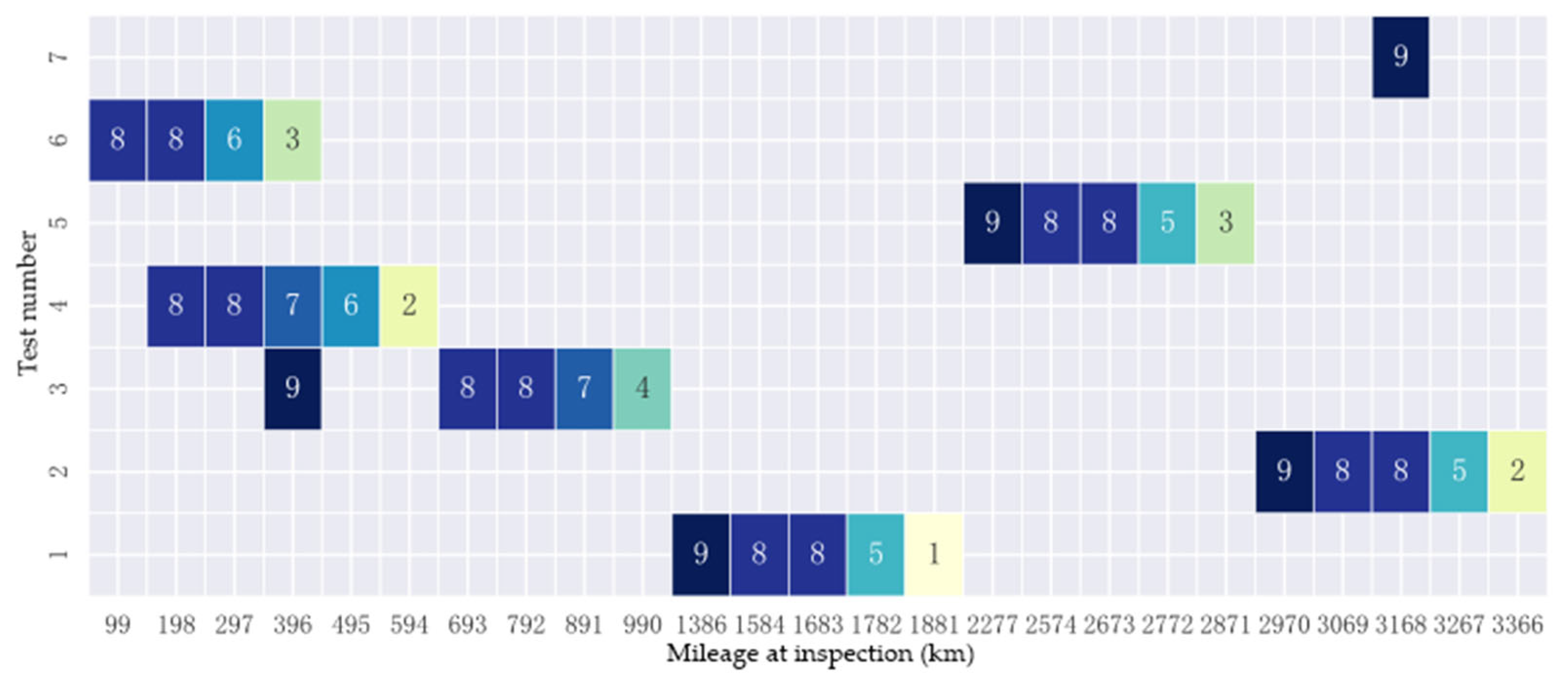
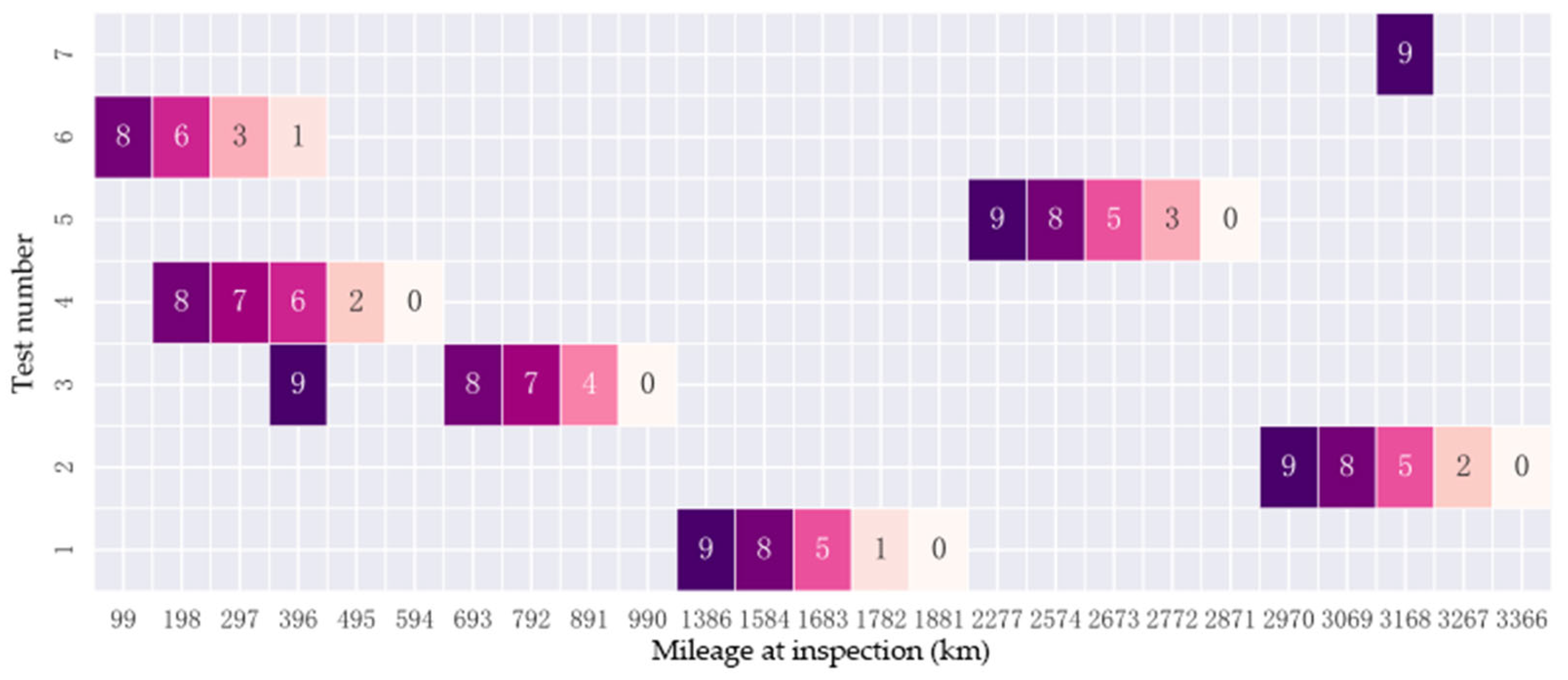
Navigation module	mileage from repair to failure inspection(km), number of success/total inspections	time-varying binomial distribution	operational testing	2 groups	relative humidity (RH): 0.62 temperature (Temp): −8.2 °C
			historical data	107 groups	RH: 0.20~0.75 Temp: −10 °C~35 °C
Chassis	TBF(km)	Weibull distribution	operational testing	6 (4) time records	RH: 0.62， Temp: −8.2 °C
			historical data	60 (18) time records	RH: 0.20~0.75 Temp: −10 °C~35 °C
Missile	success/failure	Bernoulli distribution	operational testing	6 trials	—
			expert knowledge	1 judgment	—

, where the covariate values for the operational testing represent averages calculated throughout the test period. The historical data are sourced from records obtained during multiple prior tests.

During operational testing, the navigation module yielded two sets of binomial data, each comprising four failure inspections. The recorded failure-free instances were four and two for the respective datasets. Historical data was incorporated, with Figure 6 and Figure 7 displaying heatmaps of the failure inspection counts and failure-free instances for the first 30 historical data of the navigation module.

Figure 8 illustrates the TBF data for the chassis, with distributions presented via boxplots. Test numbers 1~6 represent historical data, while number 7 corresponds to operational testing data. The operational testing yielded only six observations (including four right-censored data points), necessitating compensatory estimation by combining historical data.

Among the four tested VMLS units, two units each launched three missiles, resulting in five successful flight phase operations. Through organized expert discussions, the reliability probability of the missile flight phase was estimated to be 0.996.

3.2.2. Method Application

Based on the aforementioned data, the reliability of the navigation module, chassis, and missiles during their respective mission phases is assessed using the methodology described in Section 2.2.1.

For the navigation module, pre-estimated reliability probabilities at failure inspection points are derived using Equations (4) and (5), with the results shown in Figure 9. The historical data originate from 21 trials with varying covariate values, leading to significant variability in reliability probability estimates at identical time points.

A five-dimensional parameter vector $({\theta }_{\mathrm{N}},{\eta }_{\mathrm{N}},{\mathit{\beta }}_{\mathrm{N}},\varphi )$ is constructed, and diffuse priors are assigned as follows:

$$\begin{array}{l}{\theta }_{\mathrm{N}}~{\mathrm{HalfNormal}}^{+}(0,100)\\ {\eta }_{\mathrm{N}}~{\mathrm{HalfNormal}}^{-}(0,100)\\ {\mathit{\beta }}_{\mathrm{N}}~\mathrm{Normal}\left(\left(\begin{array}{c}0\\ 0\end{array}\right),\left(\begin{array}{cc}100& 0\\ 0& 100\end{array}\right)\right)\\ \varphi ~{\mathrm{HalfNormal}}^{+}(0,100)\end{array}$$

Subsequently, the parameters and reliability probabilities are estimated by combining Equations (8) and (12), leveraging Bayesian posterior sampling and the NUTS.

For the chassis, the test data shown in Figure 6 and covariate values from each test phase are first substituted into Equation (19). A four-dimensional parameter vector $({\theta }_{\mathrm{C}},{\mathit{\beta }}_{\mathrm{C}},\sigma )$ is defined, with diffuse priors assigned as follows:

$$\begin{array}{l}{\theta }_{\mathrm{C}}~\mathrm{Normal}(0,100)\\ {\mathit{\beta }}_{\mathrm{C}}~\mathrm{Normal}\left(\left(\begin{array}{c}0\\ 0\end{array}\right),\left(\begin{array}{cc}100& 0\\ 0& 100\end{array}\right)\right)\\ \sigma ~{\mathrm{HalfNormal}}^{+}(0,100)\end{array}$$

The parameters are estimated using Equation (20), followed by calculating the parameters of the Weibull distribution for the chassis’ TBF during the operational testing phase by incorporating covariate values. Finally, reliability probability is inferred according to Equation (14).

For the missile, the hyperparameters $a_{\mathrm{F}}$ = 248.230 and $b_{\mathrm{F}}$ = 0.997 are determined based on Equation (25). Subsequently, the reliability probability (success rate) of the flight phase for an individual missile is estimated using the NUTS.

During the inference of parameters and reliability probabilities for the aforementioned subsystems, the NUTS was configured with four independent Markov chains. Each chain generated 3000 posterior samples, preceded by 1200 burn-in iterations for tuning. The sample acceptance rate was maintained at 0.9 to ensure sampling efficiency. Posterior estimates of the relevant parameters are summarized in

Table 5. Posterior estimates of parameters.

Parameter	Posterior Mean	Standard Deviation	HPD Interval (95%)
θN	13.457	0.678	[12.171, 14.683]
ηN	−0.006	0.0001	[−0.007, −0.006]
βN	(−0.019, 7.465)	(0.029, 0.386)	([−0.079, 0], [6.744, 8.176])
φ	12.282	1.127	[10.270, 14.492]
θC	8.640	0.071	[8.502, 8.722]
βC	(−0.157, 0.217)	(0.090, 0.088)	([−0.325, 0.015], [0.088, 0.044])
σ	0.395	0.053	[0.298, 0.494]

.

Table 6. Statistical report on convergence.

Parameter	MCSE Mean	MCSE SD	ESS Bulk	ESS Tail	R-Hat
θN	0.014	0.009	2459	3409	1.0
ηN	0	0	2461	3422	1.0
βN[1]	0	0	6076	6117	1.0
βN[2]	0.008	0.005	2466	3544	1.0
φ	0.017	0.012	4559	5185	1.0
θC	0.001	0.001	7414	8099	1.0
βC[1]	0.001	0.001	6919	8562	1.0
βC[2]	0.001	0.001	7537	8182	1.0
σ	0.001	0.001	7350	7408	1.0

presents the convergence diagnostics for all parameters in Table 5, where all values were generated PyMC 5.18.2, a Python 3.13.3 probabilistic programming library.

The explanations for the column headers in Table 6 are as follows:

• MCSE mean: Monte Carlo standard error of mean estimate
• MCSE SD: Monte Carlo standard error of standard deviation estimate
• ESS bulk: Effective sample size for distribution bulk
• ESS tail: Effective sample size for distribution tails
• R-hat: Gelman–Rubin statistic.

Three critical observations validate robust sampling performance and trustworthy parameter estimation:

(1)

ESS bulk values span 2459~7537 (all substantially surpassing 2000), while ESS tail encompasses 3409~8562 (all well above 3000). These metrics indicate sufficient sampling and high sampling efficiency.

(2)

For all parameters, the ratios of MCSE mean and MCSE SD to the standard deviation (SD) in Table 4 are relatively small, with the maximum observed ratios being 0.021 (β_N[2]: 0.008/0.386) and 0.019 (σ: 0.001/0.053). This demonstrates highly reliable estimation of both posterior means and dispersions.

(3)

All parameters exhibit R-hat values of exactly 1, indicating complete convergence of sampling chains. No systematic divergence emerges among four Markov chains during the iteration process.

Assume the reliability probability distributions for the hydraulic system (H) and ignition circuit (F) are specified as

$$R_{\mathrm{H}}~\mathrm{Beta}\left(15,0.2\right), R_{\mathrm{F}}~\mathrm{Beta}\left(16,0.3\right)$$

This implies their reliability probabilities have mathematical expectations of 0.987 and 0.982, with standard deviations of 0.028 and 0.032, respectively. Random samples of R_H and R_F can then be generated through probability distribution transformation.

Given that the operational mission mileage for the navigation module and chassis is 800 km, their mission reliability probabilities can be determined. Based on the random samples of subsystem mission reliability probabilities and assuming p = 0.8, the mission reliability probability of the VMLS is derived using the methodology described in Section 2.2.3 The estimation results for the reliability probabilities of the three subsystems and the VMLS are shown in Figure 10. For the navigation module and chassis, the reliability function curves and mission reliability probability estimates are explicitly plotted, indicated by red dashed lines and circular markers. As illustrated in Figure 10, the mission reliability probability of the navigation module is relatively low; however, its estimation precision remains high due to sufficient historical data. Combined with the estimates of β_N in Table 4, these results indicate that the reliability performance of the navigation module is significantly influenced by temperature, necessitating optimization and improvement in the system’s adaptability to this variable. The mission reliability probability of the VMLS exhibits a wide HPD interval, reflecting the cumulative effects of uncertainty propagation. The point estimate of 0.762 represents the reliability level achievable by the VMLS in supporting the completion of a single operational mission. This value neither equates to the probability of completing the mission without failure nor the probability of mission success, but rather quantifies the system’s expected performance under stochastic operational conditions. Additionally, this reliability level corresponds to mean missions between failures of approximately 3.68, which can inform assessments of the system’s readiness level. Furthermore, Equation (27) reveals that the missile’s hit accuracy influences the system’s mission reliability by modulating the weighting of mission paths. Ignoring this effect and assuming fixed mission paths for all phases would lead to an underestimated mission reliability probability of 0.751, as it fails to account for the path selection driven by real-time hit probability feedback.

3.2.3. Sensitivity Analysis

To quantify the impact of covariate effect and prior distributions on reliability assessment, this section conducts a systematic sensitivity analysis using the subsystem C as an example.

As analyzed previously, covariate effects are the fundamental source of systematic variations in reliability data across different environmental conditions. Consequently, their variations are expected to influence the reliability level. Based on the posterior parameter estimates (θ_C = 8.640, β_C = (−0.157, 0.217), σ = 0.395 in Table 4), the impacts of variations in temperature and humidity on the characteristic life λ_C and the mission reliability R_C (800 km) are calculated using Equations (14) and (18). The results are presented in

Table 7. Temperature effects at fixed RH = 0.62.

Temp (°C)	λC (km)	RC (800 km)	Reliability Variation Rate
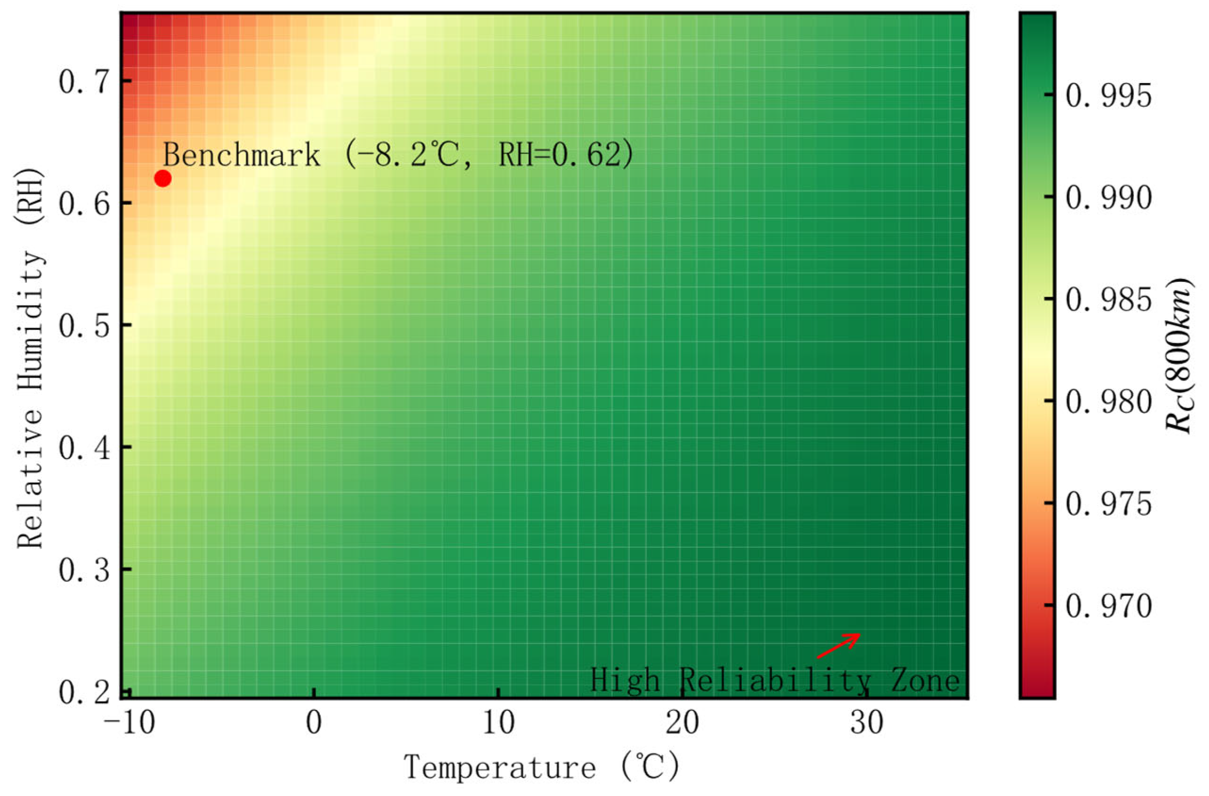
−10	3480.46	0.976	−0.2%
−8.2 (benchmark)	3595.68	0.978	0
0	4170.78	0.984	0.6%
15	5471.28	0.992	1.4%
35	7856.89	0.996	1.8%

and

Table 8. Humidity effects at fixed Temp = −8.2 °C.

RH	λC (km)	RC (800 km)	Reliability Variation Rate
0.20	5683.07	0.993	1.5%
0.35	4825.94	0.990	1.2%
0.50	4098.10	0.985	0.7%
0.62 (benchmark)	3595.68	0.978	0
0.75	3120.66	0.971	−0.7%

and Figure 11.

Table 7 shows temperature positively correlating with λ_C and R_C. Table 8 reveals humidity negatively affecting reliability. Figure 11 visualizes the joint impacts of temperature and humidity via a heatmap. The “high reliability zone” suggests that warm, dry environments optimize chassis reliability. Synthesizing the results of Table 7 and Table 8, within the temperature range of −10 °C~35 °C and RH range of 0.20~0.75, the maximum fluctuation of R_C (800 km) is less than 2%. In Figure 11, the green high reliability zone (R_C ≥ 0.985) covers nearly 75% of the environmental combinations. This response characteristic fully demonstrates the equipment’s relatively strong adaptability to environmental changes.

To further examine the robustness of reliability estimation, a sensitivity analysis on prior distributions is performed for subsystem C. Specifically, under the benchmark environmental state (Temp = 8.2 °C, RH = 0.62), the standard deviation (SD) of prior distributions for key parameters (θ_C, β_C, σ) is perturbed, and posterior estimates of R_C (800 km), including point estimates and 95% HPD intervals, are compared. The results are presented in

Table 9. Sensitivity analysis of R_C (800 km) to prior SD perturbations.

Prior SD Perturbation	${\widehat{\mathit{R}}}_{\mathit{C}}$ (800 km) Point Estimate	95% HPD Interval	Variation Rate of Interval Width
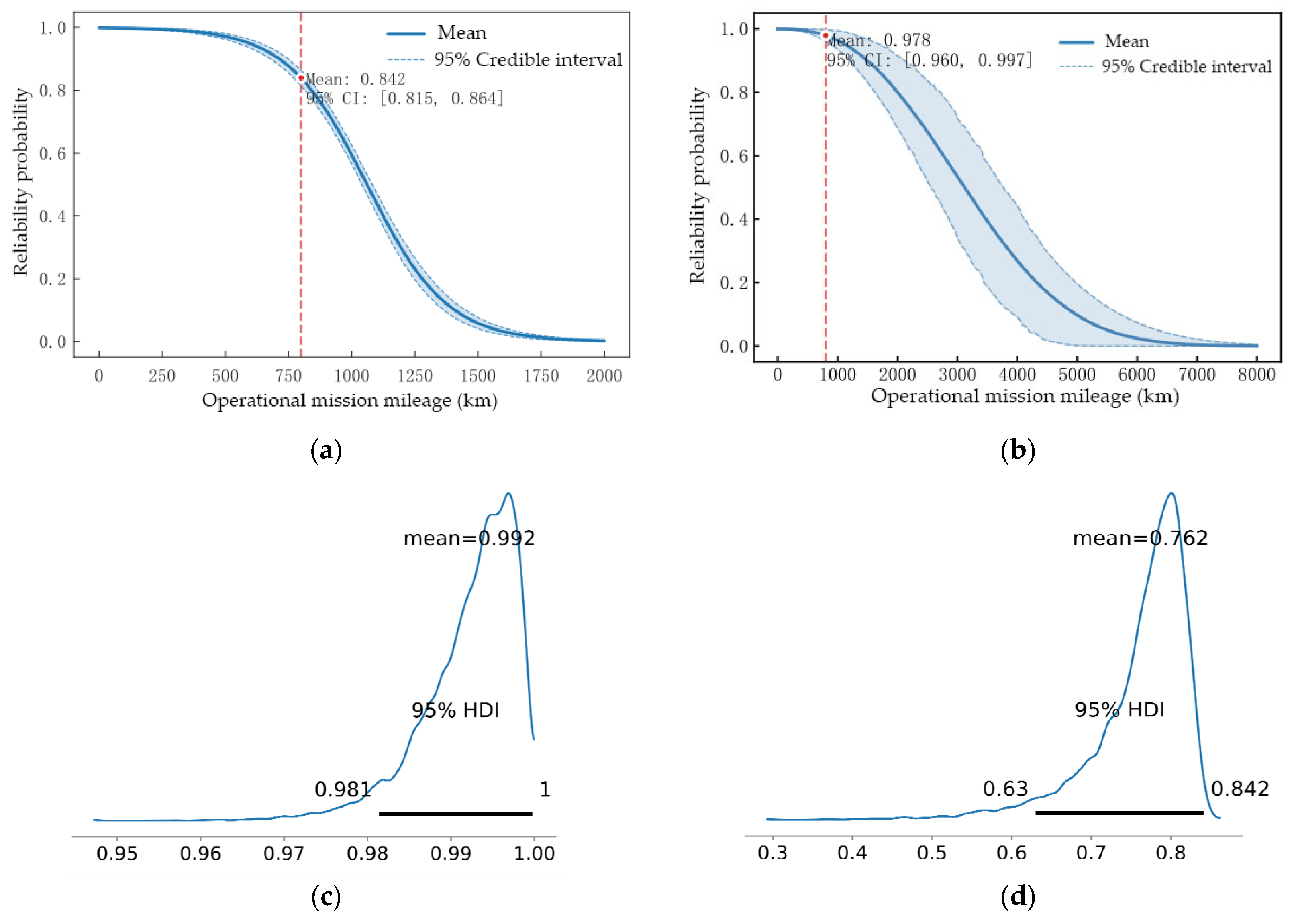
100 (benchmark)	0.978	[0.960, 0.997]	0
200	0.978	[0.959, 0.996]	0
50	0.979	[0.959, 0.997]	2.7%
10	0.978	[0.959, 0.997]	2.7%
5	0.979	[0.960, 0.997]	0
0.6	0.975	[0.953, 0.995]	13.5%
0.5	0.969	[0.942, 0.995]	43.2%

.

As shown in Table 9, when the prior SD falls within the range of 5~200, the point estimate and the 95% HPD interval for R_C (800 km) exhibit virtually no remarkable changes, showing only minor random fluctuations. This demonstrates strong stability in reliability assessment under moderately diffuse priors. In contrast, when the SD is narrowed to 0.6 and 0.5, the estimates become markedly distorted. The point estimate deviates significantly from the benchmark value, and the width of the HPD interval expands sharply. This indicates that overly restrictive priors (deviating from the “diffuse prior” assumption) introduce systematic bias into the posterior inference.

3.2.4. Comparative Validation

Explicitly integrating covariate effects into the Bayesian reliability assessment model is one of the contributions of this study. In this section, the proposed model (denoted as Model 1) is compared with two models using the field data of subsystem C. Diffuse priors are set uniformly for all parameters across the three models.

• Model 2: It assumes all chassis samples follow a single Weibull distribution and completely ignores the failure heterogeneity induced by covariates. The data model is Weibull (a, b), where a denotes the shape parameter and b represents the scale parameter. There is no covariate or grouping structure, and the failure law is characterized solely by global parameters.
• Model 3: It captures heterogeneity through data grouping. Specifically, historical data and operational test data are divided into two groups. It is assumed that two groups share the shape parameter a’, and the scale parameters follow a proportional relationship (the scale of historical data is ωb’, where b’ represents the scale of operational test data and ω is the proportional coefficient). The forms of the data models are Weibull (a’, b’) and Weibull (a’, ωb’).

The three models are evaluated in terms of goodness-of-fit and prediction accuracy. Figure 12 illustrates the comparison of empirical cumulative distribution functions (CDFs) among the three models. The red lines denote the CDFs of 100 sets of posterior predictive distributions. This figure is part of the posterior predictive check, which is used to visually demonstrate the goodness-of-fit. It can be seen that when TBF exceeds 6000 km, the gap between the blue line of Model 2 and the black line expands significantly compared to Model 1. Meanwhile, for Model 3, when TBF if less than approximately 3700 km, the gap between the blue line and the black line is relatively larger. This indicates that Model 1 demonstrates superior goodness-of-fit.

The ppp and widely applicable information criterion (WAIC) [34] are employed to quantify goodness-of-fit and predictive accuracy, respectively. WAIC is a pivotal tool for model selection within the Bayesian framework. Its core objective is to balance goodness-of-fit and its inherent complexity, thereby avoiding overfitting or underfitting issues. Mathematically, it essentially functions as an approximate estimation of predictive error based on the posterior distribution, and it can be interpreted in a simplified manner as $\mathrm{WAIC}=-2\times (\mathrm{lpd}-p_{waic})$, where lpd is the log pointwise predictive density, and $p_{waic}$ is the effective number of parameters. A quantitative comparison among the three models is presented in

Table 10. Quantitative comparison among the three models.

Model	WAIC	${\mathit{p}}_{\mathit{w}\mathit{a}\mathit{i}\mathit{c}}$	ppp
			Mean	Median	Lower Quartile	Upper Quartile
Model 1	845.172	4.111	0.535	0.386	0.423	0.647
Model 2	861.601	2.018	0.739	0.375	0.375	0.739
Model 3	865.938	2.987	0.597	0.357	0.469	0.601

.

From the data in Table 10, Model 1 exhibits the smallest WAIC value, indicating that its predictive accuracy is the best among the models. Meanwhile, Model 1 has the greatest $p_{waic}$ value, which is consistent with the actual scenario—it explicitly incorporates covariate effects, thus increasing the parameter count and leading to higher complexity. This also demonstrates that Model 1 translates the increased complexity into a gain in predictive accuracy.

In terms of goodness-of-fit, none of the ppp values of the models show extreme cases (values less than 0.05 or greater than 0.95), and all fall within a reasonable range. Model 1 performs the best in terms of mean and median, reflecting its relative advantage in goodness-of-fit. When comparing Model 3 and Model 2, the former has better goodness-of-fit but slightly lower predictive accuracy, which suggests that Model 3 has overfitting to some extent.

4. Conclusions

This study proposes a mission reliability assessment method for multi-phase data in operational testing. Taking the VMLS as a representative case study, a phased RBD is constructed considering the characteristics of mission subsystems and the types of test data. Customized reliability assessment models are developed for the distinct data features of different phases, and the assessment results from these models are consolidated to complete the mission reliability assessment of the system under test. The technical advantages and engineering applicability of the proposed method are validated through numerical case analyses based on a simulation experiment and a field deployment case. The main conclusions are as follows:

(1)

The construction of the phased RBD achieves a refined decomposition of the mission profile based on distinguishing mission subsystems and their corresponding test data types, laying a foundation for more rational mission reliability assessment.

(2)

The optimization model integrating maximum entropy principle with monotonic decreasing reliability constraint effectively reduces parameter estimation bias and suppresses estimation uncertainty.

(3)

The covariate-embedded Bayesian assessment model successfully combines heterogeneous historical data and operational testing data, while quantitatively characterizing the system’s adaptability to covariates.

(4)

The multi-path mission reliability assessment demonstrates that other performance metrics of the system also influence its mission reliability level, and its logic is extensible to other multi-phase systems (e.g., unmanned platforms, electronic warfare systems) with phased mission profiles and heterogeneous data sources.

The work presented in this paper provides a reference methodological framework for studying mission reliability assessment under operational testing conditions. Due to limitations in testing conditions, the covariate-embedded assessment models employed in this study have not yet incorporated additional unknown risk factors. The proposed framework exhibits inherent generalizability. Its core components, such as phased RBD construction, covariate-embedded Bayesian model, and multi-path synthesis, are adaptable to systems beyond VMLS. For instance, phased RBD can map to any equipment with sequential operational modes (e.g., reconnaissance–strike–assessment loops in UAVs), while covariate embedding accommodates diverse environmental drivers (e.g., jamming intensity in electronic warfare systems). The next phase of research will focus on validating this adaptability across domains.

References

- Sun, A.; Zhuang, Y.; Wang, B.; Bao, S.H.; Dong, L. Research and Application of Weapons and Equipments Combat Test; National Defense Industry Press: Beijing, China, 2021. [Google Scholar]
- Lu, P. Operational Test and Evaluation of US Marine Crops; National Defense Industry Press: Beijing, China, 2019. [Google Scholar]
- Cui, R.; Sun, J.; Yang, K.; Li, M. Construction method of operational test indicator systems based on UAF. Syst. Eng. Electron. 2025, 47, 1536–1550. [Google Scholar]
- Musallam, M.; Yin, C.; Bailey, C.; Johnson, M. Mission profile-based reliability design and real-time life consumption estimation in power electronics. IEEE Trans. Power Electron. 2014, 30, 2601–2613. [Google Scholar] [CrossRef]
- Lie, C.H.; Kuo, W.; Tillman, F.A.; Hwang, C. Mission effectiveness model for a system with several mission types. IEEE Trans. Reliab. 2009, 33, 346–352. [Google Scholar] [CrossRef]
- Zhang, R.; Mahadevan, S. Integration of computation and testing for reliability estimation. Reliab. Eng. Syst. Saf. 2001, 74, 13–21. [Google Scholar] [CrossRef]
- Li, S.; Wang, K.; Yuan, H.; Zhu, G.; Wang, X. An in-service mission reliability assessment method of complex equipment system. Air Space Def. 2023, 6, 23–28. [Google Scholar]
- Wang, S.; Zhang, S.; Li, Y.; Dong, Y.-S. Research on selective maintenance decision-making method of complex system considering imperfect maintenance. Acta Armamentarii 2018, 39, 1215–1224. [Google Scholar]
- Liu, Z.; Ma, X.; Hong, D.; Zhao, Y. Mission reliability assessment for battle-plane based on flight profile. J. Beijing Univ. Aeronaut. Astronaut. 2012, 38, 59–63. [Google Scholar]
- Lim, J.H.; Kim, S.Y. A Study on the Determination of Optimal Repair Parts Inventory based on Simulation and Analysis of Its Influencing Factors. Ind. Eng. Manag. Syst. 2024, 23, 515–534. [Google Scholar] [CrossRef]
- Guo, J.; Li, Y.; Peng, W.; Huang, H.-Z. Bayesian information fusion method for reliability analysis with failure-time data and degradation data. Qual. Reliab. Eng. Int. 2022, 38, 1944–1956. [Google Scholar] [CrossRef]
- Hu, J.; Huang, H.; Li, Y.; Gao, H. Bayesian prior information fusion for power law process via evidence theory. Commun. Stat.-Theory Methods 2022, 51, 4921–4939. [Google Scholar] [CrossRef]
- Kleyner, A.; Bhagath, S.; Gasparini, M.; Robinson, J. Bayesian techniques to reduce the sample size in automotive electronics attribute testing. Microelectron. Reliab. 1997, 37, 879–883. [Google Scholar] [CrossRef]
- Steiner, S.; Dickinson, R.M.; Freeman, L.J.; Simpson, B.A.; Wilson, A.G. Statistical methods for combining information: Stryker family of vehicles reliability case study. J. Qual. Technol. 2015, 47, 400–415. [Google Scholar] [CrossRef]
- Gilman, J.F.; Fronczyk, K.M.; Wilson, A.G. Bayesian modeling and test planning for multiphase reliability assessment. Qual. Reliab. Eng. Int. 2019, 35, 750–760. [Google Scholar] [CrossRef]
- Dewald, S.L.; Holcomb, R.; Parry, S.; Wilson, A. A Bayesian approach to evaluation of operational testing of land warfare systems. Mil. Oper. Res. 2016, 21, 23–32. [Google Scholar]
- Krolo, A.; Bertsche, B. An approach for the advanced planning of a reliability demonstration test based on a Bayes procedure. In Proceedings of the Annual Reliability and Maintainability Symposium, Tampa, FL, USA, 27–30 January 2003; pp. 288–294. [Google Scholar]
- Tait, N.R.S. Robert Lusser and Lusser’s Law. Saf. Reliab. 1995, 15, 15–18. [Google Scholar] [CrossRef]
- Martz, H.F.; Waller, R.A. 14. Bayesian methods. Methods Exp. Phys. 1994, 28, 403–432. [Google Scholar]
- Flegal, J.M.; Jones, G.L. Implementing MCMC: Estimating with confidence. In Handbook of Markov Chain Monte Carlo; Chapman and Hall/CRC: Boca Raton, FL, USA, 2011; Volume 1, pp. 175–197. [Google Scholar]
- Jerke, G.; Kahng, A.B. Mission profile aware IC design—A case study. In Proceedings of the 2014 Design, Automation & Test in Europe Conference & Exhibition (DATE), Dresden, Germany, 24–28 March 2014; IEEE: Piscataway, NJ, USA, 2014; pp. 1–6. [Google Scholar]
- Franciosi, C.; Polenghi, A.; Lezoche, M.; Voisin, A.; Roda, I.; Macchi, M. Semantic interoperability in industrial maintenance-related applications: Multiple ontologies integration towards a unified BFO-compliant taxonomy. In Proceedings of the 16th IFAC/IFIP International Workshop on Enterprise Integration, Interoperability and Networking, EI2N, Valletta, Malta, 24–26 October 2022; SCITEPRESS-Science and Technology Publications: Setúbal, Portugal, 2022; pp. 218–229. [Google Scholar]
- Xia, X.; Ye, L.; Li, Y.; Chang, Z. Reliability evaluation based on hierarchical bootstrap maximum entropy method. Acta Armamentarii 2016, 37, 1317–1329. [Google Scholar]
- Guo, J.; Wilson, A. Bayesian methods for estimating system reliability using heterogeneous multilevel information. Technometrics 2013, 55, 461–472. [Google Scholar] [CrossRef]
- Zhang, W.; Yang, H.; Zhang, S.H. Reliability assessment for device with only safe-or-failure pattern based on Bayesian hyprid prior approach. Acta Armamentarii 2016, 37, 505–511. [Google Scholar]
- Karras, C.; Karras, A.; Avlonitis, M.; Sioutas, S. An overview of mcmc methods: From theory to applications. Proceedings of the IFIP International Conference on Artificial Intelligence Applications and Innovations, Crete, Greece, 17–20 June 2022, Springer International Publishing: Cham, Switzerland, 2022; 319–332. [Google Scholar]
- Wikle, C.K. Hierarchical Bayesian models for predicting the spread of ecological processes. Ecology 2003, 84, 1382–1394. [Google Scholar] [CrossRef]
- Bian, R.; Zhang, Y.; Pan, Z.; Cheng, Z.; Bai, S. Reliability analysis of phased-mission system of systems for escort formation based on BDD. Acta Armamentarii 2020, 41, 1016–1024. [Google Scholar]
- Chen, J. Survival Analysis and Reliability; Peking University Press: Beijing, China, 2005. [Google Scholar]
- Jia, X.; Guo, B. Reliability evaluation for products by fusing expert knowledge and lifetime data. Control Decis. 2022, 37, 2600–2608. [Google Scholar]
- Hoffman, M.D.; Gelman, A. The No-U-Turn sampler: Adaptively setting path lengths in Hamiltonian Monte Carlo. J. Mach. Learn. Res. 2014, 15, 1593–1623. [Google Scholar]
- Turkkan, N.; Pham-Gia, T. Computation of the highest posterior density interval in Bayesian analysis. J. Stat. Comput. Simul. 1993, 44, 243–250. [Google Scholar] [CrossRef]
- Dahl, F.A. On the conservativeness of posterior predictive p-values. Stat. Probab. Lett. 2006, 76, 1170–1174. [Google Scholar] [CrossRef]
- Vehtari, A.; Gelman, A.; Gabry, J. Practical Bayesian model evaluation using leave-one-out cross-validation and WAIC. Stat. Comput. 2017, 27, 1413–1432. [Google Scholar] [CrossRef]