Abstract
Multicollinearity in logistic regression models can result in inflated variances and yield unreliable estimates of parameters. Ridge regression, a regularized estimation technique, is frequently employed to address this issue. This study conducts a comparative evaluation of the performance of 23 established ridge regression estimators alongside Logistic Regression, Elastic-Net, Lasso, and Generalized Ridge Regression (GRR), considering various levels of multicollinearity within the context of logistic regression settings. Simulated datasets with high correlations (0.80, 0.90, 0.95, and 0.99) and real-world data (municipal and cancer remission) were analyzed. Both results show that ridge estimators, such as , and , exhibit strong performance in terms of Mean Squared Error (MSE) and accuracy, particularly in smaller samples, while GRR demonstrates superior performance in large samples. Real-world data further confirm that GRR achieves the lowest MSE in highly collinear municipal data, while ridge estimators and GRR help prevent overfitting in small-sample cancer remission data. The results underscore the efficacy of ridge estimators and GRR in handling multicollinearity, offering reliable alternatives to traditional regression techniques, especially for datasets with high correlations and varying sample sizes.
1. Introduction
Logistic regression stands as a key method in statistical modeling, particularly for binary classification, where the outcome variable is dichotomous. Its widespread use in various fields, including epidemiology, social sciences, and machine learning, is due to its ability to model the probability of an event occurring as a function of one or more predictor variables [1]. Unlike a linear model, which assumes a continuous outcome, logistic regression uses a logistic function to convert the linear combination of predictors into a probability, making it well-suited for categorical outcomes. This ability to estimate probabilities directly makes logistic regression invaluable for risk assessment, predictive modeling, and hypothesis testing in several applied contexts.
However, multicollinearity, characterized by a high correlation among predictor variables, adds complexity to the interpretation and reliability of logistic regression models [2]. Although multicollinearity does not introduce bias into the coefficient estimates in the same manner as in linear regression, it significantly inflates the standard errors of these coefficients [3]. Inflated standard errors lead to decreased t-statistics (or Wald statistics) associated with the coefficients, which reduces the likelihood of detecting statistically significant effects. This increases the risk of Type II errors, where genuine relationships between predictors and the outcome may be overlooked [4]. As a result, the practical implications of multicollinearity can lead to misleading conclusions, ultimately compromising the model’s usefulness for both predictive and explanatory purposes. Although the coefficients are not biased, their stability diminishes, resulting in substantial changes in the estimated coefficients when there are slight variations in the data. This instability makes it challenging to determine the true magnitude and direction of the predictors’ effects [5]. Multicollinearity also complicates the assessment of variable importance. The high correlation among predictors complicates the identification of their individual impacts on the outcome, risking misleading conclusions about their influence [6]. The interpretation of odds ratios, which are central to logistic regression, can also be problematic. With inflated standard errors, the confidence intervals around the odds ratios broaden, making it difficult to draw precise inferences about the magnitude of the effects. This complicates the practical application of the model findings [7].
To mitigate multicollinearity in logistic regression, researchers often use regularization techniques like Ridge Regression, Lasso, and Elastic Net [8]. These methods are intended to minimize the overlap between predictor variables, strengthen the consistency of coefficient estimates, and boost the overall reliability and clarity of the model.
Hoerl and Kennard (1970) introduced ridge regression to address multicollinearity in engineering data. Their work showed that a nonzero ridge parameter (k) can lower the MSE of ridge regression compared to the variance of the Ordinary Least Squares (OLS) estimator [9]. Since their pioneering contribution, extensive research has been conducted to refine and enhance the ridge regression methodologies. A multitude of scholars have proposed innovative estimators for the ridge parameter, making remarkable strides in the field. Their contributions not only enrich existing knowledge but also open new avenues for exploration and understanding. Notable contributions include those of McDonald & Schwing, 1973; Hoerl et al., 1975; McDonald & Galarneau, 1975; J. F. & P, 1976; Dempster et al., 1977; Gibbons, 1981; Schaeffer et al., 1984; Schaeffer, 1986; Walker & Birch, 1988; Kibria, 2003; Khalaf & Shukur, 2005 [10,11,12,13,14,15,16,17,18,19,20] and very recently Muniz & Kibria, 2009; Månsson et al., 2010; Kibria et al., 2012; Hefnawy & Farag, 2014; Aslam, 2014; A. V. Dorugade, 2014; Arashi & Valizadeh, 2015; Ayinde & Lukman, 2016; Lukman & Ayindez, 2017; Melkumova & Shatskikh, 2017; Lukman et al., 2018, 2019; Herawati et al., 2018, 2024; Yüzbaşı et al., 2020; Golam Kibria & Lukman, 2020; Kibria, 2023; Hoque & Kibria, 2023; Mermi et al., 2024; Nayem et al., 2024; Hoque & Kibria, 2024; Yasmin & Kibria, 2025, among others [20,21,22,23,24,25,26,27,28,29,30,31,32,33,34,35,36,37,38,39,40]. These contributions have played a critical role in the ongoing refinement of ridge regression techniques, ensuring their continued relevance in statistical modeling and analyses.
Despite extensive research on ridge regression, relatively little attention has been devoted to its application in logistic regression. Schaeffer et al. (1984) presented a logistic ridge regression (LRR) estimator, and later research investigated different approaches for estimating the ridge parameter (k) and evaluated their effectiveness using Monte Carlo simulations [16,17,23]. Recently, Mermi et al. (2024) carried out a thorough comparative evaluation of 366 ridge parameter estimators introduced over various periods, taking into account elements like the number of independent variables, sample size, correlation among predictors, and variance of errors [38]. In the present study, we incorporated 16 of the most effective estimators from Mermi et al. (2024). Furthermore, we utilized seven estimators that Kibria and Lukman (2020) and Kibria (2023) specifically suggested for non-normal population distributions, guaranteeing a thorough assessment of logistic ridge regression across different modeling scenarios [34,36].
In the presence of multicollinearity, selecting an optimal estimator requires a careful balance between minimizing the MSE and maximizing the classification accuracy. MSE minimization is crucial for obtaining precise parameter estimates and reducing prediction errors, particularly in regression contexts, where deviations from true values carry significant implications [5]. However, an exclusive focus on the MSE may fail to account for the importance of classification accuracy, especially in binary or categorical response settings, where correct classification is critical for decision-making [7]. The selection of an estimator must strategically weigh these competing metrics, emphasizing MSE reduction in scenarios where precise numerical predictions are paramount and prioritizing classification accuracy when robust categorical predictions are the primary objective. As evidenced by numerous simulation studies, the optimal estimator is often context-dependent, varying based on the specific application and the relative costs associated with prediction errors versus misclassifications. Unlike much of the existing literature that focuses predominantly on linear models or limits evaluation to MSE, this study emphasizes both MSE and classification accuracy to provide a more comprehensive assessment of the model performance in the presence of multicollinearity. While previous studies have explored various ridge estimators in linear regression contexts, there remains a significant gap in systematically evaluating their effectiveness within logistic regression frameworks, particularly under high multicollinearity and non-normal data conditions. By incorporating recently developed and robust ridge parameter estimators tailored for such scenarios, this study aims to address this gap and offer practical guidance for the selection of estimators in binary classification problems. Therefore, it is crucial to conduct a thorough assessment of both the MSE and classification accuracy to make a well-informed choice concerning estimator selection when multicollinearity is present.
This research intends to conduct an in-depth comparison of 23 ridge regression estimators alongside traditional LR, Lasso, EN, and GRR. This examination goes beyond the typical emphasis on MSE by also assessing classification accuracy in situations of multicollinearity. The objective of this study is to enhance the existing literature on ridge regression by systematically evaluating the performance of estimators under various levels of multicollinearity. Additionally, real-world datasets will be utilized to corroborate the findings obtained from simulations, thereby demonstrating the practical applicability of the methodologies employed.
2. Methodology
The OLS estimator of is the following:
In regression analysis, let Y be the response, X be a matrix of predictors, and θ be a parameter vector. The ε denotes the random error. When the response variable is binary, standard OLS regression is no longer suitable, and logistic regression is employed instead. In this section, we present LRR, initially proposed by Schaefer et al. (1984), and explore its enhancements through more recent advancements [16]. The refinements aim to enhance the performance and stability of logistic ridge regression, making it a more robust alternative in cases of multicollinearity.
Let the th observation of the response, , follows a Bernoulli distribution, denoted as , where represents the probability of success associated with the th observation. The parameter is modeled as a function of the predictors using the logit link, ensuring that predicted probabilities remain within the unit interval.
where is the data matrix with predictors, and is the coefficients vector. The approach of maximum likelihood for estimating involves maximizing the subsequent log-likelihood.
This can be achieved by setting the first derivative of the expression equal to zero. As a result, the maximum likelihood estimates are found by solving the resulting equation:
As this equation is nonlinear in nature, the Newton-Raphson method must be employed to find a solution. As a result, the solution to the previously mentioned equation can be obtained through the subsequent iterative weighted least squares method.
where , and
The asymptotic covariance matrix of the maximum likelihood estimator is the inverse of the matrix of second derivatives:
and the asymptotic MSE equals:
where is the eigenvalue of matrix. A key drawback of the maximum likelihood estimate is that its asymptotic variance can inflate due to high correlation among independent variables, leading to small eigenvalues. To address this multicollinearity issue, Schaefer et al. (1984) proposed using the following LRR estimator [16]:
Numerous ridge estimators have been suggested in the literature for different kinds of models, as mentioned previously, to determine the ridge parameter k. For this study, we selected the 16 most effective estimators identified by Mermi et al. (2024) based on their performance in different statistical settings [38]. In addition, we incorporated seven estimators introduced by Kibria & Lukman (2020) and Kibria (2023) which are specifically designed for asymmetric data [34,36]. These 23 estimators were selected to ensure a comprehensive comparison that spanned both classical and modern approaches to ridge parameter selection. Including estimators suited for asymmetric data is particularly important because such data structures frequently arise in applied settings and can adversely affect the performance of conventional ridge estimators [9,19]. The comprehensive set of 23 ridge estimators utilized in this study, encompassing both simulation-based analyses and real-life applications, is systematically presented in Table 1.

Table 1.
Ridge penalties compared in this study.
2.1. Generalized Ridge Regression (GRR)
In 2017, Yang and Emura presented a GRR estimator that uses non-uniform shrinkage instead of the conventional uniform shrinkage method, replacing the identity matrix with a diagonal matrix [44].
For a binary response variable , the GRR estimator can be adapted by incorporating it into the penalized logistic regression framework. The parameter estimates are derived by minimizing the penalized negative log-likelihood, as follows:
where is the predicted probability from logistic regression, is the shrinkage parameter, is the threshold parameter, and is a diagonal matrix encoding non-uniform penalties for each coefficient [45].
where is a standardized initial estimate of , , and serves as an initial estimator based on a simple componentwise pseudo-regression.
This formulation allows for adaptive shrinkage, where coefficients associated with stronger initial signals (larger ) are penalized less, while weaker signals are shrunk more aggressively, thus promoting both interpretability and generalization in high-dimensional binary classification problems.
2.2. Least Absolute Shrinkage and Selection Operator (Lasso)
Lasso (Tibshirani, 1996) is an effective regression method that conducts variable selection and regularization at the same time, enhancing both the precision and clarity of statistical models [46]. Unlike ridge regression, which uses the squared norm, Lasso employs the norm to reduce the total of squared differences while adhering to a limitation on the overall absolute size of the coefficients. This constraint promotes sparsity in the model, effectively mitigating multicollinearity and identifying a subset of truly relevant predictors [46,47].
where is the log-likelihood of the binary logistic model, is the tuning (regularization) parameter, is the coefficient vector, is the norm to shrink coefficients toward zero, n is the sample size, and p is the number of predictors.
2.3. Elastic Net (EN)
The EN, which was introduced by Zou and Hastie in 2005, extends Lasso by combining penalties from both the norm (Lasso) and norm (ridge), addressing limitations in variable selection [48]. This dual regularization reduces coefficients like ridge regression while enforcing sparsity by setting some to zero, as in the case of Lasso. The norm ensures model sparsity, while the norm alleviates restrictions on the number of selected predictors, enabling more flexibility [49]. EN’s ability to select more predictors than Lasso makes it a powerful tool for variable identification, as demonstrated in spectral data analysis [50]. For a binary outcome variable, the EN reduces the penalized negative log-likelihood of the logistic regression model to calculate the best-parameter vector.
Let:
Then the EN estimator becomes:
where is the predicted probability that , is the coefficient vector, is the regularization strength, and is the weight between the norm and norm ( Ridge, Lasso.
In this study for GRR, Lasso, and EN, the optimum , tuning parameter was obtained using 5-fold cross-validation.
2.4. Simulation Study
The objective of this research is to evaluate the effectiveness of the leading ridge estimators against LR, Lasso, EN, and GRR, focusing on minimizing MSE and enhancing accuracy. Due to the infeasibility of a theoretical comparison, a Monte Carlo simulation study has been performed utilizing the R programming language [51]. The method used for generating data for the models adheres to a recognized procedure [19].
where indicates the correlation between two predictors, denotes the independent pseudo-random variable, and P indicates the number of independent variables. Moreover, the response, was obtained through the Bernoulli distribution, where:
In the modeling process, we considered three distinct values for the number of independent variables (, and 10), the correlation between the predictors (, and 0.99), and three sample sizes (, and 300). The procedure for generating data for the predictors was carried out according to the established values of P, and n. In order to confirm the reliability of the findings, the experiment was conducted 5000 times.
Following the theoretical foundation established by Newhouse and Oman (1971), which posits that the MSE is minimized when the coefficient vector aligns with the normalized eigenvector corresponding to the largest eigenvalue of the matrix, the simulation study computes MSE by comparing estimated coefficient vectors, , derived from various models, to the true [52]. This true is determined for each simulation by extracting and normalizing the eigenvector associated with the largest eigenvalue of , ensuring , thereby providing a theoretically grounded benchmark for evaluating estimator performance through the calculation of the average squared difference between and . The average estimated MSE was computed using the formula applied to all simulations [39].
where is the estimators, is the parameter, and N = 5000.
In the evaluation of the classification performance, accuracy was used as a key metric to quantify the proportion of correctly predicted binary outcomes. For each simulation, we applied a 70% training and testing split on the simulated data. Models were trained on the training subset, and predictions were generated for the held-out test set. The predicted values, which were initially probabilities derived from the logistic regression link function, were converted into binary classifications using a threshold of 0.5. Specifically, if the predicted probability exceeded 0.5, the observation was classified as 1; otherwise, it was classified as 0.
The models’ overall accuracy was calculated using a confusion matrix based on the total number of correctly classified observations [53].
where TP—true positive, TN—negative, FP—false positive, and FN—false negative, accuracy serves as the comprehensive metric for the model’s ability to make correct predictions across the entire dataset. For each simulation, accuracy values were calculated, and the average accuracy was then computed across all simulations, considering different combinations of parameters (n, P, and ) and models.
3. Results & Discussion
In this part, we carried out an extensive simulation study to assess the effectiveness of ridge estimators relative to conventional logistic regression, elastic net, Lasso, and generalized ridge regression. The results, summarized in Table 2, Table 3, Table 4 and Table 5, present the MSE and classification accuracy of the estimators under different conditions. Specifically, this study examines the impact of correlation coefficients (0.80, 0.90, 0.95, and 0.99). The findings, systematically detailed in these tables, illustrate the effects of different correlation structures, the number of independent variables, and sample sizes on the estimator performance.
Table 2.
Estimated MSE values and Accuracy for correlation 0.80.
Table 3.
Estimated MSE values and Accuracy for correlation 0.90.
Table 4.
Estimated MSE values & Accuracy for correlation 0.95.
Table 5.
Estimated MSE values & Accuracy for correlation 0.99.
Table 2 compares the MSE and Accuracy across various regression models under moderate multicollinearity (correlation = 0.80) for different predictor counts (P = 3, 5, 10) and sample sizes (n = 100, 200, 300). For P = 3, consistently achieves the lowest MSE (0.088), demonstrating its effectiveness in low-dimensional settings. As P increases to 5, remains optimal, with an MSE of 0.082. However, for P = 10, GRR performs best, with an MSE of 0.064 at n = 300, highlighting its capacity for high-dimensional data. LR exhibits the highest MSE, indicating limitations in multicollinear environments. EN and Lasso show competitive performance, especially with larger P and n, benefiting from regularization.
In terms of accuracy, most models show stable performance, with slight improvements as sample size increases. For P = 3, ridge estimators like , , and maintain an accuracy of 0.736 at n = 100, rising to 0.738 at n = 300. With P = 5, models such as GRR, EN, and Lasso achieve accuracies of 0.764 to 0.766 at n = 300, demonstrating effectiveness in moderate complexity. For P = 10, GRR leads with an accuracy of 0.812 at n = 300, showing its robustness in high-dimensional spaces.
Table 3 shows that under high multicollinearity (correlation = 0.90), MSE values increase, indicating greater prediction difficulty. Focusing on the non-penalized methods first, we see that LR exhibits the highest MSE, particularly as increases, indicating its vulnerability to overfitting with more predictors. GRR substantially reduces MSE compared to LR, highlighting the benefits of regularization. As expected, increasing sample size () generally decreases MSE for all methods, as more data provides a better estimate of the underlying relationships. For the ridge estimators, we observe generally low and stable MSE across different and , suggesting that these methods are less sensitive to the increase in predictor dimension in this context. However, some estimators like , and show relatively higher MSE compared to others, indicating potential challenges in capturing the underlying data structure with specific kernels. Notably, , and achieve some of the lowest MSE values, suggesting good performance in this scenario.
Regarding accuracy, the table displays the proportion of correctly classified instances for each estimator under the same conditions. Like the MSE trends, the accuracy tends to improve with increasing sample size () for most methods, reflecting the benefit of more data. LR, which suffered from a high MSE, also exhibits the lowest accuracy, reinforcing the detrimental effect of overfitting. In contrast, the penalized methods, Lasso and EN, demonstrate higher accuracy, with GRR achieving the highest accuracy among the estimators. The ridge estimators, except for , and , achieve high and relatively consistent accuracy across different and , often surpassing the traditional methods. This suggests that the ridge estimators are effective in capturing the non-linear relationships in the data, leading to better classification performance. The methods , and , which had low MSE, also maintain high accuracy, further indicating their effectiveness. The methods , , and that showed relatively higher MSE also show lower accuracy compared to other ridge estimators, suggesting a link between MSE and classification performance.
Table 4 presents the MSE for various estimators across different parameter settings (P = 3, 5, 10) and sample sizes (n = 100, 200, 300) given a correlation of 0.95. Firstly, within the ridge estimators, we observe a general trend of decreasing MSE as the sample size (n) increases, as expected due to the larger amount of information available for estimation. Notably, the estimators ,and consistently demonstrate lower MSE values, particularly as P increases, suggesting superior performance in capturing the underlying relationship under higher dimensionality. In contrast, the estimator exhibits significantly higher MSE, indicating poor performance and potential instability. Among the traditional methods, GRR consistently achieves the lowest MSE across all settings, highlighting its effectiveness in handling high correlations and varying dimensions. EN and Lasso also demonstrate reasonable performance, with the MSE decreasing as the sample size increases, albeit not as effectively as the GRR. LR shows the highest MSE, especially with larger P values, indicating its sensitivity to high correlation and dimensionality.
The accuracy metric presented alongside the MSE provides insights into the classification performance of the estimators. Similar to the MSE trends, we observe that the accuracy generally improves with increasing sample size across all estimators. However, the ridge estimators show remarkably consistent and high accuracy, often reaching 83.7% for P = 10 and n = 300. This suggests that these estimators are robust and effective in capturing underlying patterns, even with increased dimensionality. GRR, EN, and Lasso also exhibit good accuracy, with GRR showing slightly better performance, especially at higher P values. LR, while showing improvement with larger sample sizes, lags the other methods in terms of accuracy, consistent with its higher MSE.
Table 5 reveals the impact of extremely high multicollinearity (correlation of 0.99) on the MSE. The near-perfect correlation increases the MSE values across all models, highlighting the difficulty of accurate prediction under extreme dependencies. The ridge estimators, particularly ,and consistently exhibit the lowest MSE across all parameter settings (P = 3, 5, 10) and sample sizes. Importantly, their MSE values decrease as the sample size increases, demonstrating the desired consistency and effectiveness in handling the strong dependencies. In contrast, the estimator shows significantly higher MSE, indicating poor performance and a lack of robustness to high correlation. Among the classical methods, GRR stands out with the lowest MSE and exhibits a clear trend of decreasing MSE with increasing sample size, suggesting a superior ability to mitigate the impact of high correlation. EN and Lasso also show reasonable performance, with MSE decreasing as the sample size increases, although not as effectively as GRR. LR exhibits the highest MSE, especially with larger P values, and shows less consistent improvement with increasing sample size, indicating its struggle to handle the strong linear dependency of the data.
From Table 5, we observe that the accuracy generally improves with increasing sample size across all estimators. The ridge estimators, specifically ,and , demonstrate remarkably consistent and high accuracy, often reaching 84.3% for P = 10 and n = 300. This suggests that these estimators are robust and effective in capturing the underlying patterns, even with extreme correlations. GRR also exhibits good accuracy, showing slightly better performance, especially at higher P values. EN and Lasso show comparable accuracy to GRR, while LR lags the other methods in terms of accuracy, consistent with its higher MSE.
4. Applications
We conducted an analysis of two real-life datasets to effectively illustrate the findings derived from the simulation presented in this section.
4.1. Municipal Data
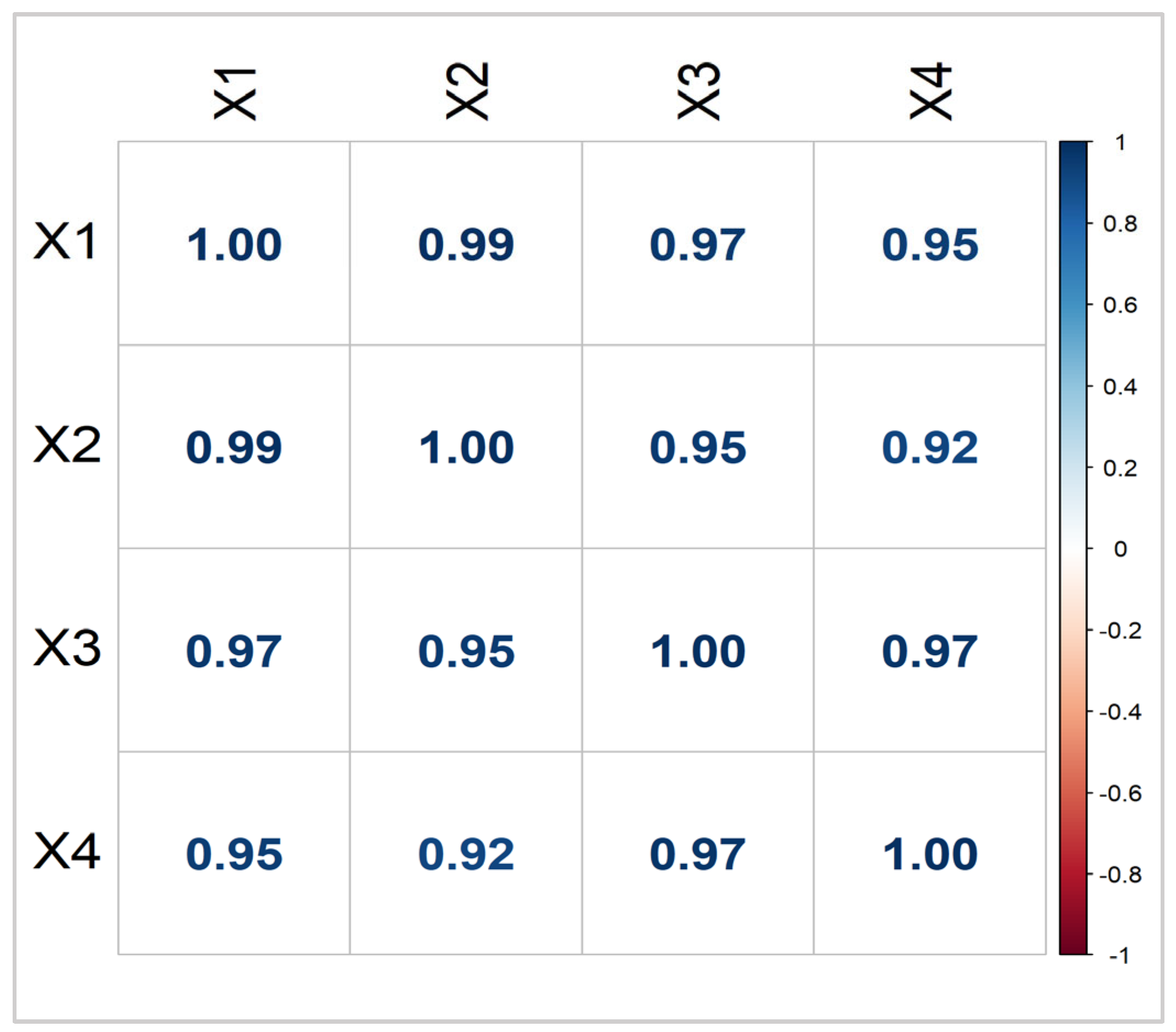
In this part, the models are applied to the municipal dataset from Statistics Sweden [54]. A binary logistic regression model is employed, with the dependent variable indicating whether the net population expands (coded as 1) or contracts (coded as 0). The model aims to explain the response variable using the following predictors: X1 (population), X2 (number of unemployed individuals), X3 (number of newly constructed buildings), and X4 (number of bankrupt firms).
The full dataset consists of 271 entries, which correspond to the municipalities in Sweden. The correlation plot illustrated in Figure 1 indicates that all correlation values are above 0.90, with some approaching 0.99. Furthermore, the condition number is 38.33, suggesting a notable issue with multicollinearity within the data [55].

Figure 1.
Correlation matrix of municipal data.
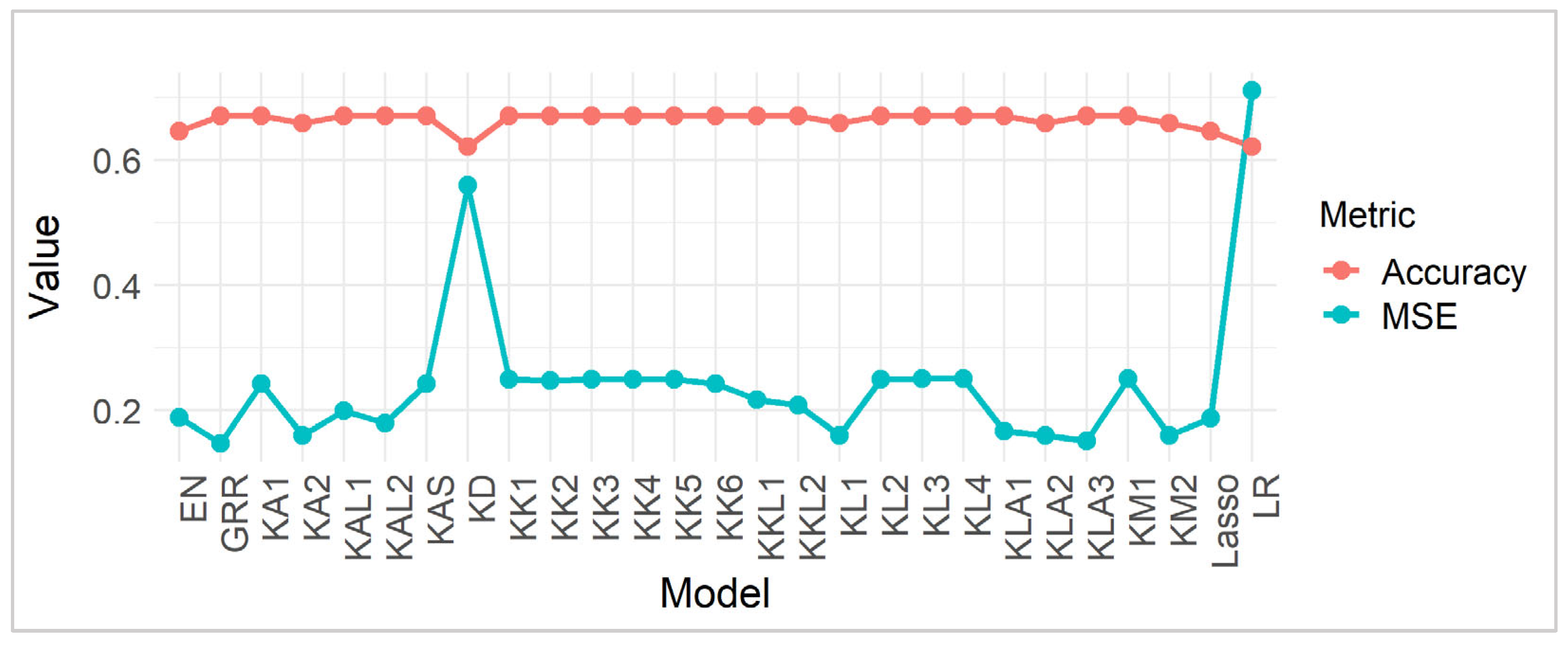
Table 6 presents the performance of various statistical estimators, primarily focusing on shrinkage methods, evaluated based on MSE and Accuracy. Lower MSE values indicate a closer approximation of the estimated values to the true values, suggesting higher precision and a reduced prediction error. Conversely, higher accuracy scores reflect a greater proportion of correct predictions, implying a better classification performance. Examining the estimators, we observe that GRR exhibits the lowest MSE (0.1470747), indicating superior precision among the tested models, which aligns with the simulation results since this is a large sample. This suggests that the GRR, by introducing a form of regularization that shrinks coefficients towards zero, effectively mitigates overfitting and improves the model’s predictive accuracy. In contrast, LR, without any shrinkage, shows the highest MSE (0.7111922), highlighting the potential for substantial prediction errors in unregularized models, especially in datasets with multicollinearity or high dimensionality. The Lasso and EN estimators, which also incorporate regularization, fall within a moderate range of MSE values, demonstrating their ability to balance bias and variance, although not as effectively as GRR for this data (Figure 2).
Table 6.
Comparison of MSE and Accuracy for municipal data.

Figure 2.
MSE and Accuracy comparison.
In terms of accuracy, most of the estimators, including GRR and the various ridge estimators, such as , , and achieve an accuracy of approximately 67.1%, suggesting a consistent ability to correctly classify a significant portion of the observations. This uniform accuracy across several shrinkage estimators implies that, while the MSE varies significantly, the overall classification performance remains relatively stable. However, the LR estimator exhibits a lower accuracy of 62.2%, aligning with its higher MSE and indicating a less reliable classification capability. The Lasso and EN estimators, like their MSE results, show moderate accuracy levels (64.63%), further demonstrating their balanced performance. The consistency of high accuracy among the ridge estimators, despite variations in their specific shrinkage parameters, suggests that these methods are robust in classification tasks, potentially due to their specific adaptations to the dataset’s characteristics. Overall, the findings suggest that shrinkage methods, particularly GRR, are effective in minimizing prediction errors and maintaining high classification accuracy for large data, highlighting the importance of regularization in statistical modeling.
4.2. Cancer Remission Data
In contrast to the previous analysis, which examined a larger dataset of approximately 271 samples, we now focus on a smaller dataset to further evaluate the performance of the estimators. Specifically, we analyze the Cancer Remission dataset [56,57], which consists of 27 observations. This dataset provides a valuable opportunity to assess the performance of estimators in a setting with a limited sample size, offering insights into their robustness and effectiveness in small-sample scenarios. The response variable is binary, indicating whether a patient achieves complete cancer remission (Y = 1) or not (Y = 0). The dataset includes observations from 27 patients, of whom nine experienced complete remission. The explanatory variables in the dataset are standardized such that corresponds to a correlation matrix.
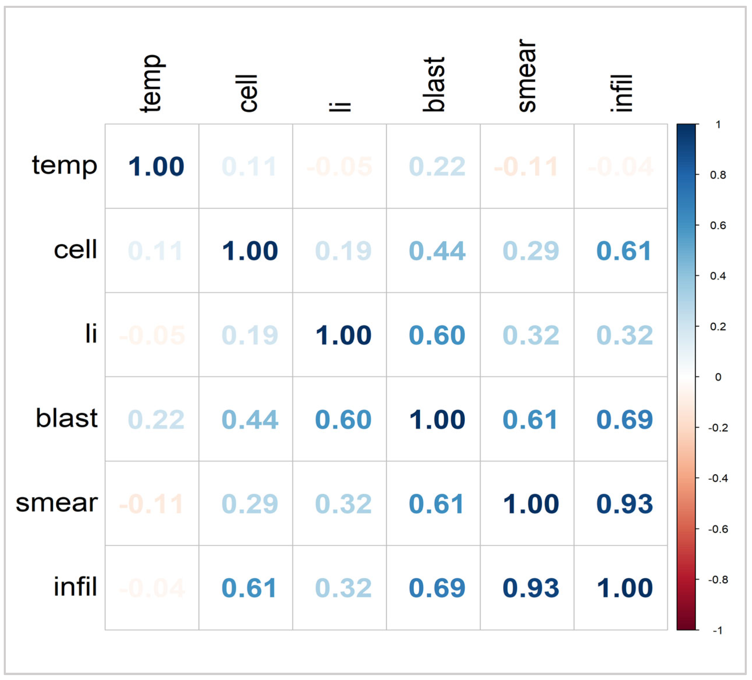
The condition number computed as . This high condition number and Figure 3 strongly suggest the presence of severe multicollinearity, which can adversely impact the stability and reliability of parameter estimates in regression models [55].
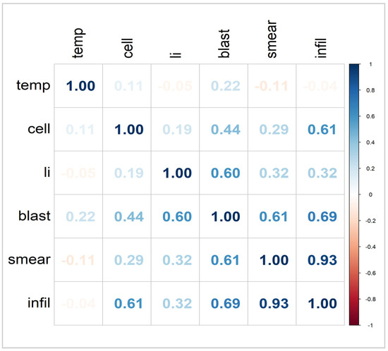
Figure 3.
Correlation matrix of cancer remission data.
Table 7 presents the MSE and accuracy for various models, including ridge regression with different shrinkage estimators, LR, Lasso, EN, and GRR. Several models, particularly those with high MSE values like LR, Lasso, EN, and some ridge estimators, achieve perfect accuracy (100%). However, with a sample size of only 27, this perfect accuracy strongly suggests overfitting. Overfitting occurs when a model conforms too closely to the training data, picking up noise instead of true patterns, which results in weak performance on new, unseen data. The models with lower MSE values, such as , , and , while not achieving perfect accuracy, might offer a more robust representation of the underlying relationships in the data, as they are less prone to overfitting.
Table 7.
Comparison of MSE and Accuracy for cancer remission data.
5. Concluding Remarks
This study aims to evaluate the effectiveness of ridge regression, GRR, Lasso, and Elastic Net within the context of a logistic regression model by balancing the MSE with prediction accuracy. Given that a theoretical assessment of the estimators cannot be performed, a comprehensive simulation study has been carried out to assess their performance across various parametric conditions. The simulation studies, focusing on varying levels of correlation (0.80, 0.90, 0.95, and 0.99), consistently demonstrate the superior performance of ridge estimators with varying penalties, particularly , and , for small samples and GRR for large samples in terms of both MSE and accuracy. These methods exhibit desirable characteristics, such as lower MSE, indicating a better fit and consistent reduction of MSE with increasing sample size, highlighting robustness. Furthermore, they achieve high accuracy, suggesting reliable prediction capabilities even under severe multicollinearity. The simulation findings are corroborated by the real-world applications involving municipal and cancer remission data. Specifically, in the municipal data, characterized by high correlations among predictors, the GRR achieves the lowest MSE, aligning with the simulation results and demonstrating its effectiveness in mitigating overfitting and improving prediction accuracy in large multicollinear datasets. In the cancer remission data, a small-sample scenario with high multicollinearity, the models with lower MSE, including several ridge estimators and GRR, exhibit more realistic accuracy, suggesting robustness and reduced overfitting compared to models with inflated accuracy and high MSE, which are indicative of overfitting.
The alignment of the simulation findings with actual applications highlights the significance of using suitable statistical techniques, especially when dealing with multicollinearity and different sample sizes. The ridge estimators and GRR emerge as robust and reliable choices, demonstrating their ability to balance bias and variance, minimize prediction errors, and maintain high classification accuracy. These findings have significant implications for practical applications, highlighting the potential of these methods to enhance predictive modeling in diverse fields where multicollinearity and limited sample sizes are common challenges.
While ridge estimators and GRR show strong predictive performance, it is important to note the limitations of logistic regression, particularly the assumption of linearity in the logit and the interpretability challenges posed by coefficient shrinkage, which can bias odds ratio estimates [58]. Future research could explore advanced regularization techniques such as Smoothly Clipped Absolute Deviation (SCAD), which was proposed by Fan and Li (2001) [59], and adaptive Lasso, which offers variable selection capabilities and improved theoretical properties. Bayesian ridge regression also provides a flexible framework for incorporating prior information and quantifying uncertainty. Additionally, machine learning models, such as random forests and gradient boosting, can effectively handle multicollinearity and capture complex nonlinear relationships, offering valuable alternatives for high-dimensional and correlated data [48].
Author Contributions
Conceptualization, H.M.N. and B.M.G.K.; background research, S.A.; methodology development, H.M.N. and B.M.G.K.; formal analysis and interpretation, H.M.N., S.A. and B.M.G.K.; writing-original draft preparation, H.M.N. and B.M.G.K.; writing-review and editing, H.M.N., S.A. and B.M.G.K. All authors have read and agreed to the published version of the manuscript.
Funding
This research received no external funding.
Institutional Review Board Statement
Not applicable.
Informed Consent Statement
Not applicable.
Data Availability Statement
No new data were created or analyzed in this study. Data sharing is not applicable to this article.
Acknowledgments
We are grateful to the Editor and reviewers for their valuable comments and suggestions, which have significantly improved the overall quality and presentation of the paper.
Conflicts of Interest
The authors declare no conflict of interest.
References
- Hosmer, D.W.; Lemeshow, S. Applied Logistic Regression, 2nd ed.; Wiley: New York, NY, USA, 2000. [Google Scholar]
- Menard, S.W. Logistic Regression: From Introductory to Advanced Concepts and Applications; Sage: Thousand Oaks, CA, USA, 2010. [Google Scholar]
- Allison, P.D. Logistic Regression Using SAS: Theory and Application; SAS Institute: Cary, NC, USA, 2012. [Google Scholar]
- Fox, J.; Monette, G. Generalized collinearity diagnostics. J. Am. Stat. Assoc. 1992, 87, 178–183. [Google Scholar] [CrossRef]
- Gujarati, D.N. Basic Econometrics, 4th ed.; McGraw-Hill Higher Education: New York, NY, USA, 2002. [Google Scholar]
- Field, A. Discovering Statistics Using IBM SPSS Statistics; Sage Publications Limited: London, UK, 2024. [Google Scholar]
- Agresti, A. Foundations of Linear and Generalized Linear Models; John Wiley & Sons: Hoboken, NJ, USA, 2015. [Google Scholar]
- Hastie, T.; Tibshirani, R.; Friedman, J.H. The Elements of Statistical Learning: Data Mining, Inference, and Prediction; Springer: New York, NY, USA, 2009; Volume 2, pp. 1–758. [Google Scholar]
- Hoerl, A.E.; Kennard, R.W. Ridge regression: Biased estimation for nonorthogonal problems. Technometrics 1970, 12, 55–67. [Google Scholar] [CrossRef]
- McDonald, G.C.; Schwing, R.C. Instabilities of regression estimates relating air pollution to mortality. Technometrics 1973, 15, 463–481. [Google Scholar] [CrossRef]
- Hoerl, A.E.; Kannard, R.W.; Baldwin, K.F. Ridge regression: Some simulations. Commun. Stat.-Theory Methods 1975, 4, 105–123. [Google Scholar] [CrossRef]
- McDonald, G.C.; Galarneau, D.I. A Monte Carlo evaluation of some ridge-type estimators. J. Am. Stat. Assoc. 1975, 70, 407–416. [Google Scholar] [CrossRef]
- Lawless, J.F.; Wang, P. A simulation study of ridge and other regression estimators. Commun. Stat.-Theory Methods 1976, 5, 307–323. [Google Scholar]
- Dempster, A.P.; Schatzoff, M.; Wermuth, N. A simulation study of alternatives to ordinary least squares. J. Am. Stat. Assoc. 1977, 72, 104. [Google Scholar]
- Gibbons, D.G. A simulation study of some ridge estimators. J. Am. Stat. Assoc. 1981, 76, 131–139. [Google Scholar] [CrossRef]
- Schaeffer, R.L.; Gunst, R.F.; Mason, R.L. A ridge logistic estimator. Commun. Stat.-Theory Methods 1984, 13, 99–113. [Google Scholar] [CrossRef]
- Schaefer, R.L. Alternative estimators in logistic regression when the data are collinear. J. Stat. Comput. Simul. 1986, 25, 75–91. [Google Scholar] [CrossRef]
- Walker, E.; Birch, J.B. Influence measures in ridge regression. Technometrics 1988, 30, 221–227. [Google Scholar] [CrossRef]
- Kibria, B.M.G. Performance of some new ridge regression estimators. Commun. Stat.-Simul. Comput. 2003, 32, 419–435. [Google Scholar] [CrossRef]
- Khalaf, G.; Shukur, G. Choosing ridge parameter for regression problems. Commun. Stat.-Theory Methods 2005, 34, 1177–1182. [Google Scholar] [CrossRef]
- Muniz, G.; Kibria, B.M.G. On some ridge regression estimators: An empirical comparisons. Commun. Stat.-Simul. Comput. 2009, 38, 621–630. [Google Scholar] [CrossRef]
- Månsson, K.; Shukur, G.; Kibria, B.M.G. A simulation study of some ridge regression estimators under different distributional assumptions. Commun. Stat.-Simul. Comput. 2010, 39, 1639–1670. [Google Scholar] [CrossRef]
- Kibria, B.M.G.; Månsson, K.; Shukur, G. Performance of some logistic ridge regression estimators. Comput. Econ. 2012, 40, 401–414. [Google Scholar] [CrossRef]
- Hefnawy, A.E.; Farag, A. A combined nonlinear programming model and Kibria method for choosing ridge parameter regression. Commun. Stat.-Simul. Comput. 2014, 43, 1442–1470. [Google Scholar] [CrossRef]
- Aslam, M. Performance of Kibria’s method for the heteroscedastic ridge regression model: Some Monte Carlo evidence. Commun. Stat.-Simul. Comput. 2014, 43, 673–686. [Google Scholar] [CrossRef]
- Dorugade, A.V. On comparison of some ridge parameters in ridge regression. Sri Lankan J. Appl. Stat. 2014, 15, 31. [Google Scholar] [CrossRef]
- Arashi, M.; Valizadeh, T. Performance of Kibria’s methods in partial linear ridge regression model. Stat. Pap. 2015, 56, 231–246. [Google Scholar] [CrossRef]
- Ayinde, K.; Lukman, A.F. Review and classification of the ridge parameter estimation techniques. Hacet. J. Math. Stat. 2016, 46, 1. [Google Scholar]
- Lukman, A.F.; Ayinde, K. Review and classifications of the ridge parameter estimation techniques. Hacet. J. Math. Stat. 2017, 46, 953–968. [Google Scholar] [CrossRef]
- Melkumova, L.E.; Shatskikh, S.Y. Comparing ridge and LASSO estimators for data analysis. Procedia Eng. 2017, 201, 746–755. [Google Scholar] [CrossRef]
- Herawati, N.; Nisa, K.; Setiawan, E. Regularized multiple regression methods to deal with severe multicollinearity. Int. J. Stat. Appl. 2018, 8, 167–172. [Google Scholar]
- Lukman, A.F.; Oluyemi, O.A.; Akanbi, O.B.; Clement, O.A. Classification-based ridge estimation techniques of Alkhamisi methods. J. Probab. Stat. Sci. 2018, 16, 165–181. [Google Scholar]
- Lukman, A.F.; Ayinde, K.; Binuomote, S.; Clement, O.A. Modified ridge-type estimator to combat multicollinearity: Application to chemical data. J. Chemom. 2019, 33, e3125. [Google Scholar] [CrossRef]
- Kibria, B.M.G.; Lukman, A.F. A new ridge-type estimator for the linear regression model: Simulations and applications. Scientifica 2020, 2020, 9758378. [Google Scholar] [CrossRef]
- Yüzbaşı, B.; Arashi, M.; Ejaz Ahmed, S. Shrinkage estimation strategies in generalised ridge regression models: Low/high-dimension regime. Int. Stat. Rev. 2020, 88, 229–251. [Google Scholar] [CrossRef]
- Kibria, B.M.G. More than hundred (100) estimators for estimating the shrinkage parameter in a linear and generalized linear ridge regression models. J. Econom. Stat. 2023, 2, 233–252. [Google Scholar]
- Hoque, M.A.; Kibria, B.M. Some one and two parameter estimators for the multicollinear Gaussian linear regression model: Simulations and applications. Surv. Math. Its Appl. 2023, 18, 183–221. [Google Scholar]
- Mermi, S.; Akkuş, Ö.; Göktaş, A.; Gündüz, N. A new robust ridge parameter estimator having no outlier and ensuring normality for linear regression model. J. Radiat. Res. Appl. Sci. 2024, 17, 100788. [Google Scholar] [CrossRef]
- Nayem, H.M.; Aziz, S.; Kibria, B.G. Comparison among ordinary least squares, ridge, lasso, and elastic net estimators in the presence of outliers: Simulation and application. Int. J. Stat. Sci. 2024, 24, 25–48. [Google Scholar] [CrossRef]
- Hoque, M.A.; Kibria, B.M.G. Performance of some estimators for the multicollinear logistic regression model: Theory, simulation, and applications. Res. Stat. 2024, 2, 2364747. [Google Scholar] [CrossRef]
- Alkhamisi, M.A.; Shukur, G. A Monte Carlo study of recent ridge parameters. Commun. Stat.-Simul. Comput. 2007, 36, 535–547. [Google Scholar] [CrossRef]
- Alkhamisi, M.; Khalaf, G.; Shukur, G. Some modifications for choosing ridge parameters. Commun. Stat.-Theory Methods 2006, 35, 2005–2020. [Google Scholar] [CrossRef]
- Muniz, G.; Kibria, B.M.G.; Månsson, K.; Shukur, G. On developing ridge regression parameters: A graphical investigation. Sort 2012, 36, 115–138. [Google Scholar]
- Yang, S.-P.; Emura, T. A Bayesian approach with generalized ridge estimation for high-dimensional regression and testing. Commun. Stat.-Simul. Comput. 2017, 46, 6083–6105. [Google Scholar] [CrossRef]
- Emura, T.; Matsumoto, K.; Uozumi, R.; Michimae, H.G. ridge: An R package for generalized ridge regression for sparse and high-dimensional linear models. Symmetry 2024, 16, 223. [Google Scholar] [CrossRef]
- Yuan, M.; Lin, Y. On the non-negative garrotte estimator. J. R. Stat. Soc. Ser. B Stat. Methodol. 2007, 69, 143–161. [Google Scholar] [CrossRef]
- Lounici, K. Sup-norm convergence rate and sign concentration property of Lasso and Dantzig estimators. Electron. J. Stat. 2008, 2, 90–102. [Google Scholar] [CrossRef]
- Zou, H.; Hastie, T. Regularization and variable selection via the elastic net. J. R. Stat. Soc. Ser. B Stat. Methodol. 2005, 67, 301–320. [Google Scholar] [CrossRef]
- Park, H.; Konishi, S. Robust logistic regression modelling via the elastic net-type regularization and tuning parameter selection. J. Stat. Comput. Simul. 2016, 86, 1450–1461. [Google Scholar] [CrossRef]
- Emmert-Streib, F.; Dehmer, M. High-dimensional LASSO-based computational regression models: Regularization, shrinkage, and selection. Mach. Learn. Knowl. Extr. 2019, 1, 359–383. [Google Scholar] [CrossRef]
- Alheety, M.I.; Nayem, H.M.; Kibria, B.G. An unbiased convex estimator depending on prior information for the classical linear regression model. Stats 2025, 8, 16. [Google Scholar] [CrossRef]
- Newhouse, J.P.; Oman, S.D. An Evaluation of Ridge Estimators; RAND: Santa Monica, CA, USA, 1971. [Google Scholar]
- Baratloo, A.; Hosseini, M.; Negida, A.; El Ashal, G. Part 1: Simple definition and calculation of accuracy, sensitivity and specificity. Emergency 2015, 3, 48. [Google Scholar]
- Asar, Y.; Genç, A. New shrinkage parameters for the Liu-type logistic estimators. Commun. Stat.-Simul. Comput. 2016, 45, 1094–1103. [Google Scholar] [CrossRef]
- Weissfeld, L.A.; Sereika, S.M. A multicollinearity diagnostic for generalized linear models. Commun. Stat.-Theory Methods 1991, 20, 1183–1198. [Google Scholar] [CrossRef]
- Ertan, E.; Akay, K.U. Identifying a class of ridge-type estimators in binary logistic regression models. Statistics 2024, 58, 1092–1116. [Google Scholar] [CrossRef]
- Lesaffre, E.; Marx, B.D. Collinearity in generalized linear regression. Commun. Stat.-Theory Methods 1993, 22, 1933–1952. [Google Scholar] [CrossRef]
- Tibshirani, R. Regression shrinkage and selection via the lasso. J. R. Stat. Soc. Ser. B Stat. Methodol. 1996, 58, 267–288. [Google Scholar] [CrossRef]
- Fan, J.; Li, R. Variable selection via nonconcave penalized likelihood and its oracle properties. J. Am. Stat. Assoc. 2001, 96, 1348–1360. [Google Scholar] [CrossRef]
Disclaimer/Publisher’s Note: The statements, opinions and data contained in all publications are solely those of the individual author(s) and contributor(s) and not of MDPI and/or the editor(s). MDPI and/or the editor(s) disclaim responsibility for any injury to people or property resulting from any ideas, methods, instructions or products referred to in the content. |
© 2025 by the authors. Licensee MDPI, Basel, Switzerland. This article is an open access article distributed under the terms and conditions of the Creative Commons Attribution (CC BY) license (https://creativecommons.org/licenses/by/4.0/).