mbX: An R Package for Streamlined Microbiome Analysis

Abstract

Here, we introduce the mbX package: an R-based tool designed to streamline 16S rRNA gene microbiome data analysis following taxonomic classification. It automates key post-sequencing steps, including taxonomic data cleaning and visualization, addressing the need for reproducible and user-friendly microbiome workflows. mbX’s core functions, ezclean and ezviz, take raw taxonomic output (such as those from QIIME 2) and sample metadata to produce a cleaned relative abundance dataset and high-quality stacked bar plots with minimal manual intervention. We validated mbX on 14 real microbiome datasets, demonstrating significant improvements in efficiency and consistency of post-processing of DNA sequence data. The results show that mbX ensures uniform taxonomic formatting, eliminates common manual errors, and quickly generates publication-ready figures, greatly facilitating downstream analysis. For a dataset with 20 samples, both functions of mbX ran in less than 1 s and used less than 1 GB of memory. For a dataset with more than 1170 samples, the functions ran within 125 s and used less than 4.5 GB of memory. By integrating seamlessly with existing pipelines and emphasizing automation, mbX fills a critical gap between sequence classification and statistical analysis. An upcoming version will have an added function which will further extend mbX to automated statistical comparisons, aiming for an end-to-end microbiome analysis solution by integrating mbX with currently available pipelines. This article presents the design of mbX, its workflow and features, and a comparative discussion positioning mbX relative to other microbiome bioinformatics tools. The contributions of mbX highlight its significance in accelerating microbiome research through reproducible and streamlined data analysis.

1. Introduction

High-throughput 16S rRNA gene amplicon sequencing is widely used to characterize microbial communities from a wide variety of samples. But analyzing the resulting data is complex and often requires multi-step bioinformatics pipelines [1,2]. Researchers must process raw sequence reads (quality filtering, clustering, or denoising into features), assign taxonomy, and then interpret the taxonomic profiles with statistical and visual analyses. Comprehensive pipelines like QIIME 2 [3] and mothur [4] enable researchers to go from raw DNA reads to taxonomic assignments and many other useful community metrics. These platforms enhance the standardization and reproducibility in upstream processing; however, after obtaining taxonomic assignments and their respective frequency for each sample, scientists often face additional burdens: cleaning and reformatting taxonomy outputs, merging these data with sample metadata, creating publication-quality visualizations, and performing custom statistical analyses. These downstream steps frequently involve exporting data from the pipeline being used so it can be further processed in R, some other manual scripting, or even using a spreadsheet manipulation software, which can be prone to error and hard to reproduce [1,5].

In the R ecosystem, packages like Phyloseq offer an object-oriented framework to integrate and analyze microbiome census data [1]. Tools like Phyloseq support many analysis techniques and visualizations, but they typically require users to have R coding expertise to manipulate data and produce specific plots. This presents a barrier for researchers who lack advanced programming skills or who simply need quicker, automated solutions. There is a growing demand for user-friendly, automated bioinformatics tools that bridge the gap between raw pipeline outputs and meaningful biological insights. In other “omics” domains, for instance, specialized R packages have been developed to automate analysis tasks—such as STATom@ic [6], which automatically selects appropriate statistical tests for high-throughput data, or PathActMarker [7], which streamlines pathway activity inference through a multi-step workflow. These examples illustrate the trend toward modular, reproducible pipelines that minimize manual effort and human error.

Within the microbiome field, there remains a specific need for tools that simplify post-taxonomic analysis—i.e., handling the outputs after sequence processing and taxonomic classification are performed. Ideally, such a tool would take the raw taxonomic abundance table and sample metadata as inputs and produce cleaned data tables, summary visualizations, and even basic statistical results in a fully automated, reproducible manner. Here, we present mbX, an R package designed to fulfill this need. mbX focuses on the downstream portion of 16S rRNA gene analysis, where it automates taxonomic data cleaning and standardization (ezclean), generates customizable visualizations (ezviz), and is planned to incorporate statistical analysis (ezstat). The goal of mbX is to enable researchers—regardless of bioinformatics expertise—to obtain publication-quality microbiome analysis outputs with minimal coding and manual tinkering. By integrating with popular upstream platforms (such as direct import of QIIME 2 results) and enforcing consistent processing steps, mbX improves the efficiency and reproducibility of microbiome data analysis. In this article, we describe the architecture and usage of mbX, demonstrate its performance on real datasets, and compare it with existing microbiome bioinformatics tools.

2. Materials and Methods

2.1. Software Implementation

mbX is implemented in R (tested on R version 4.4.2) [8] and is distributed as an R package and is available via CRAN [9] and GitHub (https://github.com/utsavlamichhane/mbX-R-package). It uses the base R functions and dependencies like ggplot2 [10] and dplyr [11]. It is compatible with all major operating systems supported by R. The package is designed for easy installation (install.packages (“mbX”)) and loading (library(mbX)). The workflow assumes that the user has completed sequence processing and taxonomic assignment, and exported the taxonomic frequency table (e.g., via https://view.qiime2.org/ of QIIME 2 or R export) and has a sample metadata table available. Although mbX was written for seamless integration with the QIIME2 exports, mbX accepts any taxa-by-sample count matrix in CSV format, regardless of whether it was generated by QIIME 2, mothur, standalone DADA2, or any other pipeline. The only requirement is that files must be organized in a SampleID × Taxonomy × Count format, and saved as CSV to be used directly. This minimal tweaking ensures seamless integration with diverse upstream workflows.

The core of mbX consists of two primary functions, ezclean and ezviz, with a third component, ezstat, under development for future releases. These functions encapsulate a series of data processing steps, eliminating the need for users to perform them manually. In summary, the current version of mbX provides the following core capabilities:

ezclean: Reads raw taxonomic count data and metadata, merges them, converts counts to relative abundances, and outputs a cleaned dataset at a specified taxonomic level. This function standardizes taxonomy names and formats, handles missing or unclassified entries, and ensures that the data are ready for analysis in one consistent Excel file output.

ezviz: Processes the raw taxonomic count data and metadata to aggregate and visualize microbial relative abundances. It groups samples by a user-specified metadata category, calculates average community profiles, and generates high-resolution stacked bar plots. Low-abundance taxa can be automatically collapsed into an “Other” category or filtered by a threshold to simplify the plots.

2.2. Workflow and Data Input Requirements

The typical mbX workflow starts with two input files and one parameter. The first input is the microbiome data file, which is a table of taxonomic abundances (frequency) for each sample. The second input is the metadata file, containing sample identifiers and associated sample information (e.g., treatment group, environment, time point, sample type). mbX expects that sample IDs in the microbiome data file match those in the metadata file (compliance with the QIIME 2 standards for ease of use). For best compatibility, users are advised to use the same metadata file format used in QIIME 2 (where the first column is a sample identifier column with a header like “sample-id”). The one required parameter is the taxonomic level to analyze (e.g., phylum, family, genus, and species). By specifying a level, the user informs mbX how to aggregate the data taxonomically.

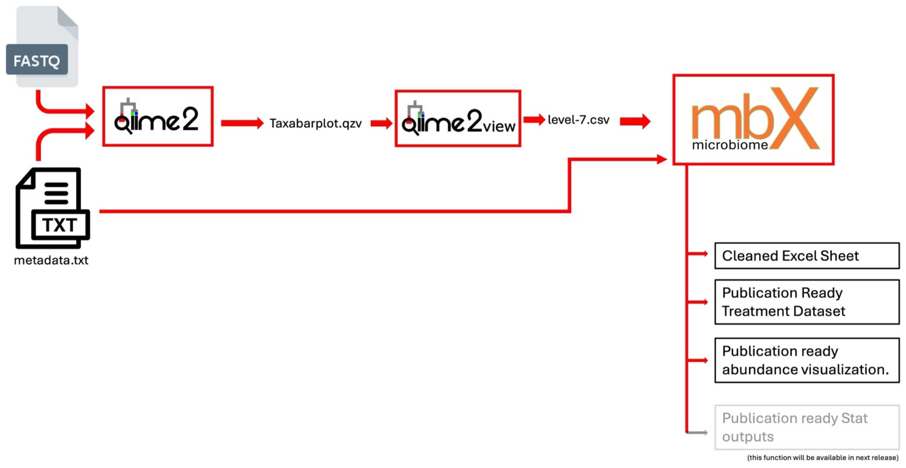
To facilitate easy integration with QIIME 2 outputs, mbX accepts CSV format for the microbiome data as shown in Figure 1. QIIME 2 users can export a taxonomy annotation frequency table by opening the QIIME 2 taxa barplot visualization (.qzv file), selecting the most specific taxonomic level (level 7), and downloading the data as a CSV. This CSV contains the frequency of each taxon in each sample, often including all taxonomic ranks in a single concatenated taxonomy string. mbX’s ezclean function is designed to parse such files. It is important that the CSV include all ranks up to the chosen level (for example, include columns for Domain, Phylum, Class, Order, Family, Genus, and Species). The metadata file can be in CSV, TSV (tab-delimited text), or Excel format; a tab-delimited text (QIIME 2-compatible metadata format) is recommended for consistency. The metadata must have a header row with column names (no spaces in names), and one of those columns should uniquely identify samples (matching the sample IDs in the abundance CSV). In practice, using the exact metadata file from the upstream pipeline (QIIME 2) ensures a smooth merge of raw microbiome data and metadata by mbX.

Figure 1. Schematic overview of mbX’s end-to-end workflow, from QIIME 2-derived abundance tables and metadata through automated cleaning and publication-ready visualizations.

Figure 1. Schematic overview of mbX’s end-to-end workflow, from QIIME 2-derived abundance tables and metadata through automated cleaning and publication-ready visualizations.

Internally, when ezclean is invoked (via a simple R function call such as ezclean (“microbiome_data.csv”, “metadata.txt”, “Family”)), it performs a series of transformations. It first reads the microbiome CSV into R and verifies that sample names correspond to those in the metadata. It then merges the taxonomic data with metadata (appending sample attributes to each sample’s data) and converts raw counts to relative abundances (percentage) to standardize across samples. The function selects the specified taxonomic rank—for instance, if level = “Family”, all taxa are aggregated at the family level. Taxonomic labels are cleaned for consistency. The output is written to an Excel file (.xlsx) named according to the taxonomic level. This Excel file contains a matrix of samples versus taxa with relative abundance values, ready for further analysis or visualization. All outputs are saved with informative, level-specific filenames (e.g., mbX_cleaned_genera.xlsx for cleaned data at genus level), and intermediate files are automatically removed to keep the workflow tidy.

The ezviz function can be run after ezclean to generate plots. In a typical use, the user would call ezviz (“microbiome_data.csv”, “metadata.txt”, “Family”, selected_metadata = “SampleType”, threshold = 0.01) or a similar function signature. Here, selected_metadata indicates the column in the metadata file by which to group samples for visualization (for example, “SampleType” could group samples by gut vs. nasal, or any category of interest). ezviz will take the raw file and user-defined parameters and merge them with metadata grouping information. Once the data are merged, ezviz calculates the mean relative abundance for each taxon within each group (defined by the unique values of the selected metadata factor). By default, it then sorts taxa by overall abundance and retains either the top n taxa (user-defined) or those above a certain relative abundance threshold (user-defined). All remaining low-abundance taxa are summed into an “Other” category. This ensures that the final bar plot remains readable by not overloading it with dozens of tiny slivers representing rare taxa. Users can further limit the taxa shown by specifying top_taxa. For example, ezviz (“microbiome_data.csv”, “metadata.txt”, “Family”, selected_metadata = “SampleType”, top_taxa = 10). This will rank families by their mean relative abundance, display only the ten most abundant, and collapse all remaining taxa into “Other_families”.

The plotting step uses a distinct color palette for taxa and automatically generates figure titles and labels indicating the taxonomic level and grouping (for example, “Relative Abundance of Microbial Families by Sample Type”) (Figure 2 and Figure 3). The output is a high-resolution figure file (PDF format for scalability) as well as an Excel file of the summarized data used in the plot. The figure dimensions and label orientations are dynamically adjusted according to the number of groups and taxa, to optimize readability. Console messages are printed at the major steps while executing ezviz.

2.3. Integration with Upstream Pipelines

A key feature of mbX is its compatibility with popular microbiome workflows. QIIME 2 users can seamlessly use mbX. One simply needs to export the QIIME 2 taxonomic table collapsed at the species (level 7) taxonomic rank or directly download the taxonomy bar plot data as CSV and use that as input to the raw microbiome data to the functions in mbX. The metadata file from the QIIME 2 analysis can be reused for mbX with no modification (ensuring the first column header is an allowed sample ID header). This design makes mbX a convenient extension to QIIME 2, focusing on tasks that QIIME 2’s core plugins do not automate (such as combining taxonomy with metadata in one table and producing custom Excel outputs and plots). The emphasis on simple, standard file formats (CSV for data, TSV/CSV for metadata) means researchers can use mbX as a modular component in their analysis pipeline. All processing in mbX is deterministic given the inputs, so results are fully reproducible; if the same inputs are provided, mbX will generate identical outputs every time.

3. Results

We evaluated mbX on a diverse collection of microbiome datasets to validate its functionality and demonstrate its advantages in data cleaning, visualization, and automation. As shown in

Table 1. Overview of the datasets used for testing.

Study	Number of Samples	Sample Source	Database Used for Taxonomy
1	111	Cattle (lung)	GreenGenes2
2	48	Broiler chicken (ceca)	GreenGenes2
3	34	Layer chicken (ceca)	GreenGenes2
4	1179	Cattle (feces)	GreenGenes2
5	526	Cattle (oral)	GreenGenes2
6	1176	Cattle (rumen)	GreenGenes2
7	60	Bull (semen)	GreenGenes2
8	32	Pig (feces)	GreenGenes2
9	902	Mice (cecal, feces)	GreenGenes2
10	137	Cattle (feces)	GreenGenes2
11	20	Human (feces)	GreenGenes2
12	137	Cattle (feces)	Silva138
13	78	Cattle (rumen)	Silva138
14	20	Soil	Silva138

, a total of 14 independent 16S rRNA gene amplicon datasets classified using GrrenGenes2 [12] and Silva138 [13] were tested, comprising over 4460 samples in total. These datasets spanned a variety of environments and experimental designs, including human gut microbiome profiles, different ruminant microbiomes, chicken microbiome, soil microbiomes, and mouse model microbiome experiments. In each case, we applied the same mbX workflow to the taxonomic output and compared the results to the original analyses or to manual processing approaches.

3.1. Data Cleaning and Standardization

The ezclean function successfully processed all datasets, producing cleaned abundance tables without manual intervention. This included cases with complex taxonomies and varying numbers of taxonomic ranks. We observed that ezclean’s automated formatting resolved common inconsistencies present in raw taxonomy outputs. It also handled samples with zero counts for certain taxa gracefully (filling in zeros in the output matrix as needed, rather than leaving blanks). The output Excel files from ezclean were immediately usable for analysis, with each containing a single table where rows = taxa and columns = samples (plus an additional sheet for any summary if provided, such as total reads per sample). All file names were systematically generated (e.g., mbX_cleaned_phylum.xlsx, mbX_cleaned_genera.xlsx), which allowed us to easily organize results from different levels. We verified the accuracy of ezclean by comparing its output to manually curated versions: the relative abundance values and taxon presence/absence all matched exactly, indicating that no information was lost or altered incorrectly during processing. The automation saved considerable time and avoided user-based errors.

3.2. Visualization and Data Insights

The ezviz function produced stacked bar plots for each dataset, grouping samples by relevant metadata categories. Moreover, the visual outputs were of publication quality, requiring no further editing for clarity and resolution. The thresholding feature proved to be useful for simplifying the results without losing the overall trend. These visual findings were obtained in a very small time through mbX, compared to the manual effort of exporting data and using a separate plotting script. All plots were output as PDFs, which we could directly include in figures for publication without reformatting. Table outputs from ezviz (e.g., mbX_visualization_data_genera.xlsx) also provided the aggregated data underlying each plot, which was helpful for quantitative comparisons. For instance, we could confirm the exact relative abundance values of key taxa and even use that data for additional custom plots (such as heatmaps) outside of mbX. The consistency of mbX’s visualization outputs across all 14 datasets demonstrates the robustness of the tool in handling different microbiome profiles. We did not encounter any cases of the plotting function failing or producing erroneous graphs, even when some groups had very low sample counts (ezviz automatically adjusts and can plot a single sample group as 100% of that sample’s community).

Figure 2. Example of a figure generated by mbX using the ezviz function.

Figure 2. Example of a figure generated by mbX using the ezviz function.

3.3. Reproducibility and Efficiency

Another benefit observed was the reproducibility of the workflow. Because mbX runs through a standardized sequence of steps with fixed inputs, it was straightforward to apply the exact same analysis protocol to every dataset. This is often challenging in microbiome research, where analysts might custom-tune scripts for each study. With mbX, once the function calls were set up for one dataset, we reused them for all others just by changing file names. This uniform approach reduces potential biases that can be introduced when each dataset is handled differently. We also benchmarked the time and computational resources for mbX. All tests were run on an Apple laptop (M1 max chip, 64 GB RAM). The smallest dataset, with 20 samples, was processed by both functions (ezclean and ezviz) in less than 1 s and with less than 1 GB of memory use. In contrast, the largest dataset (containing 1176 samples) was processed at the species level by ezclean in 106.77 s, and by ezviz in 123.996 s. Memory usage was modest (under 1.5 GB) for most of the tasks, and remained below 4.5 GB for the largest dataset with 1176 samples, well within typical workstation limits. This suggests that mbX can scale to reasonably large amplicon studies, and it is feasible to use on personal computers without special hardware additions. By automating file handling (reading/writing) and cleaning, mbX eliminates many opportunities for user error (such as accidentally sorting samples out of order, or mis-labeling a column) that we have encountered in manual analysis. Overall, the results across these diverse datasets underscore that mbX provides a reliable, efficient pipeline for post-processing microbiome data, yielding consistent outputs that agree with expected results and published findings, while significantly reducing the hands-on time required from researchers (

Table 2. Speed and memory used by functions for the three test datasets.

Function	Study ID	Number of Samples	Time for Function Execution at Different Taxonomic Levels (s)							Average Time (s)	Memory Use
			Domain/Kingdom	Phylum	Class	Order	Family	Genus	Species
ezclean	11	20	0.384	0.385	0.392	0.392	0.427	0.449	0.493	0.417	Less than 1 GB
	12	137	3.138	3.269	3.260	3.434	3.674	4.099	4.371	3.606	Less than 1.5 GB
	6	1176	60.452	58.938	61.106	62.566	67.886	86.753	106.77	72.067	Less than 3.6 GB
ezviz	11	20	0.615	0.634	0.644	0.689	0.701	0.780	0.830	0.699	Less than 1 GB
	12	137	3.803	3.914	3.998	4.189	4.447	5.100	5.485	4.419	Less than 1.5 GB
	6	1176	63.215	65.022	65.696	71.457	75.109	97.868	123.996	80.338	Less than 4.5 GB

).

3.4. Example Using Real Data

Our GitHub repository contains a detailed step-by-step tutorial for new mbX users, which can be found here: https://github.com/utsavlamichhane/mbX-R-package/blob/main/easy_tutorial_mbX.pdf. In addition, a real-life example on how to use the package can be found there (https://github.com/utsavlamichhane/mbX-R-package/tree/main/Stats_in_Article). The fully worked example contains 20 samples obtained from the gastrointestinal tract of beef cattle (10 ruminal and 10 fecal samples). In summary, the user can use the following commands to install/load the mbX package in R, and then produce a figure cleaned at the genus level for that dataset:

Install.packages(“mbX”)

library(mbX)

# Clean at Genus level:

ezclean(“rumen_feces_microbiome.csv”,

“rumen_fecal_metadata.txt”,

level = “Genus”)

The above command will convert full taxonomic paths like “d__Bacteria;p__Spirochaetota;c__Spirochaetia;o__Spirochaetales;f__Spirochaetaceae;g__Treponema;s__Treponema_saccharophilum” into genus-only names like “Treponema” in this specific case. Moreover, it will tabulate all the genera and convert them from absolute frequency to relative abundance (percentage for each genus) and save the results as a Microsoft Excel file (.xlsx extension).

Similarly, the following command will load the mbX package and then produce a figure cleaned at the genus-level for the top 10 most abundant genera found in that dataset:

library(mbX)

# Visualize by SampleType (Rumen vs. Feces), showing the top 10 genera:

ezviz(“rumen_feces_microbiome.csv”,

“rumen_fecal_metadata.txt”,

level = “Genus”,

selected_metadata = “SampleType”,

top_taxa = 10)

Figure 3. Visualization generated by the ezviz function: Top 10 genera detected in the ruminal and fecal samples of beef cattle.

Figure 3. Visualization generated by the ezviz function: Top 10 genera detected in the ruminal and fecal samples of beef cattle.

In addition to the visualization, the previous command produces a cleaned genera.xlsx file summarizing the relative frequencies of each genus, which can be used to build visualizations in other software, in case the user is not satisfied with the visualization that was generated by mbX.

4. Discussion

The development of mbX addresses a practical gap in the microbiome bioinformatics toolkit: the need for an automated, end-to-end solution specifically focused on curating and visualizing taxonomic data. While upstream pipelines like QIIME 2 cover read processing and initial analyses comprehensively (including quality control, taxonomic assignment, and diversity metrics), they offer relatively limited functionality for tailored data cleaning and custom visualization of taxonomy tables. For example, QIIME 2 provides standard barplots and basic interactive charts, but exporting data for further modification is often necessary to meet publication requirements, such as trimming taxa names or to integrate with other analyses. In contrast, mbX extends the pipeline by taking those intermediate results and performing the “last mile” of analysis in a consistent, reproducible manner. By automatically merging taxonomy with metadata and generating ready-to-publish figures, mbX simplifies a process that normally would involve multiple tools or custom scripts.

Manual data cleaning in spreadsheets is prone to errors—sample IDs can become inconsistent, grouping variables may be misassigned, and typos in metadata fields often slip through unnoticed. Real 16S datasets also present frequent challenges: missing taxonomic ranks, synonymous names, zero-count artifacts, and ambiguous species-level assignments that can be mistakenly collapsed. In many pipelines, cleaning data at each of the seven taxonomic ranks requires separate scripts or manual reformatting for every level. With mbX, the user can use the same input file (e.g., level-7.csv) and simply change the level parameter in a single ezclean() call—no extra coding needed—to generate cleaned tables at any desired rank. This one-line flexibility ensures consistent, reproducible processing across all taxonomic levels. Importantly, rather than lumping all unassigned species into “Other_species”, ezclean() preserves full resolution by renaming each unassigned entry to reflect its most specific known rank (for example, “Unidentified_species_1_at_Lactobacillus_genus”, “Unidentified_species_2_at_Ruminococcaceae_family”, etc.), ensuring no taxonomic detail is lost. This works not just for species level, but for all taxonomic levels.

Compared to existing R packages for microbiome analysis, mbX is distinguished by its level of automation and ease of use (

Table 3. Comparison of key features offered by mbX, Phyloseq, mothur, and MetaPhlAn.

Feature	Bioinformatics Tool
	mbX	Phyloseq	Mothur 1	MetaPhlAn
Automated data cleaning	Taxonomic standardization, missing-value handling, and level-specific pivot in one call	Requires custom dplyr/phyloseq coding	Manual parsing of “shared” files	No built-in cleaning
Built-in visualization	Publication-ready stacked bar plots	Requires manual ggplot2 scripting	External R/Excel charting	No native plotting
Ease of use	Single-function workflows (2 calls)	Multiple function calls and pipelines	Custom shell/R scripts	Command-line invocation only
Pipeline-agnostic	Accepts any taxa-by-sample CSV	Depends on the phyloseq import functions	Specific to mothur output formats	Specific to MetaPhlAn profiles
Statistical module	In progress (ezstat)	No built-in stats (relies on other R)	None	None

¹ Downstream scripts.

). Phyloseq [1] remains a powerful and flexible framework, supporting many analyses (ordination, diversity, etc.), but it assumes the user will write R code to subset data, create ggplot2 graphics, and so on. mbX, on the other hand, encapsulates common tasks in one or two function calls, making it accessible to those less familiar with R. This design philosophy emphasizes user-friendliness and minimal coding to perform workflows. In our experience, a graduate student or biologist with basic R knowledge can use mbX to generate results without needing to dig into the underlying code, whereas achieving the same with general packages might require writing hundreds of lines of R code. That said, mbX is not intended to replace comprehensive analysis frameworks; rather, it can be used in tandem. For instance, one could use mbX to achieve a cleaned dataset and initial visualizations, then import the cleaned data into other R packages for advanced analysis (ordination, differential abundance testing, etc.) that fall outside mbX’s current scope.

One important advantage of mbX is reproducibility. The consistent output file naming and automated steps ensure that analyses can be repeated exactly. This meets a growing emphasis on reproducible research standards in microbiome science. In practice, an analyst can share the mbX script (with the function calls and parameters used) along with the input data, and collaborators or reviewers can regenerate the key results. This is more transparent than manual spreadsheet manipulation, which is difficult to trace or reproduce. Tools like QIIME 2 also champion reproducibility by using provenance tracking, and mbX complements that by extending reproducibility to the post-processing stage. The use of open-source R means that mbX inherits the benefits of the R ecosystem (cross-platform support, community validation) and can be freely used and audited by anyone. We note that lowering the barrier to entry with such tools could also encourage researchers who might otherwise rely on proprietary software or manual methods to adopt R for microbiome analysis.

Despite its strengths, mbX has some limitations. First, as of its initial release, mbX focuses on taxonomic relative abundances and their visualization; it does not perform upstream processing (one must still use QIIME 2, mothur, or similar to go from raw sequences to a feature table). We envision mbX as one piece of a larger pipeline rather than a one-stop solution for all microbiome analysis needs. Second, the ezstat module is still under development at the time of writing, meaning statistical comparisons (e.g., testing differences in taxa between groups) are not yet automated in mbX. Until ezstat is released, users must conduct statistical tests using other R packages or statistical software. However, because ezclean outputs a nicely formatted data table, it is straightforward to feed that into popular packages or base R functions for statistical analysis. In the future, ezstat aims to simplify this by providing, for example, automatic t-test or ANOVA, or Non-Parametric tests like Kruskal–Wallis for each taxon between groups, which would further streamline the workflow. Another limitation is that mbX’s visualization is currently limited to stacked bar plots. While these are standard for showing community composition, other plot types (area charts over time, heatmaps, etc.) are not directly supported. Users needing those must generate them separately. We plan to expand the visualization options in future updates or allow mbX to output ggplot objects for user customization.

For future enhancements, we are actively working on the ezstat function to integrate statistical analysis. This will likely include methods for differential abundance (comparing taxa frequencies between groups) and summarizing community differences with p-values or confidence intervals. We are considering integrating non-parametric tests and multiple testing correction to provide an automatic “statistics report” alongside the plots. Additionally, we plan to incorporate support for phylogenetic diversity metrics and ordination plots by interfacing mbX with other packages or adding new functions. Another envisioned feature is an interactive mode or Shiny web application for mbX, which would allow users to run the pipeline through a graphical interface and interactively adjust parameters (like the abundance threshold for “Other” category) and see the plots update. This could make mbX even more accessible to researchers with no R experience. Finally, as the field evolves toward multi-omics integration and predicting functional profiles, we see potential in extending mbX’s principles to other data types (for example, 18S rRNA gene for eukaryotic organisms, or functional gene abundance tables). The modular structure of mbX means new functions could be added to handle these with similar ease-of-use.

In comparison to contemporary microbiome analysis tools, mbX stands out by focusing on simplicity and automation in a narrow yet critical segment of the analysis pipeline. It complements rather than competes with full pipelines. By using mbX after QIIME 2 or similar, researchers obtain the best of both worlds: a rigorous upstream analysis and a streamlined downstream processing. This integrated approach can improve overall productivity in microbiome research. We anticipate that mbX will be particularly useful in educational settings and core facilities, where there is a need to process many datasets quickly and generate standardized outputs for collaborators.

In conclusion, mbX contributes to the microbiome bioinformatics landscape by providing a streamlined, reproducible, and user-friendly tool for 16S rRNA gene data post-processing. It empowers researchers to spend less time on data wrangling and plotting and more time on interpreting biological meaning. As microbiome studies continue to grow in scale and complexity, such automated tools are essential for keeping analysis workflows efficient and accessible.