1. Introduction
Latin American elections are typically characterized by a high proportion of blank and null votes (BNVs) [
1]. According to [
2], this type of voting can occur due to socio-demographic, institutional, or political factors. The socio-demographic approach considers economic and social development variables, including literacy rates, education, and healthcare. The institutional aspect encompasses features, such as the compulsory nature of voting (whether mandatory or not), the type of electoral system, the structure of the ballot, and the timing of elections. Finally, in the political sphere, a BNV is seen as a deliberate act of protest driven by voter dissatisfaction with political or economic conditions. However, these classifications do not create mutually exclusive categories, as several theorized causal mechanisms (e.g., protest motives) for null voting correspond to two or more categories and empirical variables. See, for example, [
1,
3,
4,
5].
In electoral systems where voting is compulsory, there is a higher tendency for electoral participation, even when sanctions for abstention are minimal or loosely enforced [
6]. On the other hand, the related literature emphasizes the need to discuss its consequences on voting choices, particularly regarding the quality of electoral decisions [
6]. In this context, an invalid vote is defined as one that is not attributed to any political party or candidate. Such votes lead to ballots that are excluded from the mandate allocation process and primarily consist of BNVs.
Recently, researchers have shown a growing interest in studying this voting behavior, particularly due to its prevalence in various countries. The works of [
1,
7,
8] aimed to identify the factors associated with BNVs in Latin American countries. Ref. [
9] focused their analyses on the occurrence of BNVs in Germany. Ref. [
10] conducted comparisons between Latin America and post-communist Europe, while [
11,
12] centered their analyses on European democracies. Ref. [
13] studied this type of electoral behavior in Western European countries, Australia, New Zealand, and the Americas. Additionally, we can mention [
14,
15] for their contributions focused on the Peruvian and Colombian elections, respectively.
In Brazil, compulsory voting in a political context marked by bribery, nepotism, extortion, and high levels of corruption and scandals increases resentment toward candidates, which is expressed through abstention [
16]. In this way, BNVs can represent protest manifestations perceived as a reaction against specific candidates or policies [
17]. According to the Electoral Glossary of the Superior Electoral Court [
18], a blank vote occurs when a voter refrains from selecting any candidate. Conversely, null votes occur when voters enter numbers that are not valid, i.e., they do not correspond to any candidate. According to Article 211 of the Electoral Code, Law No. 4737/1965 [
19], the candidate “most voted who has obtained an absolute majority of votes, excluding, for the calculation of this, the blank and null votes” is considered elected. Thus, casting a BNV in practice equates to abstention, even if the voter physically participates in the election.
According to [
20], in the 2018 elections, the percentage of null votes was 6.14% in the first round and 7.43% in the second. Blank votes accounted for 2.65% in the first round and 2.14% in the second. Thus, analyzing the dynamics of BNVs contributes to understanding the Brazilian political landscape and society’s stance on the obligation to choose representatives. In this context, the objective of this research is to identify the factors influencing the proportions of BNVs in Brazilian municipalities during the 2018 presidential elections, specifically (i) describing the behavior of the proportion of blank and null votes, (ii) fitting unit regression models to identify the determinants of the proportion of BNVs, and (iii) estimating the impact of the factors identified as determinants of the variable of interest.
Given that the proportion of BNVs is confined within a doubly bounded interval, it is crucial to employ models that account for this constraint. According to [
21], this variable type often exhibits skewness, heteroskedasticity, and, in some cases, heavy tails, which can affect results obtained from models assuming normality. Beta regression [
21] is the classical model for fitting doubly bounded or unit data, as in the case of the proportion of votes. However, simplex regressions [
22,
23], Kumaraswamy (Kw) [
24,
25], unit Weibull (UW) [
26], and reflected unit Burr XII (RUBXII) [
27] have been proposed as alternatives when the beta distribution fails to accommodate the data dynamics.
The aforementioned models employed in this study belong to the Generalized Additive Models for Location, Scale, and Shape (GAMLSS) family [
28]. This flexible framework is particularly suited for analyzing the role of socioeconomic disparities in BNVs during the 2018 Brazilian presidential elections, as it allows us to capture complex parametric relationships that, until now, have not been studied in this electoral context. The importance of this approach lies in the fact that GAMLSS models encompass a wide range of probability distributions and allow for the inclusion of regression structures on multiple parameters of the distribution. The ability to use a variety of distributions, including those with bounded support, makes them particularly suitable for modeling data within the [0, 1] interval, such as BNVs. This flexibility is one of its main advantages, in addition to its ability to handle large data fluctuations (extreme values) and variables with asymmetric behavior, modeling them more adequately than traditional models based on Gaussian distributions. Furthermore, the ease of implementation through well-established R packages has contributed to the growing use of GAMLSS in recent literature [
29,
30,
31,
32]. The results obtained in our analysis within this framework provide valuable insights for advancing the understanding of electoral behavior and democratic participation, especially in contexts of socioeconomic inequality.
The remainder of this paper is structured as follows.
Section 2 presents the definition of the GAMLSS class, which encompasses the unit regression models used in this study.
Section 3 provides a description of the dataset and its construction.
Section 4 presents and discusses the regression models fitted for the proportion of BNVs in the second round of the 2018 Brazilian presidential elections. Finally,
Section 5 offers concluding remarks.
2. Unit Regression Models in the GAMLSS Family
In this section, we present the definition of the GAMLSS class, which encompasses the unit regression models used in the analyses of this work. This class includes semi-parametric regression models, requiring the assumption of a probability distribution for the response variable while also allowing for non-parametric smoothing functions. GAMLSS models were introduced by [
33], with their initial developments presented in [
34,
35]. The objective of this framework was to establish a general class of regression models, encompassing and surpassing some limitations of popular generalized linear models [
36] and generalized additive models [
37].
Let
be a sample of
n independent observations, where each
, follows a probability distribution with a density function denoted by
where
represents the vector of parameters associated with this distribution. In the GAMLSS class, each component of
follows a regression structure, which can also incorporate additive components. Typically,
represents a location parameter and
accounts for precision (or dispersion), while
and
define shape parameters. The structure of the GAMLSS class can be expressed as follows:
where
,
,
, and
. For
,
is a strictly monotonic and twice-differentiable link function that maps
into
;
is the linear predictor;
is a parameter vector associated with the regressor matrix
, which is assumed fixed and known; and
are non-parametric smoothing functions applied to the corresponding explanatory variable
. The matrix
has dimensions
, where
n is the sample size and
represents the number of regressors associated with the
k-th submodel, including a column of ones when an intercept is required. The matrix
has dimensions
, where
represents the number of non-linear regressors associated with the
k-th submodel.
The GAMLSS class is highly flexible [
34], where (i) the response variable is not restricted to the exponential family; (ii) in addition to modeling the location parameter, other distribution parameters can also be included; and (iii) different additive terms can be considered as covariates. Furthermore, the
gamlss package in R enables fitting this model and its subclasses across hundreds of probability distributions. If the required distribution is not available, it is possible to create custom “gamlss.family” objects to extend the package’s functionalities [
34]. This allows for the estimation of unit regression models using these resources.
In the analysis of data constrained to doubly bounded or unit intervals, it is essential to employ suitable distributions. Some notable distributions in this context include beta regression [
21], Kw [
24,
25], simplex [
22,
23], UW [
26,
38], and RUBXII [
27]. These distributions are biparametric, with regression models constructed through reparameterizations involving a location parameter and an additional parameter related to dispersion, precision, or shape. The GAMLSS framework is particularly appropriate in this context, as it allows for modeling not only the response variable’s mean (or other location parameter) but also its variability, facilitating a more comprehensive data analysis. In our study, which deals with proportions that may exhibit heteroskedasticity and skewed behavior, this capability is especially relevant. The regression models presented in the following subsections, which are part of the GAMLSS model formulation, have the following key assumptions: (i) the response variable is continuous and restricted to the interval (0, 1); (ii) the observations are independent; and (iii) the random variable follows a beta, simplex, Kw, UW, or RUBXII distribution.
Further, notice that the general formulation of GAMLSS models allows for incorporating regression structures in a maximum of four distributional parameters, typically referred to as location, scale, and shape. However, the distributions considered in the next subsections are biparametric. As such, the GAMLSS framework, in those cases, includes regression structures only for the two parameters that define each distribution. In this work, we follow the approach adopted in previous studies, such as [
30,
31,
39], who excluded additive components from the model. This approach is based on the fact that restricting the model to linear terms improves the interpretability of the estimated effects since, depending on the chosen link function, we can obtain a straightforward interpretation of the estimated parameters. Furthermore, more parsimonious specifications are generally preferable, which is achieved by excluding nonlinear components as long as the final model is well specified. Moreover, it is worth noting that, to the best of our knowledge, there is a lack of studies considering the additive component for the Kw, UW, and RUBXII regressions. Thus, the models considered take the form
and
where
and
are unknown parameter vectors linked to the linear predictors
and
, respectively. The matrices
and
have dimensions (
) and (
), with
, representing the observed regressors associated with the predictors, which are assumed fixed and known. For these models, the strictly monotonic and twice-differentiable functions
and
(except in the case of beta regression, where
in
gamlss belongs to the unit interval) are used. Furthermore, we employ the logit link function for parameters with a parametric space in the unit interval and the logarithmic link function for parameters with a parametric space over the positive real line. Finally, the systematic components from Equations (
1) and (
2) are combined with the random components of each distribution. The subsequent sections describe these components and the parameterizations used for each distribution.
2.1. Beta Regression
Let
Y be a random variable with a beta distribution, parameterized by the mean
and dispersion parameter
[
40]. Its probability density function (pdf) is given by
where
is the beta function. Under this parameterization, the variance of
Y is given by
Notably, this parameterization is implemented for the beta density in the
gamlss package in
R [
34,
41,
42].
The beta regression model was proposed by [
21], albeit with a parameterization different from that available in
gamlss. Since then, this model has been used to study various practical problems, and some generalizations have been introduced in the literature. For instance, Refs. [
43,
44] proposed beta regression models with parametric link functions. Ref. [
45] developed control charts based on the residuals of beta regression. Additionally, Ref. [
46] suggested specification tests and presented an application to COVID-19 data.
2.2. Simplex Regression
Let
Y be a random variable following a simplex distribution, parameterized by the mean
and dispersion parameter
[
22]. Its pdf is given by
In the context of regression using simplex distribution, one of the earliest contributions was the work of [
47], whose proposal allows for modeling both linear and nonlinear relationships between predictors and the response variable. Ref. [
48] studied the effect of measurement errors on model estimation. Ref. [
49] adopted a Bayesian approach and conducted comparisons with beta regression. Additionally, Ref. [
50] compared beta and simplex regressions to explain homicide rates in the capitals of Brazilian states. The simplex regression model is available in the
gamlss package.
2.3. Kumaraswamy Regression
Let
Y be a random variable following the Kw distribution, parameterized by the median
and the dispersion parameter
[
24]. Its pdf is given by
where
and log denotes the natural logarithm.
The parameterization in Equation (
6) was also employed by [
51] to develop a time-series model based on the Kw distribution. Additionally, Ref. [
52] proposed a generalization of this regression model using the Aranda-Ordaz link function. For recent studies on this distribution, see [
53,
54,
55]. Although Kw regression is not implemented in the
gamlss package, it has been made available by [
56].
2.4. Unit Weibull Regression
Let
Y be a random variable following the UW distribution, indexed by its
-th quantile
and shape parameter
[
26]. Its pdf is given by
where
In this work, we consider
to model the median of
Y, facilitating comparisons with Kw regression. The UW distribution is also part of the extended unit Weibull family [
57] and has been recently introduced in the literature. Consequently, most advancements pertain to studies on the properties of this distribution. See, for example, Refs. [
58,
59,
60]. Although Weibull regression is not available in the
gamlss package, implementations have been provided by [
56].
2.5. Reflected Unit Burr XII Regression
Let
Y be a random variable following the RUBXII distribution, indexed by its
-th quantile
and shape parameter
[
27]. Its pdf is given by
where
We set
to model the median of
Y, enabling comparisons with Kw and UW regressions. The RUBXII distribution is also part of the extended reflected unit Weibull family [
57], and the regression model was recently introduced in the literature by [
27]. Implementations following the
gamlss package approach have been made available by [
56].
3. Data Preparation and Descriptive Analysis
In this section, we describe the database and its construction. This study is based on a cross-sectional dataset, where the variable of interest is the proportion of blank and null votes observed in each Brazilian municipality during the 2018 presidential elections. The data were obtained from the database of the Institute of Applied Economic Research [
61], which compiles economic, financial, demographic, geographic, and social data for Brazilian municipalities and states. Additionally, open databases provided by the Brazilian Institute of Geography and Statistics [
62] and the Atlas of Human Development in Brazil [
63] were consulted.
Municipalities with missing data for any of the variables included in the analysis, as well as those created after 2010, were excluded. These exclusions correspond to 16 municipalities: 1 in the North region (Mojuí), 6 in the Northeast (Trancoso, Olivença, Cococi, Messejana, Vertentes do Lajeado, and Nazária), 2 in the Central–West (Figueirão and Paraíso das Águas), 3 in the Southeast (Ponte de Itabapoana, São João Marcos, and Santo Amaro), and 4 in the South (Porto de Cima, Pinto Bandeira, Pescaria Brava, and Balneário Rincão). After these exclusions, the final dataset comprises 5562 observations.
Table 1 presents the variables considered in the analysis, along with their respective sources and descriptions. All the variables are quantitative, except for
Region and
Capital, which are categorical. The variable
Region indicates the geographic region to which each municipality belongs, while
Capital identifies whether the municipality is a state capital.
For the regression models, the Capital variable is transformed into a dummy variable that takes the value one if the municipality is a state capital and zero otherwise. Region is treated as a polytomous variable, with the Central–West region defined as the reference category. Dummy variables are created for the other regions, assuming the value one if the municipality belongs to the respective region and zero otherwise.
The variables PBNVF and PBNVS denote the proportion of BNVs in the first and second rounds of the 2018 elections, respectively. These proportions are computed as the ratio of the total number of BNVs to the overall number of votes cast.
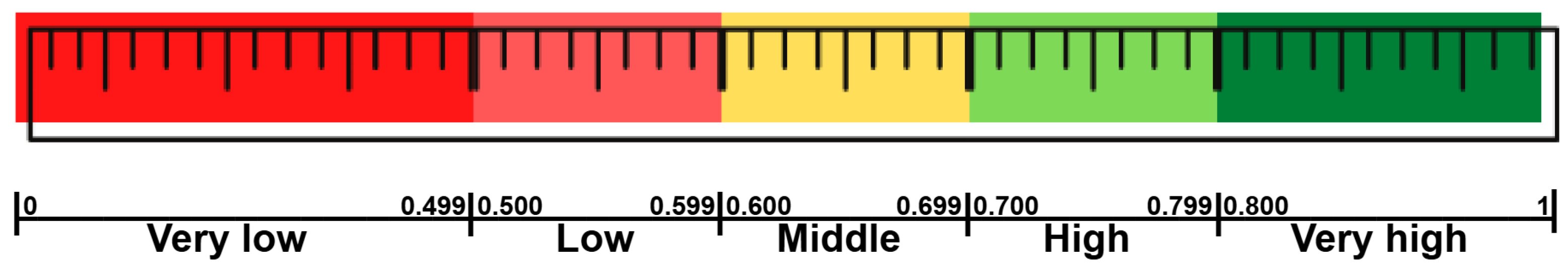
One of the key explanatory variables is the municipal human development index (MHDI), a numerical indicator ranging from 0 to 1. As illustrated in
Figure 1, lower values indicate worse conditions, while higher values reflect better socioeconomic conditions. In this study, we use the disaggregated MHDI, which consists of three dimensions: income, health, and education. This allows for the estimation of their individual effects. The variable
MHDI_I measures the average ability of a municipality’s population to acquire goods and services.
MHDI_H incorporates information on life expectancy and mortality, while
MHDI_E quantifies the educational level of both the adult and young population.
Lastly, the demographic density (DD) of the municipalities is included as an explanatory variable. This indicator is defined as the ratio of the total number of inhabitants to the land area of the municipality.
Table 2 presents the descriptive statistics of the response variable and the quantitative covariates.
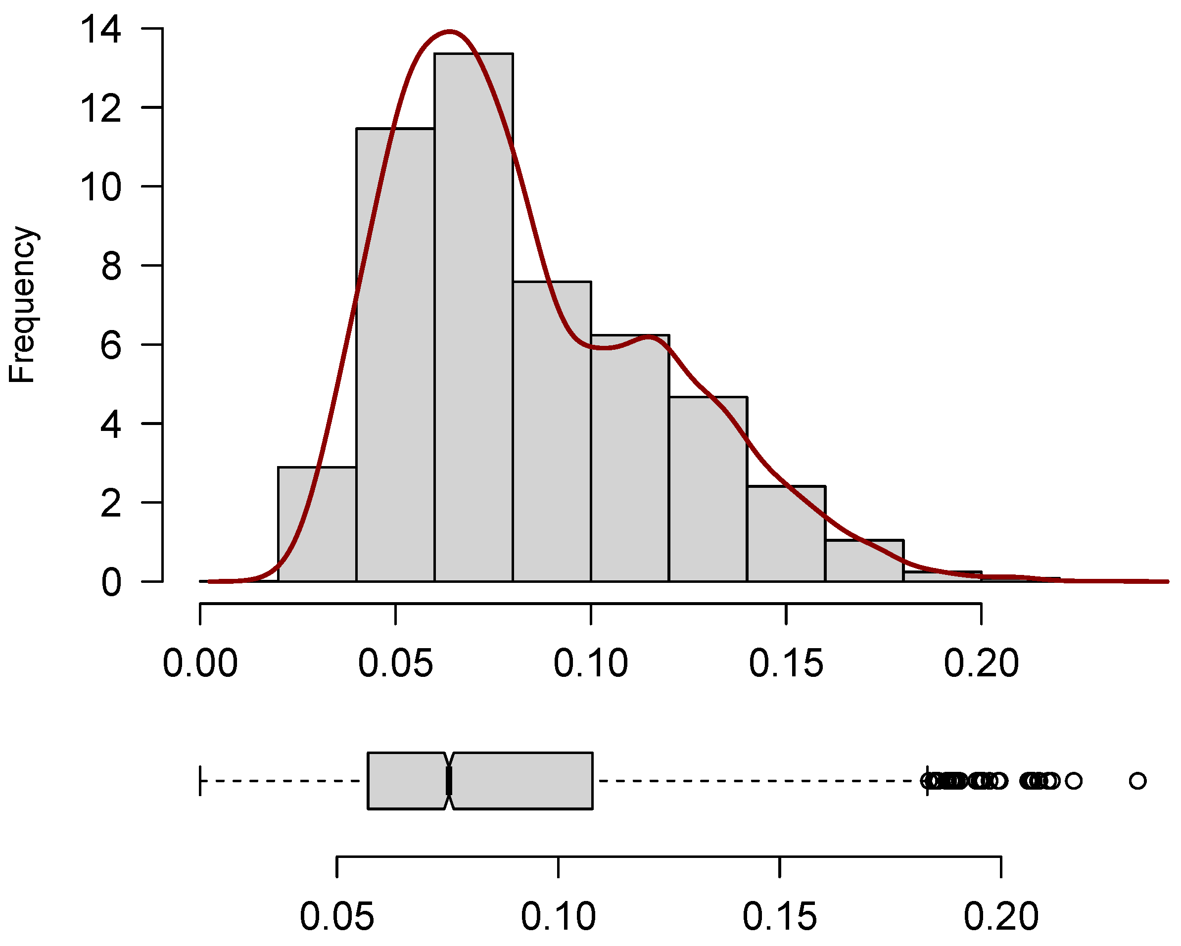
The variable PBNVS presents a mean of 0.08 and a median of 0.08, indicating that the central tendency of the distribution is concentrated around 8%. The minimum and maximum observed values are 0.02 and 0.23, respectively, resulting in a range of 0.21. The distribution exhibits positive skewness (0.77), evidencing asymmetry to the right, with a concentration of municipalities around lower values and a tail extending toward higher proportions. The kurtosis coefficient (0.02) suggests a platykurtic distribution, with thinner tails and a flatter peak compared to the normal distribution. Furthermore, the coefficient of variation (41.33%) denotes a high degree of relative dispersion, reinforcing the heterogeneity of the PBNVS across municipalities. These empirical characteristics justify the adoption of flexible distributional assumptions at the modeling stage.
Figure 2 presents the boxplot and histogram of the variable
PBNVS. The correlations were computed using Spearman’s method, as shown in
Table 3. The results indicate that the response variable exhibits a positive correlation with most covariates. The strongest correlation with
PBNVS is observed for
PBNVF, followed by
MHDI_H. This suggests that these covariates play a relevant role in this study, as they are associated with variations in the response variable.
Figure 2 further substantiates the descriptive findings. The histogram, constructed using relative frequencies and overlaid with a density estimate, reveals a pronounced concentration of observations between 0.05 and 0.10, with a visible mode around the central value. The positively skewed shape of the density function confirms the asymmetry previously noted, suggesting that most municipalities present relatively low levels of blank and null votes, while a smaller subset exhibits notably higher proportions.
The smooth decline of the density curve toward the right tail reinforces the presence of rare but influential extreme values. The boxplot displays a median consistent with the reported central tendency and highlights the presence of upper outliers. These outliers, in conjunction with the interquartile range, reflect the substantial heterogeneity across observations and the long right tail of the distribution. Together, the histogram and boxplot emphasize the asymmetric, dispersed, and bounded nature of the data, reinforcing the choice of continuous distributions defined on the (0,1) interval and capable of capturing such features in the modeling stage.
Table 3 presents the Spearman correlation coefficients between the proportion of blank and null votes in both rounds (
PBNVF and
PBNVS) and the selected covariates. A moderate and significant correlation is observed between the two voting rounds (
;
p < 0.005), indicating partially consistent behavior across elections.
PBNVS exhibits significant positive correlations with all the dimensions of the municipal human development index (MHDI), especially with health (MHDI_H, ) and income (MHDI_I, ), suggesting that higher development levels are associated with increased blank and null voting in the second round. In contrast, PBNVF shows negligible and mostly non-significant associations with the MHDI indicators.
Demographic density (DD) is positively and significantly correlated with both voting variables and all the MHDI dimensions, indicating that more densely populated municipalities tend to show higher development levels and greater proportions of blank and null votes.
Table 4 presents the frequency distribution of the
Region variable. Approximately 50% of the municipalities in the sample belong to the
S and Southeast regions, which are also the most developed in the country. Conversely, the
N and
NE regions, which exhibit lower socioeconomic indicators, account for about 40% of the observations. This regional structure mirrors the official territorial organization and the administrative concentration of municipalities in Brazil, particularly in the Northeast. Given these disproportions, regional stratification may play a relevant role in the variability in the response variable and covariates, potentially introducing spatial heterogeneity to be accounted for in the modeling process.
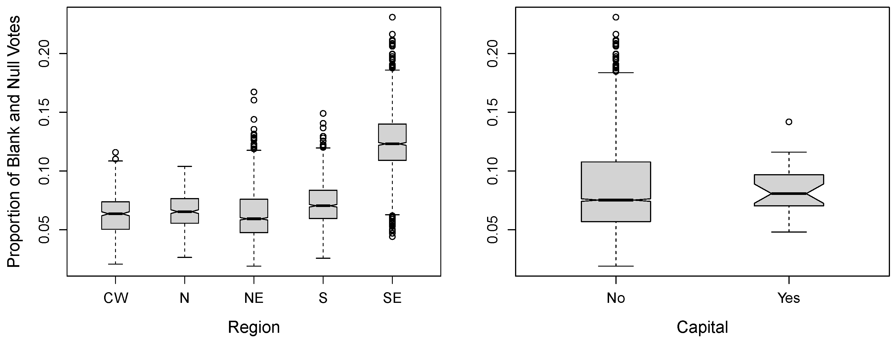
Figure 3 displays boxplots of the
PBNVS according to the
dummy variable
Capital and the
Region variable. Regarding the relationship between
PBNVS and
Region, the
S region stands out from the others. It exhibits the highest central tendency and greatest variability, with a wide interquartile range and the highest maximum value. In contrast, the
NE region shows the lowest median, despite the presence of some upper outliers. The remaining regions display intermediate values with relatively compact distributions. These differences reinforce the presence of regional heterogeneity and support the inclusion of the geographic region as a relevant covariate in the modeling process. In the comparison between
PBNVS and
Capital, a higher incidence of outliers is observed in non-capital municipalities.
4. Fitting the Unit Regressions
This section presents and discusses the regression models fitted considering
PBNVS as the dependent variable. Parameter estimation for all the models was performed using the maximum likelihood method with the Rigby and Stasinopoulos (RS) algorithm [
42]. Model selection was based on the Akaike information criterion (AIC) and the Bayesian information criterion (BIC).
As suggested by [
42], the complete model including all the covariates for both the location (
) and dispersion (
) submodels was initially fitted for all candidate classes, i.e., beta, simplex, Kw, UW, and RUBXII random components.
The specification presenting the most favorable information criteria was then subjected to a stepwise selection procedure for further refinement, ensuring parsimony without compromising model performance.
The explanatory variables considered included socioeconomic indicators, electoral information, and regional effects. The categorical variable Region was represented by dummy variables, with the CW region used as the reference category. The binary variable Capital, indicating whether the municipality is a state capital, was initially included in all the models. However, in the models employing the Kw, UW, and RUBXII distributions, the inclusion of Capital in the dispersion submodel led to convergence issues during the parameter estimation. To address this, the variable was excluded from the -submodel in these cases, ensuring stable and reliable model fitting.
Table 5 presents the estimated coefficients, corresponding standard errors, and associated
p-values for the complete models. All the models incorporate submodels for both the location (
) and dispersion (
) parameters.
We observe that, for the location submodel, most distributional classes yielded coefficients with similar magnitudes and directions. The only exception is the variable MHDI_I, which appears with a negative coefficient for the Kw and RUBXII models and a positive coefficient for the other classes. In fact, there is a noticeable similarity in the estimated coefficients of all the covariates across these models. The beta and simplex distributions also show similarity in their estimated values. This result is expected, given that the beta and simplex models are parameterized in terms of the mean, whereas the others are parameterized in terms of the median.
There is a strong negative association between MHDI_E and PBNVS. This suggests that improvements in local educational attainment are consistently associated with lower levels of electoral disengagement. On the other hand, the health-related component (MHDI_H) exhibits a generally positive effect, indicating that municipalities with better public health infrastructure may display higher rates of blank and null voting. This relationship may reflect underlying behavioral or institutional phenomena, such as protest voting or political disaffection in areas with relatively higher access to public services.
In contrast, the income dimension (MHDI_I) shows a more nuanced effect. While some models suggest a negative association with the proportion of blank and null votes, the magnitude and significance of the estimates vary depending on the distributional assumptions. This variability may reflect the complex interplay between economic conditions and political engagement, where income alone may not fully capture socio-political motivations behind non-nominal voting behavior.
The regional dummy variables also play a significant role in capturing structural heterogeneity across the Brazilian territory. Even after accounting for human development indicators, the Southeast region exhibits higher average levels of blank and null votes, which points to regional cultural or political dynamics not fully captured by conventional socioeconomic variables. The inclusion of regional effects proves crucial for mitigating omitted variable bias and improving model calibration.
From a distributional standpoint, all the models exhibit similar signs and relative magnitudes for the covariates, but subtle differences in standard errors and p-values reveal the sensitivity of inferential conclusions to distributional misspecification. While the beta and simplex models are well suited for symmetric or light-tailed data, they may struggle with asymmetric patterns, particularly near the boundaries. In contrast, the Kumaraswamy, unit Weibull, and especially the RUBXII distributions demonstrate greater adaptability to skewness and tail behavior. The RUBXII distribution, derived from a reparametrized Burr XII, proves particularly robust in handling extreme proportion values, though it introduces additional computational complexity and parameter interpretation challenges.
Model performance was further assessed using information criteria and goodness-of-fit metrics, with the AIC, BIC, and pseudo-
(RSQ) values summarized in
Table 6. In addition, predictive accuracy was evaluated through standard forecasting metrics, namely, the mean absolute percentage error (MAPE), mean absolute error (MAE), and root mean squared error (RMSE), providing complementary insights into the models’ predictive capabilities. These metrics serve complementary roles: the AIC and BIC balance goodness of fit and model parsimony, while the RSQ and residual-based error assess predictive accuracy. The results indicate that the beta regression model achieved the lowest AIC and BIC values. Regarding the RSQ, the RUBXII, Kw, and beta models showed the highest values, respectively. In terms of predictive accuracy, all the candidate classes presented similar MAE and RMSE values, differing in the fourth decimal, with the UW model obtaining the lowest MAPE (approximately 17%). Given that the MAPE, MAE, and RMSE values are relatively low, it can be concluded that all the models provided satisfactory predictive accuracy.
The one that performed best across the majority of the evaluation metrics was selected. Based on this criterion, the beta regression model was identified as the most appropriate. Once the beta distribution was selected as the random component in the GAMLSS regression, we refined its specification using a stepwise model selection procedure. To this aim, we used the AIC as the selection criteria at the
stepGAIC function in the
gamlss package and then checked the significance of the regressors to include only those that are significant at the 5% level. We refer to the final model selected through this procedure as Model A. To formally assess the effect of the regressors on the variance of the
PBNVS, we considered the relationship between the
parameter and the variance of the beta distribution, presented in Equation (
4), interpreting
as an indicator of data heterogeneity. In addition, we fitted a version of the model assuming constant dispersion, which we refer to as Model B.
Table 7 presents the estimates, standard errors, and
p-values of the final model and its constant-dispersion competitor.
The comparison between Models A and B reveals that, while the general directional relationships between the dependent variable and the regressors are preserved across both models, the magnitude of the coefficients varies. These variations highlight the impact of assuming constant dispersion in Model B, which may lead to biased estimates and underscore the necessity of appropriately modeling dispersion in regression analyses.
Since both models are nested, we conducted a Likelihood Ratio Test (LRT) to evaluate whether incorporating covariates into the dispersion submodel enhances the model’s fit. The null hypothesis of the LRT is that the simpler model is preferred. The LRT yielded a test statistic of 279.12 with a p-value < 0.001. Therefore, we reject the null hypothesis at any conventional significance level, concluding that including additional predictors in the dispersion submodel significantly improved the model fit compared to the simpler nested alternative.
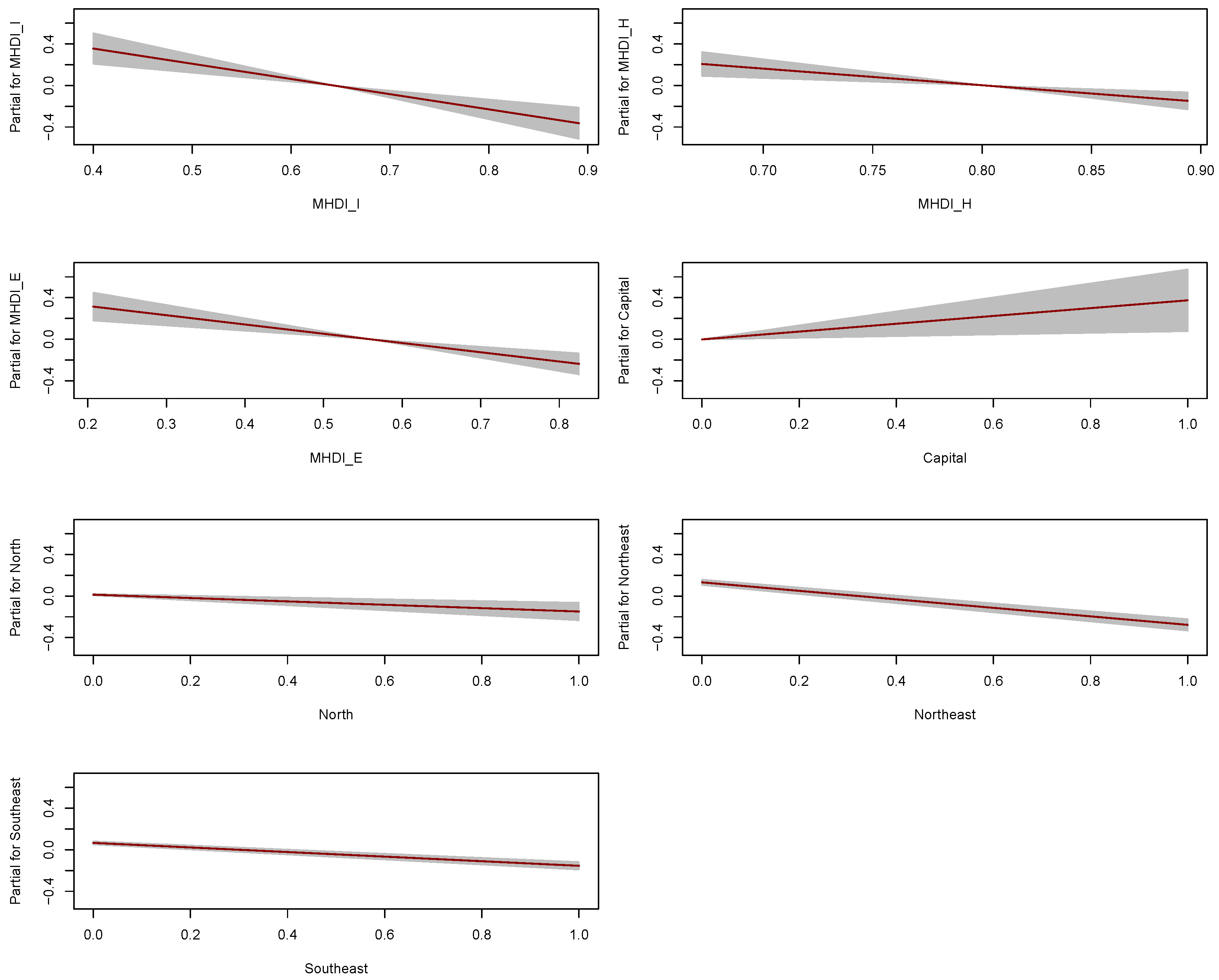
These findings are further visualized in
Figure 4, which displays the partial effect plots for each predictor in the dispersion submodel. The shaded bands represent 95% confidence intervals, confirming the strength and direction of these effects. Notably, all the effects are nearly linear, indicating that the systematic component and the link function specified for
is appropriate and the model fit is stable.
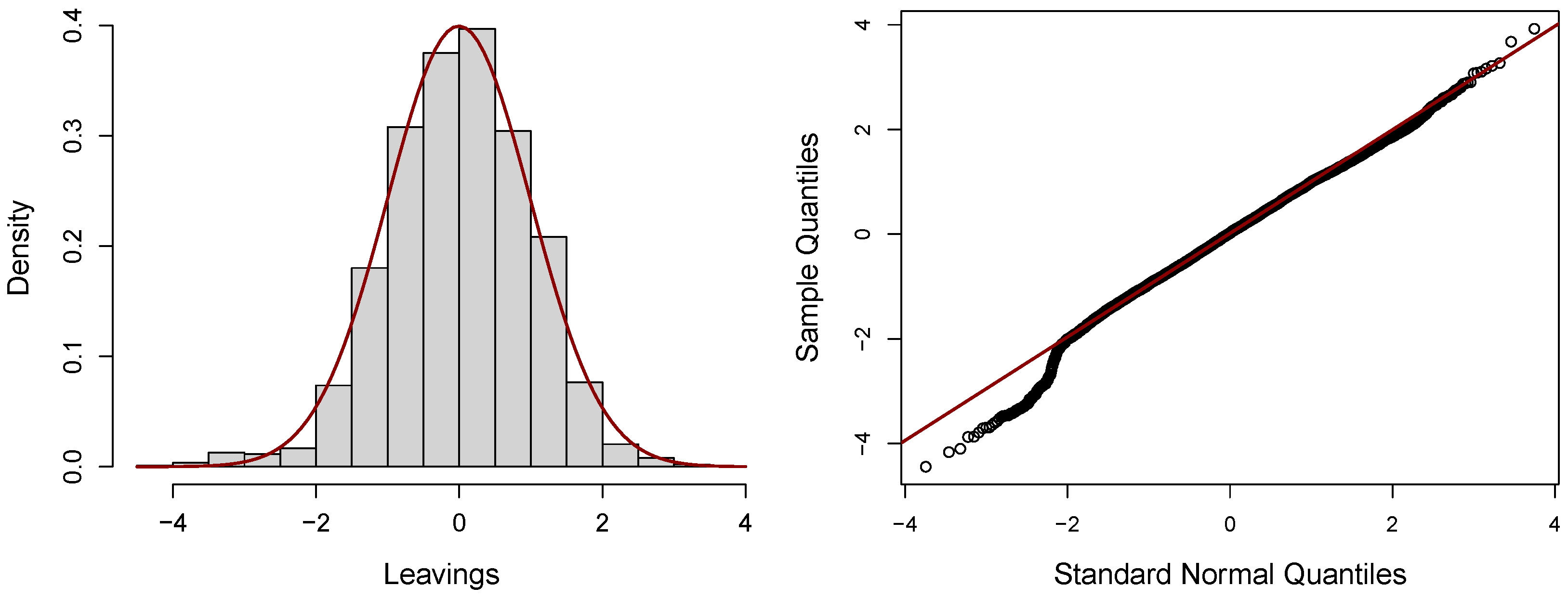
Based on these results, the beta regression with variable dispersion (Model A) is selected as the final model, and the next step is to perform residual analysis as a diagnostic technique to assess the adequacy of the model fit. According to [
64], if the model is correctly specified, the distribution of quantile residuals should approximate a standard normal distribution.
Figure 5 displays the histogram of the residuals from the beta regression, which suggests a tendency toward normality. Additionally, the quantile–quantile plot (QQ-plot) of the quantile residuals is provided. The results support the adequacy of the beta regression model, as the histogram closely resembles a normal distribution, and most of the points in the QQ-plot align well with the 45-degree reference line. This is further supported by the Filliben correlation coefficient of
, close to one, as well as the residual summary statistics, the mean near zero (
), variance close to one (
), slight negative skewness (
), and kurtosis (
), all of which reinforce the appropriateness of the fitted model.
Therefore, the final estimated location submodel takes the following form:
The dispersion submodel controls for the variability in the response across observations. The final dispersion submodel, reflecting these sources of heterogeneity, takes the following form:
From Equations (
7) and (
8), several insights regarding the
PBNVS, assuming fixed levels of the other variables, can be drawn:
The
MHDI_H also shows a positive effect, indicating that municipalities with better health outcomes tend to have more blank and null votes. This result suggests that more significant health development could be linked to lower political participation, possibly due to social problems or disillusionment with the electoral system in these areas. Also, higher socioeconomic development and urbanization contribute to the wider circulation and more democratic access to the political information necessary for voting in national elections [
1].
The variable
MHDI_E shows a negative effect on the
PBNVS, suggesting that municipalities with better educational outcomes tend to have a lower
PBNVS. This indicates that better education is associated with greater political awareness and participation, which translates into fewer protest votes or disengagement from the electoral process. Education and literacy play a crucial role in shaping the political competence of individual voters [
1].
The effects on the Region variable show that geographic location significantly influences the PBNVS. Municipalities in the Southeast region, for example, have the highest PBNVS, indicating a notable regional tendency toward protest or disaffection voting in this area. Other regions, such as the North and South, also show positive effects, albeit to a lesser extent. These results suggest that regional factors, such as the local political climate, and other regional conditions, such as cultural influences, significantly influence voting behavior.
The dispersion model shows that the IDMH_I significantly reduces variability in the PBNVS, meaning wealthier municipalities tend to have more stable voting patterns. Regional effects also play a role, with the SE, NE, and N regions showing negative coefficients, indicating lower variability in these regions.
5. Final Considerations
This study provides a comprehensive analysis of the socioeconomic and regional determinants of blank and null votes in the second round of the 2018 Brazilian presidential elections. By employing flexible GAMLSS models tailored for proportions, we rigorously evaluated five distinct unit regression distributions—beta, simplex, Kumaraswamy, unit Weibull, and reflected unit Burr XII—each capturing different distributional characteristics of the response variable.
Among the tested models, the beta regression exhibited the lowest AIC and BIC values. In terms of accuracy measures (MAPE, MAE, and RMSE), the models yielded similar results. Given these results, the beta regression was chosen as the most appropriate model for analyzing the proportion of BNVs.
Regarding the explanatory variables, MHDI_I, MHDI_H, and MHDI_E, along with the regional classification of municipalities, were the most influential factors affecting the mean proportion of blank and null votes. Specifically, municipalities with a higher MHDI_I and MHDI_H exhibited higher proportions of BNVs, while MHDI_E had a negative effect. Regionally, municipalities in the Southeast had higher average proportions of blank and null votes. Additionally, MHDI_I was found to negatively impact the variability in BNVs, while the Northeast, North, and Southeast regions exhibited distinct effects on the dispersion of the vote proportion.
This study provides insights into the Brazilian political landscape by identifying key factors influencing voters’ decisions to invalidate their votes. The model incorporates socioeconomic, demographic, and political variables, highlighting how regional differences, income levels, education, and political polarization shaped voter behavior during the 2018 elections. The findings may also aid political actors in shaping campaign strategies, as voters who annul their votes represent a potential audience that could be engaged in future elections.
A limitation of the model is its inability to separate the various motivations underlying blank and null votes, such as protest votes, disillusionment, or mere disinterest in the electoral process. The analysis considers BNVs in an aggregated manner, without distinguishing the specific reasons that lead voters to invalidate their votes.


 ,
, 
