Abstract
Developing accurate predictive models in statistical analysis presents significant challenges, especially in domains with limited routine assessments. This study aims to advance the theoretical underpinnings of longitudinal logistic and zero-inflated Poisson (ZIP) models in the context of small area estimation (SAE). Utilizing data from the Canadian Healthy Infant Longitudinal Development (CHILD) study as a case study, we explore the use of individual- and area-level random effects to enhance model precision and reliability. The study evaluates various covariates’ impact (such as mother’s asthma, mother wheezed, mother smoked) on model performance to predict child’s wheezing, emphasizing the role of location within Manitoba. Our main findings contribute to the literature by providing insights into the development and refinement of small area models, emphasizing the significance of advancing theoretical frameworks in statistical modeling.
1. Introduction
Predictive modeling in statistics often involves estimating parameters within complex data structures. This paper focuses on the theoretical development of longitudinal logistic and zero-inflated Poisson (ZIP) models, addressing challenges posed by small sample sizes and sparse data. The context of asthma prevalence in Manitoba serves as a case study to illustrate these models’ application. However, the primary objective is to advance the theoretical framework and methodologies underlying these models, beyond asthma-specific applications.
Asthma is a chronic disease characterized by airway inflammation, leading to variable expiratory airflow limitation and symptoms such as shortness of breath, chest tightness, coughing, and wheezing [1]. In Canada, asthma prevalence is highest among individuals aged 1–34 years [2], with incidence rates gradually increasing each year, particularly among younger demographics [3,4]. Manitoba, a sparsely populated province with the majority of its population concentrated in Winnipeg, presents unique challenges in studying asthma due to small sample sizes in many areas.
This study aims to develop robust statistical models for small area estimation (SAE) to assess childhood wheezing—a symptom of asthma—and its associated risk factors, leveraging longitudinal data from the Canadian Healthy Infant Longitudinal Development (CHILD) study. By focusing on methodological and statistical techniques, this study seeks to enhance the precision and accuracy of estimating wheezing severity across different regions of Manitoba.
To address the issue of small sample sizes, we employed small area models to analyze wheezing rates across different regions. A “small area” is defined as any domain for which direct estimates of adequate precision cannot be produced [5]. Small area models leverage auxiliary variables and random area effects to improve predictions of wheezing rates and severity in geographical areas [5]. Our goal is to refine the theoretical framework and methodologies of these models, advancing the field of small area estimation and providing more accurate and reliable estimates for public health research.
Longitudinal logistic models are designed to handle binary or ordinal response variables, particularly when data are collected over multiple time points. These models account for within-subject correlations and allow for the inclusion of random effects. In this study, we utilized hierarchical Bayesian logistic models to estimate the probability of wheezing severity at different follow-ups, incorporating individual-, area-, and interaction-level random effects.
ZIP models are suitable for count data with an excess number of zeroes, which is common in longitudinal health studies. These models assume that the population consists of two groups: those who never experience the event (always zero) and those who may experience the event (Poisson-distributed counts). The ZIP models in this study incorporate area and follow-up level effects to address overdispersion and excess zeros in wheezing episode counts.
The Canadian Healthy Infant Longitudinal Development (CHILD) study provided a unique opportunity to explore these theoretical advancements. The CHILD study includes detailed longitudinal data on childhood wheezing and associated risk factors, collected from a cohort of children born between 2008 and 2012 and followed up until 2.5 years of age. The data were first accessed for this study on 6 June 2020. The time points for this study were prenatal, 3, 6, 12, 18 months and 2 and 2.5 years. The Manitoba sub-cohort was used for this study and members were recruited within a radius of Winnipeg and Morden-Winkler; families who moved out of this region were still followed. For this particular study, participants were assumed to have the same location throughout the study. This was done using postal codes from the 2-year follow-up, since this follow- up contained the most unique postal codes. Furthermore, individuals with incomplete follow-ups for postal codes or missing postal codes were removed, which resulted in a sub-cohort of 690 families. The responses from the home environment questionnaire indicated that between 80 and 100 participants moved between each follow-up in Manitoba. The primary outcome of the CHILD study was expert physician diagnosed asthma, but wheezing was one of the secondary outcomes. However, it can be challenging to make a diagnosis of asthma in children aged five years since it is not possible to have routine airflow limitation measurement within younger age groups [1]. Wheezing symptoms, however, can still be present in children under five years old. Thus, the difficulty of diagnosing asthma in younger children means that wheezing can be used as an indicator of “possible” asthma diagnosis in the future [6].
For the purpose of this study, Manitoba was divided into small geographical regions (areas) and thus more information was provided regarding which regions had higher rates of wheezing and which factors contributed. The province has five regional health authorities (RHAs) created from the initial eleven RHAs in 2012. These five RHAs are further divided into 96 regional health authority districts (RHADs); these RHADs were intended to be used as small areas for this study. However, for this study, only 60 of the 96 RHADs were recruited by the CHILD cohort. Thus, the 60 recruited RHADs were used as small areas in this study and the RHADs which were not recruited were greyed out in the figures throughout this study. The Manitoba sub-cohort, comprising 690 families, was used to analyze wheezing severity and its predictors.
By employing hierarchical Bayesian logistic models and ZIP models, we aimed to identify significant predictors of wheezing severity and rates, such as maternal asthma, smoking, and environmental factors. The integration of individual- and area-level covariates allowed us to capture the variability within small areas and enhance the precision of our estimates.
2. Small Area Models
2.1. Linear Mixed Model
Basic types of small area models are area-level and unit-level models. Area-level models are also called aggregate models, which relate small area means to area-specific auxiliary covariates [5,7,8]. Unit-level models relate the unit values within a small area to unit-specific auxiliary variables. Unit-level auxiliary variables provide individual-level information [9]. Assuming the response of the model is , the parameter of interest is a function of the small area means for area k such that . In this case, is the link function that connects the response with the covariates and random components of the model. In the case of the linear model, the link function is the identity, for the case of the logistic model, the link function is logit, and for the Poisson model, the link function is log. It is crucial to understand that the end goal of small area analysis is to estimate the small area parameter . Assume the indirect estimator of is
where K is the number of small areas and the error terms ( are independently and normally distributed with mean 0 and variance . Note that it is assumed that is known to avoid identifiability issues. Further, if area-level auxiliary data are available then a linear model can be formed as
where ’s are the known positive constants; these are to set optional different random effects for each small area. The term represents the area-specific random effects with the assumption that all ’s are independent and identically distributed (iid) with mean 0 and variance , as denoted by . Note that ’s are assumed to be normally distributed but are not limited to this distribution. Lastly, is a vector of regression coefficients. Combining (1) with (2) results in
which is the final form of the basic area-level model and is also referred to as the Fay–Herriot (FH) model [10]. Now, if there are unit-specific auxiliary data available within each small area, then the basic unit-level linear model can be used to model small areas. Assuming that i is any element, say an individual within any small area k, and represents the sample size in each area, then the model is
In Equation (4), are the auxiliary data and are the corresponding regression coefficients. Like the FH model, represents the area-level random effects while the sampling error is with known constants but unknown variance . It should be kept in mind that the parameters of interest like the FH model are the small area means, . Note that one can also incorporate area-level and unit-level covariates into the unit-level model (4) as is the case for the CHILD cohort.
In general, to estimate small area means, the best predictor (BP) is used. The BP of a parameter of interest, such as the small area mean is the conditional expectation of the parameter given the data and the model parameters. Thus, the BP assumes that the model parameters are known. The BP does not have a closed form for most non-linear models. Thus, numerical methods were needed to estimate such models. In particular, Bayesian methods were used for this study; hence, diffuse priors were implemented on the model parameters and .
2.2. Logistic Mixed Model
Suppose now that is binary, and we are interested in the small area proportions , , then the hierarchical Bayesian (HB) area-level logistic model [7,8] is
and priors,
Note the diffuse prior chosen for the inverse of variance parameters is a gamma distribution with shape and location parameters 0.001 (). If unit-specific auxiliary data are available within each small area, and we are interested in the small area proportions , , where is the number of individuals in area k, then the unit-level logistic model is
and priors,
2.3. Poisson Mixed Model
Now, we consider the count data in the response by assuming that are area-level counts and are distributed Poisson variables [7,8]. The parameter of interest in this model would be , the true average rate of wheezing in the area. Thus, the model becomes
where and The same priors as in Section 2.2 were used for and .
2.4. Inference
A Monte Carlo Markov Chain (MCMC) was used to estimate the parameters of interest for the above models (5), (6), and (7). We used the R package Rjags to implement the MCMC. All models in thus study were run on Rjags; the initial models had 200,000 iterations with a thinning degree of 18. Diagnostic tools such as the Gelman–Rubin test were used to determine if the model converged to the target posterior distribution. The Gelman–Rubin diagnostic evaluates MCMC convergence by analyzing the differences between multiple Markov chains—a small within-chain variance indicates convergence [11]. Thus, multiple chains were sampled from each, with burn-in to ensure accurate results. If the initial model did not converge according to the Gelman diagnostics for all covariates, then the model was updated each time with 10,000 iterations. The model was updated until convergence was reached. Additionally, the 95% credible intervals for the posterior distributions were calculated using the equal-tail interval method, which is the default method in Rjags. Particular attention was made to the choice of priors and structure of the random effects. The Deviance Information Criterion (DIC) was used for model comparison and to determine model adequacy. DIC is often viewed as a trade-off between model adequacy and complexity [12]. DIC statistics were used throughout the model building stages of this study.
3. Proposed Statistics Models
For the CHILD study, our interest was to determine which factors affected the rate of wheezing and severity over time (follow-ups) along with geographical information. Wheezing severity was either a binary or an ordinal variable; thus, longitudinal logistic area models were required [13,14,15]. Furthermore, a model to analyze the number of wheezing episodes was needed for each follow-up. Thus, extensions of the logit (6) and Poisson (7) models were needed for this study. In general, the models have different link functions dependent on the type of response variable. In the context of the CHILD study, the response was dependent on participant i, follow-up j, and area k. Assuming, without loss of generality, the model has three random effects which can depend on any combination of i, j and k and with response variable and corresponding , then, letting , we obtain,
In Equation (8), was the random effect of the individual and follow-up. In this model, we assume the disturbance is an AR(1) (autoregressive-one) effect. is the interaction random effect of all three levels interacting with one another and is simply the random effect of each small area.
From model (8), is the link function that connects with the covariates and random components of the model. The link functions of interest for this study were the logit and log, as shown below in Equations (9) and (10), for the logistic and Poisson models, respectively. The logit link function is used when the response variable is assumed to follow a binomial, multinomial or ordinal distribution (e.g., a child wheezed or not in our CHILD study). The log link function is primarily used when the response is assumed to follow a Poisson distribution (e.g., wheezing episodes in our CHILD study). So, accordingly, we have
The three types of models of interest for this study were as follows.
3.1. Ordinal Logistic Model
A logistic model with the assumption that the response, , is ordinal was used to quantify how much of an impact location and time had on wheezing severity. Here, represented the childhood wheezing severity of child i in a particular area k at follow-up j.
Now, the ordinal logistic model is described. In our CHILD study, have three levels ; thus, there are two categories (with another level as a reference category). We then obtain
where i represents the individual, j is follow-up, and k is the small area, and
Thus, the two logit equations with are
Note, in this case, the vector of covariates does not include the intercept term since this is represented by and . In general, was a level specific intercept with the restriction that such that .
3.2. Binary Logistic Model
Due to the lack of viable data, the severity of wheezing response variable was transformed to two levels. This was accomplished by merging responses 2 and 3 into one level, as the numbers in these two levels were small compared to level 1. The resulting model is described as follows:
Then, is the probability that the individual i had wheezing severity at follow-up j and small area k. Then, the logistic model is
where
note that we ignored the interaction term in model (12) to reduce the number of parameters and variability in the model.
3.3. Zero-Inflated Poisson Model
A different model was required to model the count data from the CHILD study. While a Poisson regression model could have been used, there were issues with this approach, including excess zeros in the data and overdispersion. As a result, a Zero-Inflated Poisson (ZIP) model was used to allow for excess zeros in the dependent variable and overdispersion [16]. It was assumed that there were two types of participants in the study: those with always-zero counts and those with counts predicted by the standard Poisson. The ZIP model is a mixture of probabilities from the two groups and allows for both overdispersion and excess zeros. Area and follow-up level effects were introduced to the ZIP model, similar to previous logistic models, but to reduce the number of parameters, was not included in the model.
where
Then, the ZIP model becomes
such that , , and m is the number of wheezing episodes. Here, represents the expected rate of the Poisson component, while represents the probability of excess zeroes. Then, the expected value of the ZIP model is . Similarly, the variance of the ZIP model is .
In ZIP models, it is possible to choose different predictors for the true and excess zeros if it is expected that different variables are driving the presence or absence of the outcome in the data. For simplicity, the same covariates for both components were fitted in the ZIP model, as shown by the expression . Typically, we are less interested in the modeling of false zeros; thus, a diffuse Bayesian prior for was also implemented as an alternative model such that , (0,10,000).
3.4. Predicted Proportions and Rates
In addition, to study the effects of the covariates over time, we were also interested to investigate which areas (regions) are more at risk in terms of wheezing episodes and also their severity. Thus, we needed area-level models to predict the proportions and rates of wheezing. We considered the area-level binomial logit model, where was the number of children who wheezed at area k for the first follow-up. The parameter of interest was , where . Since the true population parameters were not known, they were estimated using the logit-model by directly from the MCMC samples. Here, was the vector of the estimated fixed effects and was the predicted area-specific random effect. Note that represents the probability or proportion of wheezing in area k.
Similarly, for the ZIP model, our interest was the average count per area. We again restricted our ZIP model to the first follow-up. The model was described as
where are the unit-level covariates and .
Then, the ZIP model became
such that and . Then, we assumed the simple case with covariates at area-level such that . Then, the area-level ZIP model became
where were the area-level covariates.
Then,
Now, our parameter of interest was . Using the parameter estimates of the ZIP model, this became . Here, represents the average number of wheezing episodes in area k.
4. Results
Simulation studies were conducted on the ordinal logistic and ZIP models to evaluate the performance of the proposed models. Furthermore, a simulation was conducted on a simpler binary logistic model. The results of the simulations are displayed in Appendix B. Due to the lack of viable data, the severity of the wheezing response variable was transformed to run a binary logistic model by merging responses 2 and 3 into one level. However, the binary logistic model yielded inflated odds ratios. After model building using a step-up approach, a simpler Hierarchical Bayes unit-level model was fitted [5]. The response variable was the severity of wheezing at 3-month follow-up, along with covariates at the prenatal and 3-month time points. The model findings are presented in Table 1. The unit-level model results demonstrated that maternal asthma and smoking during pregnancy increased the probability of developing wheezing, while living in close proximity to a farm and having furry pets reduced the odds of developing wheezing. Maternal asthma during pregnancy emerged as the sole significant predictor in this model.

Table 1.
Unit -level binary logistic model (odds ratios were calculated by taking the exponent of the covariate parameter estimates).
To analyze the wheezing rates of children in the cohort, ZIP models were fitted. Model building was performed using a step-up approach by adding covariates that were statistically and clinically significant one at a time. The results of the most viable final ZIP model are shown in Table 2. The unit-level ZIP was considered the most viable model since the preliminary models indicated no autocorrelation between follow-ups, and thus the AR(1) was not needed in the model. The unit-level ZIP model used a diffuse prior for the logit component of the model, which accounted for the excess zeros in the data.
Table 2.
Simple unit-level ZIP model (rate ratios were calculated by taking the exponent of the covariate parameter estimates).
The results of unit-level ZIP model in Table 2 indicated that there were a high number of false zeros in the data, since the estimate of meant that only 19% of individuals have true zero counts. This was to be expected since many of the individuals did not wheeze; thus, their number of wheezing episodes was 0. The results also implied that maternal wheezing seemed to marginally increase the expected rate of wheezing episodes in Manitoba. However, maternal smoking and asthma greatly increased the expected rate of wheezing episodes, while only maternal asthma was statistically significant. Interestingly, living near a farm also increased the rate of wheezing episodes among those who already had wheezing symptoms. The key distinction between the ZIP and logistic model was that the ZIP model was focused on individuals in the cohort who already had wheezing, as opposed to the odds of developing wheezing, which was the focus of the logistic model.
Proportions and Rates of Wheezing
The area-level models were fitted after individual-level auxiliary variables were converted to area-level covariates. It should be mentioned that aggregating the sample data resulted in the loss of some information, accounting for why some covariates had only a marginal contribution to the odds of wheezing. However, the main purpose of the area-level models was the prediction of wheezing proportions and rates for each RHAD. The results of the final area-level (after model building) are reported in Table 3.
Table 3.
Final area-level binary logistic model.
The results of Table 3 show that the proportion of prenatal maternal asthma and wheezing in an area were marginally associated with increased odds of developing wheezing, while living near a farm slightly decreased the odds of developing wheezing. Interestingly, maternal smoking had no effect on the odds of developing wheezing. The proportion of predicted wheezing in each area k (=) was obtained by by using the results of Table 3. Then, the predicted proportions were mapped to their corresponding RHADs in Manitoba (Figure 1). Recall that for this study, we had information for 60 (out of 96) RHADs; thus, the rest appeared as missing in the figures. For comparison purposes, the area-level wheezing proportions were obtained from the data by dividing wheezing severity at 3 months by the sample size for each area, as shown in Figure 2. The proportions obtained from the raw data indicated some areas with almost no proportions of wheezing, while the predicted proportions obtained from the model showed slightly higher proportions. The reason for this was that the area-level logistic model predicted the proportions of wheezing severity for each small area along with taking into account the auxiliary information available for each area. This resulted in smoothed predictions towards the mean, which is shown in Figure 1.

Figure 1.
Predicted proportions of wheezing severity using the final area-level logistic model in Manitoba. Winnipeg-specific proportions are shown on the right panel (region codes are given in Table A2).
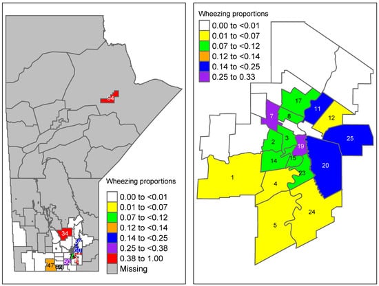
Figure 2.
Raw proportion of wheezing severity obtained from the data in Manitoba (aggregated wheezing severity at 3 months divided by sample size in each area). Winnipeg-specific proportions are shown on the right panel (region codes are given in Table A2).
The results of the final area-level ZIP (after model building steps) are reported in Table 4. The area-level ZIP model used maternal asthma and farm as covariates for both the logit (excess zero) and Poisson component, and thus did not use a prior for the excess zero component of the model. The area-level ZIP model indicated that living within a 100 m from a farm decreased the expected rate of wheezing episodes by 3%, while prenatal maternal asthma increased the expected rate of wheezing episodes by 1%.
Table 4.
Final area-level ZIP model.
Using the results of Table 4, the predicted average number of wheezing episodes in each area k (=) was calculated using . These predicted average wheezing episodes were then mapped to their corresponding RHADs in Manitoba (Figure 3). For comparison purposes, the area-level wheezing episodes at 3 months obtained from the raw data were also mapped (Figure 4). The average number of wheezing episodes obtained directly from the data indicated that many areas have no or a small number of wheezing episodes. In particular, regions 27, 28, and 45 had no wheezing episodes while the smoothed predictions using the proposed new ZIP model (Figure 3) had at least four episodes of wheezing in those areas.
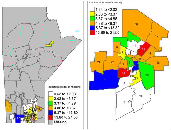
Figure 3.
Predicted average number of wheezing episodes in Manitoba using the final area-level (new) ZIP model. Winnipeg-specific proportions are shown on the right panel (region codes are given in Table A2).
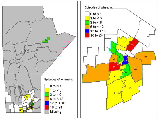
Figure 4.
Raw number of wheezing episodes obtained from the data in Manitoba (aggregated wheezing episodes at 3 months). Winnipeg-specific proportions are shown on the right panel (region codes are given in Table A2).
5. Discussion
The use of advanced statistical modeling techniques, particularly small area estimation (SAE) models, has proven to be valuable in this study. The application of Bayesian methods to both area-level and unit-level data has allowed for a more nuanced understanding of childhood wheezing patterns across Manitoba.
The simulation studies revealed that the proposed models performed well in terms of bias and the mean squared error (MSE) of the model parameter estimates. One of the key strengths of this study is the rigorous model validation process, including the use of the Gelman–Rubin diagnostic for ensuring MCMC convergence and the DIC statistics for model comparison. These steps have ensured that the models used are both statistically sound and robust. The choice of the hierarchical Bayesian approach provided flexibility in modeling the complex structure of the data, accommodating both individual and area-level random effects. We have selected non-informative priors within the models to prioritize data-driven influence over subjective bias.
The inclusion of auxiliary variables, such as maternal health history and environmental factors, has enhanced the precision of the estimates. These variables have acted as significant predictors, explaining a substantial portion of the variation in wheezing outcomes. The models demonstrated that maternal asthma and smoking are crucial risk factors, significantly increasing the odds and rates of wheezing in children.
Given the sparsity of the population in many regions of Manitoba, the use of SAE models was particularly appropriate. These models effectively drew strength from related areas, improving the estimates in regions with small sample sizes. This methodological approach is crucial for public health research in sparsely populated areas, ensuring that findings are reliable and actionable. As a practical guideline, we recommend using the proposed ordinal logistic model (Section 3.1) for longitudinal data with ordinal outcomes when the goal is to predict outcomes at the area level. Similarly, we suggest the proposed ZIP model (Section 3.3) for longitudinal count data with many zeros, with the same area-level prediction objective.
The implementation of the ZIP model addressed the issue of overdispersion and excess zeros in the count data of wheezing episodes. This model differentiated between children who never wheezed and those who did, providing a more accurate representation of the data. The ZIP model’s findings regarding the influence of environmental factors, such as proximity to farms, have important implications for understanding the triggers of wheezing in susceptible populations.
Notably, we encountered complex computational challenges in analyzing longitudinal data, particularly with high-dimensional covariates/areas and relatively small sample sizes. The interaction between these factors posed significant obstacles to achieving robust and efficient analytical methods. To overcome these difficulties, we leveraged high-performance computing resources to address computational constraints and employed small area estimation techniques to mitigate issues related to sample size limitations.
6. Conclusions
The methodological rigor applied in this study highlights several key findings and their implications for public health policy:
The study underscores the critical role of maternal health, particularly asthma and smoking, in influencing wheezing outcomes in children. These findings highlight the need for targeted interventions aimed at improving maternal health as a strategy to reduce childhood wheezing and asthma.
The use of Bayesian SAE models has provided more accurate and reliable estimates of wheezing prevalence and severity across Manitoba. These models are particularly valuable for public health surveillance in regions with sparse populations, offering insights that would not be possible with traditional methods.
The study has revealed the dual role of environmental factors, such as farm proximity, in influencing wheezing outcomes. While farm living appears to reduce the odds of developing wheezing, it increases the frequency of episodes among those already affected. These nuanced findings can inform targeted public health interventions and policies.
The study highlights the potential for further research using more comprehensive and longitudinal data. Future studies could expand on this work by incorporating additional environmental and genetic factors, as well as exploring the long-term impacts of early childhood wheezing on asthma development.
These innovative techniques can also be applied across different provinces and regions to examine variations in asthma and wheezing over both geographic areas and time.
Author Contributions
Conceptualization, methodology, software, resources, validation, visualization, formal analysis, investigation, data curation, writing—original draft preparation, writing—review and editing, C.S.; Conceptualization, methodology, validation, supervision, writing—review and editing, M.T. All authors have read and agreed to the published version of the manuscript.
Funding
This research received no specific grant from any funding agency in the public, commercial, or not-for-profit sectors.
Institutional Review Board Statement
The study was conducted in accordance with the Declaration of Helsinki and approved by the Health Research Ethics Board (HREB) of the University of Manitoba, with ethics number HS23359 (H2019:429). The approval was granted on 28 October 2024, and is valid until 15 November 2025. The project, titled “Modelling Severity of Wheezing in Small Areas in Manitoba Using Longitudinal Data”, underwent annual review and was found to be ethically acceptable for research involving human participants.
Informed Consent Statement
Informed consent was obtained from all subjects involved in the study.
Data Availability Statement
The dataset used in this study cannot be shared publicly due to copyright and privacy concerns for participants involved in the CHILD Cohort Study. For more details on data access policies, please visit https://childstudy.ca/for-researchers/data-access/ (accessed on 25 March 2025). The study utilized individual-level participant data, which are classified as controlled access.
Acknowledgments
We are very grafeful to Elinor Simons and Zeinab Mashreghi for their help in guiding and focusing the clinical and statistical objectives of this paper throughout multiple revisions and rewrites. We also sincerely thank the three reviewers for their constructive and insightful comments, which have significantly enhanced the quality and clarity of this manuscript. We thank the CHILD Cohort Study (CHILD) participant families for their dedication and commitment to advancing health research. CHILD was initially funded by CIHR and AllerGen NCE. Visit CHILD at childstudy.ca.
Conflicts of Interest
The authors declare that there are no conflicts of interest.
Appendix A. Supplementary Tables
Table A1.
Severity of wheezing frequency distribution for six follow-ups within the CHILD cohort. Scale of 0–3, 0 being no evidence of wheezing.
Table A1.
Severity of wheezing frequency distribution for six follow-ups within the CHILD cohort. Scale of 0–3, 0 being no evidence of wheezing.
| Severity of Wheezing | ||||||
|---|---|---|---|---|---|---|
| Severity | 3 Months | 6 Months | 1 Year | 18 Months | 2 Years | 2.5 Years |
| 0 | 618 | 596 | 576 | 567 | 600 | 581 |
| 1 | 34 | 29 | 26 | 2 | 31 | 24 |
| 2 | 19 | 16 | 19 | 6 | 17 | 12 |
| 3 | 8 | 7 | 12 | 2 | 13 | 9 |
| Missing | 11 | 42 | 57 | 112 | 29 | 64 |
Table A2.
Region code with associated location and small area number.
Table A2.
Region code with associated location and small area number.
| Code | Region | Small Area |
|---|---|---|
| W002 | Assiniboine South | 1 |
| W11A | Downtown | 2 |
| W11B | Downtown | 3 |
| W03A | Ft. Garry | 4 |
| W03B | Ft. Garry | 5 |
| W09A | Inkster | 6 |
| W09B | Inkster | 7 |
| W10A | Point Douglas | 8 |
| W10B | Point Douglas | 9 |
| W07A | River East | 10 |
| W07B | River East | 11 |
| W07C | River East | 12 |
| W07D | River East | 13 |
| W12A | River Heights | 14 |
| W12B | River Heights | 15 |
| W08A | Seven Oaks | 16 |
| W08B | Seven Oaks | 17 |
| W08C | Seven Oaks | 18 |
| W05A | St. Boniface | 19 |
| W05B | St. Boniface | 20 |
| W01A | St. James-Assiniboia | 21 |
| W01B | St. James-Assiniboia | 22 |
| W04A | St. Vital | 23 |
| W04B | St. Vital | 24 |
| W006 | Transcona | 25 |
| WE34 | Souris River | 26 |
| WE31 | Asessippi | 27 |
| WE36 | Spruce Woods | 28 |
| IE42 | Arborg/Riverton | 29 |
| WE32 | Little Saskatchewan | 30 |
| IE31 | Beausejour | 31 |
| WE33 | Turtle Mountain | 32 |
| SO14 | Cartier/SFX | 33 |
| IE43 | St. Laurent | 34 |
| WE13 | Riding Mountain | 35 |
| WE15 | Dauphin | 36 |
| SO25 | St Pierre/DeSalaberry | 37 |
| SO22 | Carman | 38 |
| SO26 | Red River South | 39 |
| IE41 | Gimli | 40 |
| WE35 | Whitemud | 41 |
| WE11 | Duck Mountain | 42 |
| SO45 | Hanover | 43 |
| SO44 | Steinbach | 44 |
| IE32 | Pinawa/LDB | 45 |
| SO11 | Seven Regions | 46 |
| SO31 | Lorne/Louise/Pembina | 47 |
| SO23 | MacDonald | 48 |
| WE12 | Porcupine Mountain | 49 |
| SO24 | Morris | 50 |
| SO12 | MacGregor | 51 |
| SO13 | Rural Portage | 52 |
| SO15 | City of Portage la Prair | 53 |
| SO33 | Altona | 54 |
| IE21 | Stonewall/Teulon | 55 |
| SO36 | Roland/Thompson | 56 |
| IE22 | Wpg Beach/St. Andrews | 57 |
| IE11 | Selkirk | 58 |
| IE23 | St. Clements | 59 |
| IE24 | Springfield | 60 |
| SO32 | Stanley | 61 |
| SO34 | Morden | 62 |
| SO35 | Winkler | 63 |
| SO42 | Tache | 64 |
| WP21 | Winnipeg Churchill | 65 |
| IE52 | Fisher/Peguis | 66 |
| NO11 | Flin, Snow, Cran, Sher | 67 |
| NO13 | LL/MC, LR, O-P(SIL), PN(GVL) | 68 |
| IE51 | Powerview/PF | 69 |
| NO21 | GR/Mis, ML/Mos, Eas/Che | 70 |
| SO43 | Ste Anne/LaBroquerie | 71 |
| SO21 | Nortre Dame/St. Claude | 72 |
| NO14 | Thomp, Myst Lake | 73 |
| SO41 | Niverville/Richot | 74 |
| IE61 | Northern Remote | 75 |
| SO46 | Rural East | 76 |
| NO22 | Puk/Mat Col CN | 77 |
| NO23 | SayD(TL), Bro/BL, NoL(Lac) | 78 |
| NO26 | Bu(OH), MS(GR), GLN/GLFN | 79 |
| NO28 | Norway House/NH CN | 80 |
| NO27 | Cross Lake/Pimi CN | 81 |
| NO31 | Island Lake | 82 |
| IE33 | Whiteshell | 83 |
| WE14 | Agassiz Mountain | 84 |
| WE16 | Swan River | 85 |
| WE23 | Bdn Downtown | 86 |
| WE24 | Bdn South End | 87 |
| WE22 | Bdn North Hill | 88 |
| WE25 | Bdn East End | 89 |
| WE21 | Bdn West End | 90 |
| IE53 | Eriksdale/Ashern | 91 |
| NO12 | The Pas/OCN, Kels | 92 |
| NO15 | Bay Line | 93 |
| NO16 | Gillam, Fox Lake CN | 94 |
| NO25 | Sham, YorkF, Tat(SPL) | 95 |
| NO24 | Nelson House/NCN | 96 |
Appendix B. Simulation Studies: Theory and Results
Appendix B.1. Ordinal Logistic Model
A simulation study was performed in which data were simulated with an ordinal response; the response represented the wheezing severity scale found on the CHILD study questionnaires. The dependent variable or response variable was randomly generated with 1600 random values, all ranging from 1–3 using the integer uniform distribution or trinomial distribution. The probability of generating each integer was ; thus, equal probabilities. The aim of the simulation was to investigate the performance of the proposed ordinal logistic model with a similar set-up as the data structure from the CHILD cohort. The ordinal logistic model used for the simulation is described as follows. Let have three levels ; thus, there were two categories (with another level as a reference category). We then obtain
where i represents the individual, j is follow-up, and k is small area, and
Thus, the two logit equations with are
For the simulation, there were 20 individuals, 4 follow-ups, and 20 small areas. The covariates , , and were generated from a binary distribution with the probability of generating each integer being equal to . The simulation was conducted by fitting the simulated data with the ordinal logistic model using Rjags. Diffuse priors were used for all the model parameters. Coefficients from the fitted model were then to be used as true parameters, since a starting point was needed to begin the simulations.
These estimates were then used as the true parameters for the simulation study. The initial goal was to evaluate the performance of the model parameters. The simulation procedure was as follows:
Algorithm A
- Step 1:
- Consider the estimates from Table A3 as the true parameters, represented by the vector
- Step 2:
- Use the true parameters to generate the random effects, which, in turn, generate the new response values
- Step 3:
- Refit the model using the new generated response values
- Step 4:
- Extract the estimates from the newly fitted model
- Step 5:
- Repeat the cycle by going to step 2
Table A3.
Ordinal Simulation Study: Three chains are used with 60,000 samples from each chain. Furthermore, the Gelman diagnostics indicated convergence of model parameters. These estimates were used as the true parameters for the ordinal logistic model.
Table A3.
Ordinal Simulation Study: Three chains are used with 60,000 samples from each chain. Furthermore, the Gelman diagnostics indicated convergence of model parameters. These estimates were used as the true parameters for the ordinal logistic model.
| Parameter | Estimate |
|---|---|
| −0.685 | |
| 0.772 | |
| −0.090 | |
| 0.068 | |
| 0.170 | |
| 0.378 | |
| 0.145 | |
| 0.162 | |
| 0.169 |
In the above steps, the model was essentially reversed in the sense that the aim was to simulate values of the response using the ordinal model described before and thus replacing the original values of with the simulated values of and then refitting the same ordinal model; this was performed 500 times. Each simulation run produced its own estimates () of the model parameters. Then, the bias, relative bias (R. Bias), and MSE (Mean Square Error) were calculated using the three formulas below, assuming element-wise operation of the vectors. The bias and relative bias were used to quantify the average difference between the true parameters and the estimates within the simulations runs. The MSE was used to assess, on average, how far an estimator was from the true parameter within the simulation runs.
The results from Table A4 indicated the model parameter estimates have very small bias and MSE. The relative bias for is higher than the other parameters, but overall it is acceptable. A possible explanation is that the number of small areas may not have been enough in this simulation set-up to reflect the performance of small area variation in the proposed model. Thus, the results indicate that the estimated parameters are working well in the proposed model.
Table A4.
Bias, relative bias (R. Bias), and MSE of model parameter estimates based on 500 simulation runs from the proposed ordinal logistic model.
Table A4.
Bias, relative bias (R. Bias), and MSE of model parameter estimates based on 500 simulation runs from the proposed ordinal logistic model.
| Parameter | True | Bias | R. Bias (%) | MSE |
|---|---|---|---|---|
| −0.685 | −0.022 | 3.21 | 0.037 | |
| 0.772 | 0.010 | 1.24 | 0.038 | |
| −0.090 | 0.003 | −3.33 | 0.011 | |
| 0.068 | −0.002 | −2.94 | 0.009 | |
| 0.170 | −0.010 | −5.88 | 0.009 | |
| 0.378 | −0.019 | −4.95 | 0.015 | |
| 0.145 | 0.028 | 19.24 | 0.015 | |
| 0.162 | 0.011 | 6.48 | 0.001 | |
| 0.169 | −0.006 | −3.55 | 0.001 |
Further simulation studies were performed, which assumed the responses are binary and count; thus, logit and log link functions were used.
Appendix B.2. Binary Logistic Model
The model is described as
where is the response of wheezing for individual i, follow-up j, and small area k. Then, is the probability that the individual i had a wheezing event at follow-up j, and in small area k. Now the logistic model is described as
where
Now, is the random effect of the individual and follow-up. Usually, this is the time-specific disturbance, but in the case of this model, the disturbance is an autoregressive-one or AR(1) model and is simply the random effect of each small area. A simulation study was performed in which data were simulated with a binary response; the response represented whether each child within the cohort wheezed or not. The aim of the simulation was to verify the estimates produced by a binary logistic model with data representing the CHILD cohort. For the simulation, there were 20 individuals, 4 follow-ups, and 20 small areas. The dependent variable was randomly generated with 1600 random binary values from a Bernoulli distribution. The probability of generating each integer was ; thus, equal probabilities. The covariates ,, and were also generated from a binary distribution with the probability of generating each integer being equal to . The estimated parameters are reported in Table A5.
Table A5.
Binary Logistic Simulation Study: Three chains were used, with 60,000 samples from each chain. Furthermore, the Gelman diagnostics indicated convergence of model parameters. These estimates were used as the true parameters for the binary logistic model.
Table A5.
Binary Logistic Simulation Study: Three chains were used, with 60,000 samples from each chain. Furthermore, the Gelman diagnostics indicated convergence of model parameters. These estimates were used as the true parameters for the binary logistic model.
| Parameter | Estimate |
|---|---|
| −0.298 | |
| −0.118 | |
| 0.270 | |
| 0.0168 | |
| 0.0117 | |
| 0.111 | |
| 0.128 |
The goal was to evaluate the performance of the model parameters in the proposed logistic model. The simulation procedure followed from Algorithm A. In the simulation steps, the model was essentially reversed in the sense that the aim was to simulate the values of the response using the binary logistic model described before, thus replacing the original values of with the simulated values of and then refitting the same binary logistic model; this was performed 500 times. Each simulation run produced its own estimates () of the model parameters. Then, the bias, relative bias (R. Bias), and MSE were calculated (Table A6).
The results from Table A6 indicated the model parameter estimates had small bias and MSE. The relative bias for was higher than the other parameters, but it was still acceptable. Note that the model is sensitive to the number of follow-ups in the dataset. Ultimately, the number of areas, follow-ups and individuals chosen show how well the simulation performed. Thus, the overall results indicated that the estimated parameters were working well in the proposed binary logistic model.
Table A6.
Bias, relative bias (R. Bias), and MSE of model parameter estimates based on 500 simulation runs from the proposed binary logistic model.
Table A6.
Bias, relative bias (R. Bias), and MSE of model parameter estimates based on 500 simulation runs from the proposed binary logistic model.
| Parameter | True | Bias | R. Bias (%) | MSE |
|---|---|---|---|---|
| −0.298 | 0.009 | −3.00 | < | |
| −0.118 | −0.002 | −1.80 | < | |
| 0.270 | −0.001 | -0.41 | < | |
| 0.0168 | −0.0002 | −8.40 | < | |
| 0.0117 | 0.0025 | 22.70 | < | |
| 0.111 | 0.0005 | 0.47 | < | |
| 0.128 | 0.0006 | 0.62 | < |
Appendix B.3. Zero-Inflated Poisson Model
We also simulated the Zero-Inflated Poisson (ZIP) model, in which the response was the number of wheezing episodes for each child in the cohort. We considered the same covariates as discussed in the previous logistic model (Appendix B.2). For this simulation, we were less interested in the modeling of false zeros; therefore, a diffuse prior for was implemented such that , . Again, for the simulation, there were 20 individuals, 4 follow-ups, and 20 small areas. The dependent variable was randomly generated with 1600 random values from the ZIP distribution with and , which give the range of possible values for as between 0 and 13. The covariates , , and were also generated from a binary distribution with the probability of generating each integer being equal to . The statistical measures used to test the credibility of the models were the bias and MSE. Now, let
where
Then, the ZIP model becomes,
such that and where .
The model parameter estimates are presented in Table A7. Then, the simulation procedure follows Algorithm A. Similar to previous simulations, the model was essentially reversed. Each simulation run produced its own estimates () of the model parameters. Then, the bias, relative bias (R. Bias), and MSE were calculated (Table A8).
The results from Table A8 indicate that the model parameter estimates behaved reasonably well; however, some parameters had relative bias above 30 percent, which, after further investigation, was due to not being statistically significant for this particular simulated dataset. When using such a model with real data, particular attention should be placed on the AR(1) and this should be removed if not significant.
Table A7.
ZIP Simulation Study: Three chains are used with 60,000 samples from each chain. Furthermore, the Gelman diagnostics indicated convergence of model parameters. These estimates are to be used as the true parameters for the ZIP model.
Table A7.
ZIP Simulation Study: Three chains are used with 60,000 samples from each chain. Furthermore, the Gelman diagnostics indicated convergence of model parameters. These estimates are to be used as the true parameters for the ZIP model.
| Parameter | Estimate |
|---|---|
| 1.085 | |
| −0.034 | |
| 0.066 | |
| 0.085 | |
| −0.304 | |
| 0.657 | |
| 0.575 | |
| 0.639 | |
| 0.042 |
Table A8.
Bias, relative bias (R. Bias), and MSE of model parameter estimates based on 500 simulation runs from the proposed ZIP model.
Table A8.
Bias, relative bias (R. Bias), and MSE of model parameter estimates based on 500 simulation runs from the proposed ZIP model.
| Parameter | True | Bias | R. Bias (%) | MSE |
|---|---|---|---|---|
| 1.085 | 0.270 | 24.9 | 0.252 | |
| −0.034 | −0.003 | 8.40 | < | |
| 0.066 | 0.002 | 3.30 | < | |
| 0.085 | -0.003 | −3.50 | < | |
| −0.304 | < | 0.10 | < | |
| 0.657 | −0.224 | −34.10 | 0.194 | |
| 0.575 | < | < | < | |
| 0.639 | −0.210 | −34.00 | 0.355 | |
| 0.042 | < | 0.30 | < |
References
- Global Initiative for Asthma. Global Strategy for Asthma Management and Prevention. Eur. Respir. J. 2008, 31, 143–178. [Google Scholar] [CrossRef] [PubMed]
- Public Health Agency of Canada. Report from the Canadian Chronic Disease Surveillance System: Asthma and Chronic Obstructive Pulmonary Disease (COPD) in Canada, 2018; Public Health Agency of Canada: Ottawa, ON, Canada, 2018.
- Statistics Canada. Table 13-10-0096-08 Asthma, by Age Group, 2022. [CrossRef]
- Nahum, U.; Gorlanova, O.; Decrue, F.; Oller, H.; Delgado-Eckert, E.; Böck, A.; Schulzke, S.; Latzin, P.; Schaub, B.; Karvonen, A.M.; et al. Symptom trajectories in infancy for the prediction of subsequent wheeze and asthma in the BILD and PASTURE cohorts: A dynamic network analysis. Lancet Digit. Health 2024, 6, e718–e728. [Google Scholar] [CrossRef] [PubMed]
- Rao, J.; Molina, I. Small Area Estimation; John Wiley & Sons, Ltd.: Hoboken, NJ, USA, 2015. [Google Scholar] [CrossRef]
- Richelle, J. Wheezing in Early Life and Validating the Asthma Predictive Index. Bachelor Thesis, University of Manitoba, Winnipeg, MB, Canada, 2014. [Google Scholar]
- Jiang, J.; Torabi, M. Sumca: Simple, unified, Monte-Carlo-assisted approach to second-order unbiased mean-squared prediction error estimation. J. R. Stat. Soc. Ser. B 2020, 82, 467–485. [Google Scholar] [CrossRef]
- Torabi, M.; Lele, S.R.; Prasad, N.G. Likelihood inference for small area estimation using data cloning. Comput. Stat. Data Anal. 2015, 89, 158–171. [Google Scholar] [CrossRef]
- Battese, G.E.; Harter, R.M.; Fuller, W.A. An error-components model for prediction of county crop areas using survey and satellite data. J. Am. Stat. Assoc. 1988, 83, 28–36. [Google Scholar] [CrossRef]
- Fay, R.E.; Herriot, R.A. Estimates of Income for Small Places: An Application of James-Stein Procedures to Census Data. J. Am. Stat. Assoc. 1979, 74, 269–277. [Google Scholar] [CrossRef]
- Alkan, N. Assessing convergence diagnostic tests for Bayesian Cox regression. Commun. Stat. Simul. Comput. 2017, 46, 3201–3212. [Google Scholar] [CrossRef]
- Chan, J.C.C.; Grant, A.L. On the Observed-Data Deviance Information Criterion for Volatility Modeling. J. Financ. Econom. 2016, 14, 772–802. [Google Scholar] [CrossRef]
- Torabi, M.; Shokoohi, F. Likelihood inference in small area estimation by combining time-series and cross-sectional data. J. Multivar. Anal. 2012, 111, 213–221. [Google Scholar] [CrossRef]
- Torabi, M.; Shokoohi, F. Hierarchical Bayes estimation in small area estimation using cross-sectional and time-series data. J. Stat. Comput. Simul. 2014, 84, 605–613. [Google Scholar] [CrossRef]
- Shokoohi, F.; Torabi, M. Semi-parametric small-area estimation by combining time-series and cross-sectional data methods. Aust. N. Z. J. Stat. 2018, 60, 323–342. [Google Scholar] [CrossRef]
- Torabi, M. Zero-inflated spatio-temporal models for disease mapping. Biom. J. 2017, 59, 430–444. [Google Scholar] [CrossRef] [PubMed]
Disclaimer/Publisher’s Note: The statements, opinions and data contained in all publications are solely those of the individual author(s) and contributor(s) and not of MDPI and/or the editor(s). MDPI and/or the editor(s) disclaim responsibility for any injury to people or property resulting from any ideas, methods, instructions or products referred to in the content. |
© 2025 by the authors. Licensee MDPI, Basel, Switzerland. This article is an open access article distributed under the terms and conditions of the Creative Commons Attribution (CC BY) license (https://creativecommons.org/licenses/by/4.0/).