A Flexible Bivariate Integer-Valued Autoregressive of Order (1) Model for Over- and Under-Dispersed Time Series Applications

Abstract

In real-life inter-related time series, the counting responses of different entities are commonly influenced by some time-dependent covariates, while the individual counting series may exhibit different levels of mutual over- or under-dispersion or mixed levels of over- and under-dispersion. In the current literature, there is still no flexible bivariate time series process that can model series of data of such types. This paper introduces a bivariate integer-valued autoregressive of order 1 (BINAR(1)) model with COM-Poisson innovations under time-dependent moments that can accommodate different levels of over- and under-dispersion. Another particularity of the proposed model is that the cross-correlation between the series is induced locally by relating the current observation of one series with the previous-lagged observation of the other series. The estimation of the model parameters is conducted via a Generalized Quasi-Likelihood (GQL) approach. The proposed model is applied to different real-life series problems in Mauritius, including transport, finance, and socio-economic sectors.

1. Introduction

In real-life series applications, it is commonly seen that the current observation in a counting process is influenced by the previous-lagged observation of another related series. Likewise, a popular example in the literature is the tick by tick data from the New York Stock Exchange (NYSE) market that concerns the trading intensity of stocks from different competing firms. Specifically, Pedeli and Karlis [1] referred to the intraday bid and ask quotes of AT&T stock on the NYSE market where these researchers remarked that the fluctuation in the investment level of intraday bid quotes of AT&T at a specified time point was affected by the transaction level of the ask quotes of AT&T at the previous time point. Similar scenarios of this nature can be encountered in different real-life socio-economic instances such as in time series related to day and night accidents over a same area or the number of thefts or larceny cases and unemployed people in a populated region. The analysis of such series of data poses a number of challenges. Firstly, both series are commonly influenced by some dynamic time-variant factors that lead to time-changing moments and correlations. Secondly, the series are often subject to different levels of over-, under-, or mixed-dispersion. From the papers published in this field of research [1,2,3,4,5,6], there is yet no bivariate time series process that accommodates for the mixed-dispersion of a wider range under non-stationary conditions based on the cross-correlation design specified above.

However, under a simpler cross-correlation design, Jowaheer et al. [7] have most recently proposed a bivariate integer-valued autoregressive process of order 1 (BINAR(1)M1) with COM-Poisson innovations featured under time-dependent moments that were induced through dynamic explanatory variables. The COM-Poisson is a discrete distribution re-introduced by Shmueli et al. [8] that can model a wider range of over- and under-dispersion and has shown its capability in different univariate areas of application (see Lord et al. [9,10], Sellers and Shmueli [11], Nadarajah [12], Zhu [13], Guikema and Coffelt [14], Borle [15,16,17]). This BINAR(1)M1 was a simple extension of the classical INAR(1)-based binomial thinning process of McKenzie [18]. Jowaheer et al. [7] extended by assuming two INAR(1) series with COM-Poisson innovations where the cross-correlation was simply sourced from the correlated COM-Poisson innovations similar to the bivariate design proposed initially by Pedeli and Karlis [19,20], Karlis and Pedeli [21], and later by Mamode Khan et al. [22]. For this non-stationary BINAR(1)M1 process, Jowaheer et al. [7] showed, through Monte Carlo experiments, that the model can be effectively used to simulate and represent real-life experiments where different quantities of over-or under-dispersed or mixed-dispersed series of data are collected. However, as remarked, the local inter-relationship between cross-related observations of same and previous lags as depicted in the stock example above is ignored.

In the literature, another class of BINAR(1) models (BINAR(1)M2) has been developed to cater for the possible relationship between current counting series observation with previous-lagged other series observations. Pedeli and Karlis [1] proposed such a BINAR(1)M2 with correlated Poisson innovations where the source of inter-relationship was induced by the cross-related observations and the bivariate Poisson innovations [23]. In this model construction, the counting series was marginally found to follow a Hermite distribution and hence this model was appropriate for series exhibiting mutually mild over-dispersion of different quantum. However, these two sources of cross-correlation increase the number of parameters to be estimated and complicate the specification of the conditional likelihood. Another less complicated version of BINAR(1)M2 (BINAR(1)M3) was proposed by Ristic et al. [2] and Nastic et al. [3] where these authors assumed that the cross-correlation could be simply induced by relating the current series observation with the previous-lagged observation of the other series with the pair of innovations held independently. Ristic et al. [2] and Nastic et al. [3] developed the BINAR(1)M3 with geometric marginal based on the Negative Binomial (NB) thinning mechanism, which indicates that BINAR(1)M3 was only suited for modeling a series of restricted levels of over-dispersion. Interestingly, Nastic et al. [3] showed that this BINAR(1)M3 provides better Akaike information criterion (AICs) and root mean square error (RMSE) than the BINAR(1)M1 with NB innovations by Karlis and Pedeli [21] and BINAR(1)M2 with Poisson innovations by Pedeli and Karlis [1]. Overall, BINAR(1)M2 and BINAR(1)M3 were developed under stationary conditions only and lack the flexibility to model situations of varied levels of dispersion under set-ups comprising time-independent and time-dependent covariates. This paper aims at developing a versatile non-stationary BINAR(1) model of similar structure as BINAR(1)M3 with COM-Poisson innovations but under binomial thinning that could accommodate the different scenarios of dispersion, as well as the influence of the current series-counting observation by the previous-lagged observation of another series.

As for the inferential procedures, Conditional Maximum Likelihood Estimation (CMLE) and Least Squares (LS) techniques have been mostly used to estimate the unknown model parameters in the existing stationary BINAR(1)M1, BINAR(1)M2, and BINAR(1)M3 models [1,2,3,19,20]. Nastic et al. [3] demonstrated that CMLE and LS asymptotically yield estimates of almost the same level of efficiency, but LS is less computationally intensive. The computational cumbersomeness of CMLE was also discussed by Pedeli and Karlis [24] where the authors noticed that under bivariate time series modeling, the implementation of CMLE is not quite feasible due to the intensive Hessian entries. As for the non-stationary BINAR(1)M1 developed by Mamode Khan et al. [22] with Poisson innovations, it was seen that the specification of the conditional likelihood function was rather tedious, and alternatively, they developed a novel Generalized Quasi-Likelihood (GQL) estimator that depends only on the correct specification of the mean scores. The other components of GQL are the derivatives and auto-covariance structure. As for the auto-covariance specification, this was computed in its exact form using the auto-regressive structure but with the correlation parameters estimated by the method of moments. Mamode Khan et al. [22] prove that both GQL and CMLE yield estimates with an asymptotic level of efficiency (see also Sutradhar et al. [25]) but remarkably, GQL yields considerably fewer non-convergent simulations. In similar lines, Sunecher et al. [26] compared LS with GQL for bivariate integer-valued moving-average of order 1 (BINMA(1)) process. wherein GQL provides more superior efficient estimates than LS with fewer non-convergent failures. Thus, in this paper, we consider formulating a new GQL method since the bivariate auto-correlation structure is different from the BINMA(1) process.

The organization of the paper is as follows: In Section 2, the new BINAR(1) model with COM-Poisson innovations is constructed and its properties are derived. Prior to this, we outline the basics of the COM-Poisson model. In Section 3, the GQL algorithm is implemented to estimate the regression, dispersion, and serial- and cross-dependence parameters. In Section 4, we present some numerical experiments to illustrate the different scenarios of over, under, and mixed dispersion under various combinations of the serial- and cross-correlation parameters. 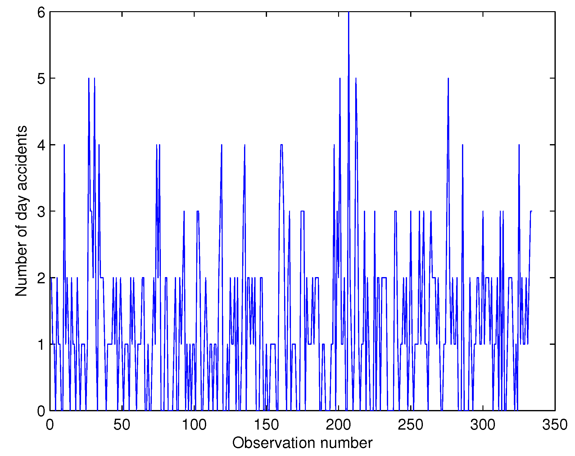In Section 5, the model is applied to three real-life time series data in Mauritius: Firstly, the model is employed in analyzing series of daily day and night accidents on the motorway from the International Airport in Mauritius to the northern zone Grand Bay from 1 February to 30 November 2015. In the second instance, it is applied to the time series of intra-day transactions of two competing banks operating on the Stock Exchange of Mauritius (SEM) from 3 August 2015 to 12 October 2015. The third application consists of analyzing a socio-economic problem of the daily day and night frequently occurring thefts in the Capital City of Port Louis from 1 January to 30 November 2015. This paper ends with some concluding remarks in Section 6.

2. Model Development

Suppose that the BINAR(1) model $\{[Y_t^{\left[1\right]},Y_t^{\left[2\right]}{]}^{\prime },t\in \mathbb{Z}\}$ is of the form

$$\left(\begin{array}{c}{Y}_t^{\left[1\right]}\\ Y_t^{\left[2\right]}\end{array}\right)=\left(\begin{array}{cc}{\rho }_{11}& {\rho }_{12}\\ {\rho }_{21}& {\rho }_{22}\end{array}\right)\circ \left(\begin{array}{c}{Y}_{t-1}^{\left[1\right]}\\ Y_{t-1}^{\left[2\right]}\end{array}\right)+\left(\begin{array}{c}{R}_t^{\left[1\right]}\\ R_t^{\left[2\right]}\end{array}\right)$$

(1)

where ‘∘’ indicates the binomial thinning operator [27], wherein ${\rho }_{jk}\circ Y_{t-1}^{\left[k\right]}$, for

$${\rho }_{jk}\circ Y_{t-1}^{\left[k\right]}=\left\{\begin{array}{cc}\sum _{l=1}^{Y_{t-1}^{\left[k\right]}}{b}_l\left({\rho }_{jk}\right),\hfill & Y_{t-1}^{\left[k\right]}>0,\hfill \\ 0\hfill & Y_{t-1}^{\left[k\right]}=0\hfill \end{array}\right.$$

(2)

and the so-called counting $\left\{b_l\left({\rho }_{jk}\right)\right\}$ is a sequence of independent and identically distributed Bernoulli random variable with P$\left\{b_l\left({\rho }_{jk}\right)\right\}=1-\mathrm{P}\left\{b_l\left({\rho }_{jk}\right)\right\}={\rho }_{jk}$, for ${\rho }_{jk}\in [0,1]$.

$R_t^{\left[1\right]}$ and $R_t^{\left[2\right]}$ are the corresponding innovation terms for $Y_t^{\left[1\right]}$ and $Y_t^{\left[2\right]}$, respectively, and $R_t^{\left[k\right]}$, $k\in \{1,2\}$ is marginally COM-Poisson with probability function

$$P(R_t^{\left[k\right]}=r_k)={\displaystyle \frac{{\left({\theta }_t^{\left[k\right]}\right)}^{r_k}}{{(r_k!)}^{{\nu }_k}}}{\displaystyle \frac{1}{Z({\theta }_t^{\left[k\right]},{\nu }_k)}},r_k=0,1,2,3,\cdots ,\mathrm{for}{\theta }_t^{\left[k\right]}>0,{\nu }_k\ge 0,k\in \{1,2\}.$$

(3)

2.1. Properties of the COM-Poisson Model

In the above, $Z({\theta }_t^{\left[k\right]},{\nu }_k)={\sum }_{j=0}^{\infty }{\displaystyle \frac{{{\theta }_t^{\left[k\right]}}^j}{{(j!)}^{{\nu }_k}}}$. The COM-Poisson model (3) generalizes several discrete distributions. Likewise, under ${\nu }_k=0$ and ${\theta }_t^{\left[k\right]}<1$, the geometric distribution becomes a special case of the COM-Poisson. Under ${\nu }_k=1$, it generalizes the Poisson distribution with mean parameter ${\theta }_t^{\left[k\right]}$ and becomes Bernoulli when ${\nu }_k\to \infty$ with the probability of success given by ${\displaystyle \frac{{\theta }_t^{\left[k\right]}}{1+{\theta }_t^{\left[k\right]}}}$. Under any parametrization of ${\theta }_t^{\left[k\right]}$ and ${\nu }_k$, the COM-Poisson is shown to be a member of the exponential family with link predictor function $ln{\theta }_t^{\left[k\right]}={\mathit{x}}_t^{\prime }{\mathit{\beta }}^{\left[k\right]}$ for ${\mathit{x}}_t=[x_{t1},x_{t2},\cdots ,x_{tj},\cdots ,x_{tp}{]}^{\prime }$ and ${\mathit{\beta }}^{\left[k\right]}=[{\beta }_1^{\left[k\right]},{\beta }_2^{\left[k\right]},\cdots ,{\beta }_j^{\left[k\right]},\cdots ,{\beta }_p^{\left[k\right]}{]}^{\prime }$. Furthermore, ${\nu }_k$ is regarded as the dispersion parameter such that ${\nu }_k>1$ represents under-dispersion and ${\nu }_k<1$ over-dispersion.

The moment generating function (mgf) and probability generating function (pgf) are expressed as

$$E\left[e^{R_t^{\left[k\right]}s}\right]={\displaystyle \frac{Z({\theta }_t^{\left[k\right]}{e}^s,{\nu }_k)}{Z({\theta }_t^{\left[k\right]},{\nu }_k)}}\mathrm{and}E\left[s^{R_t^{\left[k\right]}}\right]={\displaystyle \frac{Z({\theta }_t^{\left[k\right]}s,{\nu }_k)}{Z({\theta }_t^{\left[k\right]},{\nu }_k)}}.$$

(4)

while the moments of the COM-Poisson model are derived iteratively using

$$E\left({R_t^{\left[k\right]}}^{s+1}\right)=\left\{\begin{array}{cc}{\theta }_t^{\left[k\right]}E{(R_t^{\left[k\right]}+1)}^{1-{\nu }_k}\hfill & s=0,\hfill \\ \\ {\theta }_t^{\left[k\right]}{\displaystyle \frac{\mathsf{\partial }}{\mathsf{\partial }{\theta }_t^{\left[k\right]}}}E\left({R_t^{\left[k\right]}}^s\right)+E\left(R_t^{\left[k\right]}\right)E\left({R_t^{\left[k\right]}}^s\right)\hfill & s>0\hfill \end{array}\right.$$

(5)

In particular, the mean and variance are given as follows:

$$E\left(R_t^{\left[k\right]}\right)={\lambda }_t^{\left[k\right]}={\theta }_t^{\left[k\right]}{\displaystyle \frac{\mathsf{\partial }}{\mathsf{\partial }{\theta }_t^{\left[k\right]}}}\log Z({\theta }_t^{\left[k\right]},{\nu }_k)\mathrm{and}\mathrm{Var}\left(R_t^{\left[k\right]}\right)={{\sigma }_t^2}^{\left[k\right]}={\theta }_t^{\left[k\right]}{\displaystyle \frac{\mathsf{\partial }E\left(R_t^{\left[k\right]}\right)}{\mathsf{\partial }{\theta }_t^{\left[k\right]}}}.$$

(6)

However, these moments can be approximated in closed forms using the asymptotic approximation by Minka et al. [28]

$$Z({\theta }_t^{\left[k\right]},{\nu }_k)={\displaystyle \frac{exp\left({\nu }_k{{\theta }_t^{\left[k\right]}}^{1/{\nu }_k}\right)}{{\left(2\pi {{\theta }_t^{\left[k\right]}}^{1/{\nu }_k}\right)}^{\frac{{\nu }_k-1}{2}}\sqrt{{\nu }_k}}}[1+O\left({{\theta }_t^{\left[k\right]}}^{-1/{\nu }_k}\right)]$$

(7)

that yields

$${\lambda }_t^{\left[k\right]}\simeq {{\theta }_t^{\left[k\right]}}^{1/{\nu }_k}-{\displaystyle \frac{{\nu }_k-1}{2{\nu }_k}}\mathrm{and}{{\sigma }_t^2}^{\left[k\right]}\simeq {\theta }_t^{\left[k\right]}{\displaystyle \frac{\mathsf{\partial }}{\mathsf{\partial }{\theta }_t^{\left[k\right]}}}({{\theta }_t^{\left[k\right]}}^{1/{\nu }_k}-{\displaystyle \frac{{\nu }_k-1}{2{\nu }_k}})={\displaystyle \frac{{{\theta }_t^{\left[k\right]}}^{1/{\nu }_k}}{{\nu }_k}}$$

(8)

or alternatively, from Equation (8), ${{\sigma }_t^2}^{\left[k\right]}$ can be re-written as ${{\sigma }_t^2}^{\left[k\right]}\simeq {\displaystyle \frac{{\lambda }_t^{\left[k\right]}}{{\nu }_k}}+{\displaystyle \frac{{\nu }_k-1}{2{{\nu }_k}^2}}$ (see Mamode Khan and Jowaheer [29] and Mamode Khan [30]). Hence, under this parametrization, (${\lambda }_t^{\left[k\right]},{\nu }_k$) is the pair of parameters to describe the COM-Poisson variable $R_t^{\left[k\right]}$, such that $R_t^{\left[k\right]}\sim \mathrm{COM}\text{-}\mathrm{Poisson}({\lambda }_t^{\left[k\right]},{\nu }_k)$.

In the context of the above approximated moments, Minka et al. [28], Shmueli et al. [8], and Zhu [13] presented some trial experiments that reveal that these approximations are more accurate for large ${\theta }_t^{\left[k\right]}$. As also commented by Jowaheer et al. [7], for large ${\theta }_t^{\left[k\right]}$ and ${\nu }_k<1$, the Var($R_t^{\left[k\right]}$) outweighs the E($R_t^{\left[k\right]}$), while for large ${\theta }_t^{\left[k\right]}$ and ${\nu }_k>1$, for the COM-Poisson $R_t^{\left[k\right]}$, the E($R_t^{\left[k\right]})>$ Var($R_t^{\left[k\right]}$) indicates under-dispersion, but in fact for ${\nu }_k>1$, Nadarajah [12] provides an exact expression for the mean and variance based on generalized hypergeometric function. However, the approximation by Minka et al. [28] is rather more suitable as it explores the full range of ${\nu }_k\ge 0$.

Remark 1. 

From Equation (8), it is deduced that any increase/decrease in ${\theta }_t^{\left[k\right]}$ causes a similar change in ${\lambda }_t^{\left[k\right]}$. As for the magnitude of the change from $x_{tj}$ to $x_{tj}+1$ for $j=1,2,\cdots ,p$, the % change in ${\theta }_t^{\left[k\right]}$ is given by $[exp\left({\beta }_j^{\left[k\right]}\right)-1]\%$, while the % change in ${\lambda }_t^{\left[k\right]}$ is ${\displaystyle \frac{[exp({\beta }_j^{\left[k\right]}/{\nu }_k)-1]{{\theta }_t^{\left[k\right]}}^{1/{\nu }_k}}{{\lambda }_t^{\left[k\right]}}}\times 100$. Thus, in the interpretation for the unit change in covariates, it is easier to represent the change in ${\theta }_t^{\left[k\right]}$, but we note that for ${\nu }_k<1$, the corresponding change in ${\lambda }_t^{\left[k\right]}$ is considerably greater than the change in ${\theta }_t^{\left[k\right]}$.

2.2. Properties of the BINAR(1) Model

Referring to the BINAR(1) model in Equation (1),

• The innovation terms $R_t^{\left[1\right]}$ and $R_t^{\left[2\right]}$ are independent, such that Corr($R_t^{\left[1\right]},R_t^{\left[2\right]}$) = 0. $R_t^{\left[k\right]}\sim ({\lambda }_t^{\left[k\right]},{\nu }_k)$.
• We assume that the counting series $Y_t^{\left[k\right]}$ has a mean, $E\left(Y_t^{\left[k\right]}\right)={\mu }_t^{\left[k\right]}$; this is yet to be determined.

Some important thinning properties to be used for deriving the marginal moments are given in the following lemma:

Lemma 1. 

(a) 

$E({\rho }_{jk}\circ Y_{t-1}^{\left[k\right]})={\rho }_{jk}E\left(Y_{t-1}^{\left[k\right]}\right)$, $\{j,k\}\in \{1,2\}$.

(b) 

$Var({\rho }_{jk}\circ Y_{t-1}^{\left[k\right]})={\rho }_{jk}(1-{\rho }_{jk})E\left(Y_{t-1}^{\left[k\right]}\right)+{\rho }_{jk}^{2}Var\left(Y_{t-1}^{\left[k\right]}\right)$, $\{j,k\}\in \{1,2\}.$

(c) 

Cov$({\rho }_{j1}\circ Y_{t-1}^{\left[1\right]},{\rho }_{j2}\circ Y_{t-1}^{\left[2\right]})={\rho }_{j1}{\rho }_{j2}Cov(Y_{t-1}^{\left[1\right]},Y_{t-1}^{\left[2\right]}$), $j\in \{1,2\}$.

The proof of Lemma 1 is shown in the Appendix A.

Thus, based on Lemma 1 and the above properties, we obtain from Equation (1)

$${\mu }_t^{\left[1\right]}={\rho }_{11}{\mu }_{t-1}^{\left[1\right]}+{\rho }_{12}{\mu }_{t-1}^{\left[2\right]}+{\lambda }_t^{\left[1\right]}\mathrm{and}{\mu }_t^{\left[2\right]}={\rho }_{21}{\mu }_{t-1}^{\left[1\right]}+{\rho }_{22}{\mu }_{t-1}^{\left[2\right]}+{\lambda }_t^{\left[2\right]}$$

(9)

with

$$\begin{array}{cc}\hfill \mathrm{Var}\left(Y_t^{\left[1\right]}\right)& ={\rho }_{11}(1-{\rho }_{11}){\mu }_{t-1}^{\left[1\right]}+{\rho }_{11}^2\mathrm{Var}\left(Y_{t-1}^{\left[1\right]}\right)+{\rho }_{12}(1-{\rho }_{12}){\mu }_{t-1}^{\left[2\right]}+{\rho }_{12}^2\mathrm{Var}\left(Y_{t-1}^{\left[2\right]}\right)\hfill \\ \hfill & +2{\rho }_{11}{\rho }_{12}\mathrm{Cov}(Y_{t-1}^{\left[1\right]},Y_{t-1}^{\left[2\right]})+{\displaystyle \frac{{\lambda }_t^{\left[1\right]}}{{\nu }_1}}+{\displaystyle \frac{{\nu }_1-1}{2{{\nu }_1}^2}}\hfill \end{array}$$

(10)

and

$$\begin{array}{cc}\hfill \mathrm{Var}\left(Y_t^{\left[2\right]}\right)& ={\rho }_{21}(1-{\rho }_{21}){\mu }_{t-1}^{\left[1\right]}+{\rho }_{21}^2\mathrm{Var}\left(Y_{t-1}^{\left[1\right]}\right)+{\rho }_{22}(1-{\rho }_{22}){\mu }_{t-1}^{\left[2\right]}+{\rho }_{22}^2\mathrm{Var}\left(Y_{t-1}^{\left[2\right]}\right)\hfill \\ \hfill & +2{\rho }_{21}{\rho }_{22}\mathrm{Cov}(Y_{t-1}^{\left[1\right]},Y_{t-1}^{\left[2\right]})+{\displaystyle \frac{{\lambda }_t^{\left[2\right]}}{{\nu }_2}}+{\displaystyle \frac{{\nu }_2-1}{2{{\nu }_2}^2}}\hfill \end{array}$$

(11)

As for the covariance between ($Y_t^{\left[1\right]},Y_t^{\left[2\right]}$), it is given by the following:

$$\begin{array}{c}\hfill \mathrm{Cov}(Y_t^{\left[1\right]},Y_t^{\left[2\right]})=({\rho }_{11}{\rho }_{22}+{\rho }_{12}{\rho }_{21})\mathrm{Cov}(Y_{t-1}^{\left[1\right]},Y_{t-1}^{\left[2\right]})+{\rho }_{11}{\rho }_{21}\mathrm{Var}\left(Y_{t-1}^{\left[1\right]}\right)+{\rho }_{22}{\rho }_{12}\mathrm{Var}\left(Y_{t-1}^{\left[2\right]}\right)\end{array}$$

(12)

Remark 2. 

Under stationary moment conditions,

$${\mu }^{\left[1\right]}={\displaystyle \frac{{\rho }_{12}{\mu }^{\left[2\right]}+{\lambda }^{\left[1\right]}}{1-{\rho }_{11}}},{\mu }^{\left[2\right]}={\displaystyle \frac{{\rho }_{12}{\mu }^{\left[1\right]}+{\lambda }^{\left[2\right]}}{1-{\rho }_{22}}}$$

(13)

$$\begin{array}{cc}\hfill \mathit{Var}\left(Y^{\left[1\right]}\right)& ={\displaystyle \frac{1}{1-{\rho }_{11}^2}}\{{\rho }_{11}(1-{\rho }_{11}){\mu }^{\left[1\right]}+{\rho }_{12}(1-{\rho }_{12}){\mu }^{\left[2\right]}+{\rho }_{12}^2\mathit{Var}\left(Y^{\left[2\right]}\right)\hfill \\ \hfill & +2{\rho }_{11}{\rho }_{12}\mathit{Cov}(Y^{\left[1\right]},Y^{\left[2\right]})+{\displaystyle \frac{{\lambda }^{\left[1\right]}}{{\nu }_1}}+{\displaystyle \frac{{\nu }_1-1}{2{{\nu }_1}^2}}\}\hfill \end{array}$$

(14)

$$\begin{array}{cc}\hfill \mathit{Var}\left(Y^{\left[2\right]}\right)& ={\displaystyle \frac{1}{1-{\rho }_{22}^2}}\{{\rho }_{21}(1-{\rho }_{21}){\mu }^{\left[1\right]}+{\rho }_{21}^2\mathit{Var}\left(Y^{\left[1\right]}\right)+{\rho }_{22}(1-{\rho }_{22}){\mu }^{\left[2\right]}\hfill \\ \hfill & +2{\rho }_{21}{\rho }_{22}\mathit{Cov}(Y^{\left[1\right]},Y^{\left[2\right]})+{\displaystyle \frac{{\lambda }^{\left[2\right]}}{{\nu }_2}}+{\displaystyle \frac{{\nu }_2-1}{2{{\nu }_2}^2}}\}\hfill \end{array}$$

(15)

$$\begin{array}{c}\hfill \mathit{Cov}(Y^{\left[1\right]},Y^{\left[2\right]})={\displaystyle \frac{{\rho }_{11}{\rho }_{21}\mathit{Var}\left(Y^{\left[1\right]}\right)+{\rho }_{22}{\rho }_{12}\mathit{Var}\left(Y^{\left[2\right]}\right)}{1-{\rho }_{11}{\rho }_{22}-{\rho }_{12}{\rho }_{21}}}\end{array}$$

(16)

and solving simultaneously, we obtain

$${\mu }^{\left[1\right]}={\displaystyle \frac{(1-{\rho }_{22}){\lambda }^{\left[1\right]}+{\rho }_{12}{\lambda }^{\left[2\right]}}{(1-{\rho }_{11})(1-{\rho }_{22})-{\rho }_{12}{\rho }_{21}}},{\mu }^{\left[2\right]}={\displaystyle \frac{(1-{\rho }_{11}){\lambda }^{\left[2\right]}+{\rho }_{21}{\lambda }^{\left[1\right]}}{(1-{\rho }_{11})(1-{\rho }_{22})-{\rho }_{12}{\rho }_{21}}}$$

(17)

$$\begin{array}{cc}\hfill \mathit{Var}(Y^{[1]})& =\{({\rho }_{12}^2)[{\rho }_{21}(1-{\rho }_{21}){\mu }^{[1]}+{\rho }_{22}(1-{\rho }_{22}){\mu }^{[2]}+{\displaystyle \frac{{\lambda }^{[2]}}{{\nu }_2}}+{\displaystyle \frac{{\nu }_2-1}{2{\nu }_2^2}}](1-{\rho }_{11}{\rho }_{22}-{\rho }_{12}{\rho }_{21})\hfill \\ \hfill & +(2{\rho }_{11}{\rho }_{12})[{\rho }_{21}(1-{\rho }_{21}){\mu }^{[1]}+{\rho }_{22}(1-{\rho }_{22}){\mu }^{[2]}+{\displaystyle \frac{{\lambda }^{[2]}}{{\nu }_2}}+{\displaystyle \frac{{\nu }_2-1}{2{\nu }_2^2}}]({\rho }_{22}{\rho }_{12})\hfill \\ \hfill & +[{\rho }_{11}(1-{\rho }_{11}){\mu }^{[1]}+{\rho }_{12}(1-{\rho }_{12}){\mu }^{[2]}+{\displaystyle \frac{{\lambda }^{[1]}}{{\nu }_1}}+{\displaystyle \frac{{\nu }_1-1}{2{\nu }_1^2}}](1-{\rho }_{22}^2)(1-{\rho }_{11}{\rho }_{22}-{\rho }_{12}{\rho }_{21})\hfill \\ \hfill & -[{\rho }_{11}(1-{\rho }_{11}){\mu }^{[1]}+{\rho }_{12}(1-{\rho }_{12}){\mu }^{[2]}+{\displaystyle \frac{{\lambda }^{[1]}}{{\nu }_1}}+{\displaystyle \frac{{\nu }_1-1}{2{\nu }_1^2}}](2{\rho }_{21}{\rho }_{22})({\rho }_{22}{\rho }_{12})\}/(\delta )\hfill \end{array}$$

(18)

$$\begin{array}{cc}\hfill \mathit{Var}(Y^{[2]})& =\{(1-{\rho }_{22}^2)[{\rho }_{21}(1-{\rho }_{21}){\mu }^{[1]}+{\rho }_{22}(1-{\rho }_{22}){\mu }^{[2]}+{\displaystyle \frac{{\lambda }^{[2]}}{{\nu }_2}}+{\displaystyle \frac{{\nu }_2-1}{2{\nu }_2^2}}](1-{\rho }_{11}{\rho }_{22}-{\rho }_{12}{\rho }_{21})\hfill \\ \hfill & -(2{\rho }_{11}{\rho }_{12})[{\rho }_{21}(1-{\rho }_{21}){\mu }^{[1]}+{\rho }_{22}(1-{\rho }_{22}){\mu }^{[2]}+{\displaystyle \frac{{\lambda }^{[2]}}{{\nu }_2}}+{\displaystyle \frac{{\nu }_2-1}{2{\nu }_2^2}}]({\rho }_{11}{\rho }_{21})\hfill \\ \hfill & +[{\rho }_{11}(1-{\rho }_{11}){\mu }^{[1]}+{\rho }_{12}(1-{\rho }_{12}){\mu }^{[2]}+{\displaystyle \frac{{\lambda }^{[1]}}{{\nu }_1}}+{\displaystyle \frac{{\nu }_1-1}{2{\nu }_1^2}}]({\rho }_{21})(1-{\rho }_{11}{\rho }_{22}-{\rho }_{12}{\rho }_{21})\hfill \\ \hfill & +[{\rho }_{11}(1-{\rho }_{11}){\mu }^{[1]}+{\rho }_{12}(1-{\rho }_{12}){\mu }^{[2]}+{\displaystyle \frac{{\lambda }^{[1]}}{{\nu }_1}}+{\displaystyle \frac{{\nu }_1-1}{2{\nu }_1^2}}](2{\rho }_{21}{\rho }_{22})({\rho }_{11}{\rho }_{21})\}/(\delta )\hfill \end{array}$$

(19)

$$\begin{array}{c}\hfill \mathit{Cov}(Y_1^{[1]},Y_1^{[2]})\\ \hfill & =\{(1-{\rho }_{22}^2)[{\rho }_{21}(1-{\rho }_{21}){\mu }^{[1]}+{\rho }_{22}(1-{\rho }_{22}){\mu }^{[2]}+{\displaystyle \frac{{\lambda }^{[2]}}{{\nu }_2}}+{\displaystyle \frac{{\nu }_2-1}{2{\nu }_2^2}}]({\rho }_{22}{\rho }_{12})\hfill \\ \hfill & +({\rho }_{12}^2)[{\rho }_{21}(1-{\rho }_{21}){\mu }^{[1]}+{\rho }_{22}(1-{\rho }_{22}){\mu }^{[2]}+{\displaystyle \frac{{\lambda }^{[2]}}{{\nu }_2}}+{\displaystyle \frac{{\nu }_2-1}{2{\nu }_2^2}}]({\rho }_{11}{\rho }_{21})\hfill \\ \hfill & +[{\rho }_{11}(1-{\rho }_{11}){\mu }^{[1]}+{\rho }_{12}(1-{\rho }_{12}){\mu }^{[2]}+{\displaystyle \frac{{\lambda }^{[1]}}{{\nu }_1}}+{\displaystyle \frac{{\nu }_1-1}{2{\nu }_1^2}}](1-{\rho }_{22}^2)({\rho }_{11}{\rho }_{21})\hfill \\ \hfill & +[{\rho }_{11}(1-{\rho }_{11}){\mu }^{[1]}+{\rho }_{12}(1-{\rho }_{12}){\mu }^{[2]}+{\displaystyle \frac{{\lambda }^{[1]}}{{\nu }_1}}+{\displaystyle \frac{{\nu }_1-1}{2{\nu }_1^2}}]({\rho }_{21}^2)({\rho }_{22}{\rho }_{12})\}/(\delta )\hfill \end{array}$$

(20)

where  $$\begin{gathered} \delta =\{(1-{\rho }_{11}^2)(1-{\rho }_{22}^2)(1-{\rho }_{11}{\rho }_{22}-{\rho }_{12}{\rho }_{21})-(1-{\rho }_{11}^2)\left(2{\rho }_{21}{\rho }_{22}\right)\left({\rho }_{22}{\rho }_{12}\right)-\left({\rho }_{12}^2\right)\left({\rho }_{21}^2\right)(1-{\rho }_{11}{\rho }_{22}- \\ {\rho }_{12}{\rho }_{21})-\left({\rho }_{12}^2\right)\left(2{\rho }_{21}{\rho }_{22}\right)\left({\rho }_{11}{\rho }_{21}\right)-\left(2{\rho }_{11}{\rho }_{12}\right)(1-{\rho }_{22}^2)\left({\rho }_{11}{\rho }_{21}\right)-\left(2{\rho }_{11}{\rho }_{12}\right)\left({\rho }_{21}^2\right)\left({\rho }_{22}{\rho }_{12}\right)\}. \end{gathered}$$

However, for the derivation of lag-h covariance expressions, we refer to Pedeli and Karlis [1] and Nastic et al. [3], where by denoting

$${\mathbf{\Sigma }}_{h,t}=\left[\begin{array}{cc}\mathrm{Cov}(Y_t^{\left[1\right]},Y_{t+h}^{\left[1\right]})& \mathrm{Cov}(Y_{t+h}^{\left[1\right]},Y_t^{\left[2\right]})\\ \mathrm{Cov}(Y_t^{\left[1\right]},Y_{t+h}^{\left[2\right]})& \mathrm{Cov}(Y_t^{\left[2\right]},Y_{t+h}^{\left[2\right]})\end{array}\right]=\left[\begin{array}{cc}{\Sigma }_{11,h,t}& {\Sigma }_{12,h,t}\\ {\Sigma }_{21,h,t}& {\Sigma }_{22,h,t}\end{array}\right],$$

(21)

these authors proved that ${\mathbf{\Sigma }}_{h,t}={\mathit{A}}^h{\mathbf{\Sigma }}_{0,t}$ with $\mathit{A}=\left[\begin{array}{cc}{\rho }_{11}& {\rho }_{12}\\ {\rho }_{21}& {\rho }_{22}\end{array}\right]$. Using this general lag-h auto-covariance formula, it is easy to derive the different diagonal and off-diagonal covariances with lag-h as shown in (21).

3. Estimation Methodology: The GQL Approach

The GQL approach is based on the extension of the classical Wedderburn [31] QL equation. This estimation approach is more flexible and parsimonious since it relies only on the two main moments and joint covariance expressions [32]. In fact, the GQL equation depends only on the correct specification of the mean scores, the derivatives, and the auto-covariance structure. After the construction of the GQL equation, it is solved iteratively using the Newton–Raphson technique to obtain updated estimates of the model parameters. Sutradhar et al. [25] proved that these model estimators are consistent, and under mild regularity conditions, follows an asymptotic normal distribution with mean 0 and covariance matrix $[{\displaystyle \frac{\mathsf{\partial }{\mathit{\mu }}^{\prime }}{\mathsf{\partial }\mathbf{\Theta }}}{\mathbf{\Sigma }}_{\mathbf{\Theta }}^{-1}{\displaystyle \frac{\mathsf{\partial }\mathit{\mu }}{\mathsf{\partial }\mathbf{\Theta }}}{]}^{-1}\left[{\displaystyle \frac{\mathsf{\partial }{\mathit{\mu }}^{\prime }}{\mathsf{\partial }\mathbf{\Theta }}}{\mathbf{\Sigma }}_{\mathbf{\Theta }}^{-1}(\mathit{f}-\mathit{\mu })(\mathit{f}-\mathit{\mu }{)}^{\prime }\right][{\displaystyle \frac{\mathsf{\partial }{\mathit{\mu }}^{\prime }}{\mathsf{\partial }\mathbf{\Theta }}}{\mathbf{\Sigma }}_{\mathbf{\Theta }}^{-1}{\displaystyle \frac{\mathsf{\partial }\mathit{\mu }}{\mathsf{\partial }\mathbf{\Theta }}}{]}^{-1}$.

Hence, this section presents a GQL estimation approach to estimate the parameters $\mathbf{\Theta }=[{\beta }^{\left[k\right]},\rho ,\nu ]$ in the BINAR(1) model specified in Section 2. Note, ${[.]}^{\prime }$ indicates the transpose of [.]. The GQL equation is expressed as

$${\displaystyle \frac{\mathsf{\partial }{\mathit{\mu }}^{\prime }}{\mathsf{\partial }\mathbf{\Theta }}}{\mathbf{\Sigma }}_{\mathbf{\Theta }}^{-1}(\mathit{f}-\mathit{\mu })=0$$

(22)

Details of the components of Equation (22) are given in the following subsections:

3.1. The Derivative Matrix (${\displaystyle \frac{\mathsf{\partial }\mathit{\mu }}{\mathsf{\partial }\mathbf{\Theta }}}$)

The derivative matrix ${\displaystyle \frac{\mathsf{\partial }\mathit{\mu }}{\mathsf{\partial }\mathbf{\Theta }}}$ is expressed as ${\displaystyle \frac{\mathsf{\partial }\mathit{\mu }}{\mathsf{\partial }\mathbf{\Theta }}}={[{\displaystyle \frac{\mathsf{\partial }{\mathit{\mu }}_1}{\mathsf{\partial }\mathbf{\Theta }}},{\displaystyle \frac{\mathsf{\partial }{\mathit{\mu }}_2}{\mathsf{\partial }\mathbf{\Theta }}},\cdots ,{\displaystyle \frac{\mathsf{\partial }{\mathit{\mu }}_t}{\mathsf{\partial }\mathbf{\Theta }}},\cdots ,{\displaystyle \frac{\mathsf{\partial }{\mathit{\mu }}_T}{\mathsf{\partial }\mathbf{\Theta }}}]}^{\prime }$, where ${\displaystyle \frac{\mathsf{\partial }{\mathit{\mu }}_t}{\mathsf{\partial }\mathbf{\Theta }}}=[{\displaystyle \frac{\mathsf{\partial }{\mu }_t^{\left[1\right]}}{\mathsf{\partial }\mathbf{\Theta }}},{\displaystyle \frac{\mathsf{\partial }{\mu }_t^{\left[2\right]}}{\mathsf{\partial }\mathbf{\Theta }}}{]}^{\prime }$ with ${\displaystyle \frac{\mathsf{\partial }{\mu }_t^{\left[k\right]}}{\mathsf{\partial }\mathbf{\Theta }}}=[{\displaystyle \frac{\mathsf{\partial }{\mu }_t^{\left[k\right]}}{\mathsf{\partial }{\mathit{\beta }}^{\left[1\right]}}},{\displaystyle \frac{\mathsf{\partial }{\mu }_t^{\left[k\right]}}{\mathsf{\partial }{\mathit{\beta }}^{\left[2\right]}}},{\displaystyle \frac{\mathsf{\partial }{\mu }_t^{\left[k\right]}}{\mathsf{\partial }{\rho }_{11}}},{\displaystyle \frac{\mathsf{\partial }{\mu }_t^{\left[k\right]}}{\mathsf{\partial }{\rho }_{12}}},{\displaystyle \frac{\mathsf{\partial }{\mu }_t^{\left[k\right]}}{\mathsf{\partial }{\rho }_{21}}},{\displaystyle \frac{\mathsf{\partial }{\mu }_t^{\left[k\right]}}{\mathsf{\partial }{\rho }_{22}}},{\displaystyle \frac{\mathsf{\partial }{\mu }_t^{\left[k\right]}}{\mathsf{\partial }{\nu }_1}},{\displaystyle \frac{\mathsf{\partial }{\mu }_t^{\left[k\right]}}{\mathsf{\partial }{\nu }_2}}{]}^{\prime }$, where

$$\begin{array}{ccc}\hfill {\displaystyle \frac{\mathsf{\partial }{\mu }_t^{\left[k\right]}}{\mathsf{\partial }{\mathit{\beta }}^{\left[l\right]}}}& =& {\left[{\displaystyle \frac{\mathsf{\partial }{\mu }_t^{\left[k\right]}}{\mathsf{\partial }{\beta }_1^{\left[l\right]}}},{\displaystyle \frac{\mathsf{\partial }{\mu }_t^{\left[k\right]}}{\mathsf{\partial }{\beta }_2^{\left[l\right]}}},\cdots ,{\displaystyle \frac{\mathsf{\partial }{\mu }_t^{\left[k\right]}}{\mathsf{\partial }{\beta }_j^{\left[l\right]}}},\cdots ,{\displaystyle \frac{\mathsf{\partial }{\mu }_t^{\left[k\right]}}{\mathsf{\partial }{\beta }_p^{\left[l\right]}}}\right]}^{\prime },k,l\in \{1,2\}.\hfill \end{array}$$

From Equation (17),

$${\mu }_1^{\left[1\right]}={\displaystyle \frac{(1-{\rho }_{22})[{\left({\theta }_1^{\left[1\right]}\right)}^{\frac{1}{{\nu }_1}}-\frac{{\nu }_1-1}{2{\nu }_1}]+{\rho }_{12}[{\left({\theta }_1^{\left[2\right]}\right)}^{\frac{1}{{\nu }_2}}-\frac{{\nu }_2-1}{2{\nu }_2}]}{(1-{\rho }_{11})(1-{\rho }_{22})-{\rho }_{12}{\rho }_{21}}}$$

and

$${\mu }_1^{\left[2\right]}={\displaystyle \frac{(1-{\rho }_{11})[{\left({\theta }_1^{\left[2\right]}\right)}^{\frac{1}{{\nu }_2}}-\frac{{\nu }_2-1}{2{\nu }_2}]+{\rho }_{21}[{\left({\theta }_1^{\left[1\right]}\right)}^{\frac{1}{{\nu }_1}}-\frac{{\nu }_1-1}{2{\nu }_1}]}{(1-{\rho }_{11})(1-{\rho }_{22})-{\rho }_{12}{\rho }_{21}}},$$

where ${\lambda }_1^{\left[k\right]}={\left({\theta }_1^{\left[k\right]}\right)}^{{\displaystyle \frac{1}{{\nu }_k}}}-{\displaystyle \frac{{\nu }_k-1}{2{\nu }_k}}$ with ${\theta }_1^{\left[k\right]}=exp\left({\mathit{x}}_1^{\prime }{\mathit{\beta }}^{\left[k\right]}\right)$.

Hence, the derivative entries with respect to ${\beta }_j^{\left[k\right]}$ for the $j^{th}$ covariate and $\{i,k\}\in \{1,2\},i\ne k$ are obtained iteratively as follows:

$${\displaystyle \frac{\mathsf{\partial }{\mu }_t^{\left[k\right]}}{\mathsf{\partial }{\beta }_j^{\left[k\right]}}}=\left\{\begin{array}{cc}{\displaystyle \frac{(1-{\rho }_{ii})\frac{{\left({\theta }_t^{\left[k\right]}\right)}^{\frac{1}{{\nu }_k}}{x}_t^j}{{\nu }_k}}{(1-{\rho }_{kk})(1-{\rho }_{ii})-{\rho }_{kj}{\rho }_{ik}}}\hfill & t=1\hfill \\ {\rho }_{kk}{\displaystyle \frac{\mathsf{\partial }{\mu }_{t-1}^{\left[k\right]}}{\mathsf{\partial }{\beta }_j^{\left[k\right]}}}+{\rho }_{ki}{\displaystyle \frac{\mathsf{\partial }{\mu }_{t-1}^{\left[i\right]}}{\mathsf{\partial }{\beta }_j^{\left[k\right]}}}+{\displaystyle \frac{{\left({\theta }_t^{\left[k\right]}\right)}^{\frac{1}{{\nu }_k}}{x}_{tj}}{{\nu }_k}}\hfill & t=2,\cdots ,T.\hfill \end{array}\right.$$

(23)

$${\displaystyle \frac{\mathsf{\partial }{\mu }_t^{\left[k\right]}}{\mathsf{\partial }{\beta }_j^{\left[i\right]}}}=\left\{\begin{array}{cc}{\displaystyle \frac{{\rho }_{ki}\frac{{\left({\theta }_t^{\left[i\right]}\right)}^{\frac{1}{{\nu }_i}}{x}_t^j}{{\nu }_i}}{(1-{\rho }_{kk})(1-{\rho }_{ii})-{\rho }_{ki}{\rho }_{ik}}}\hfill & t=1\hfill \\ {\rho }_{kk}{\displaystyle \frac{\mathsf{\partial }{\mu }_{t-1}^{\left[k\right]}}{\mathsf{\partial }{\beta }_j^{\left[i\right]}}}+{\rho }_{kj}{\displaystyle \frac{\mathsf{\partial }{\mu }_{t-1}^{\left[i\right]}}{\mathsf{\partial }{\beta }_j^{\left[i\right]}}}\hfill & t=2,\cdots ,T.\hfill \end{array}\right.$$

(24)

Under similar assumptions, the derivatives with respect to $\mathit{\rho }$ for $\{i,k\}\in \{1,2\},i\ne k$ are obtained iteratively as follows:

$${\displaystyle \frac{\mathsf{\partial }{\mu }_t^{\left[k\right]}}{\mathsf{\partial }{\rho }_{kk}}}=\left\{\begin{array}{cc}{\displaystyle \frac{[(1-{\rho }_{ii}){\lambda }_t^{\left[k\right]}+{\rho }_{ki}{\lambda }_t^{\left[i\right]}][1-{\rho }_{ii}]}{{[(1-{\rho }_{kk})(1-{\rho }_{ii})-{\rho }_{ki}{\rho }_{ik}]}^2}}\hfill & t=1\hfill \\ {\rho }_{kk}{\displaystyle \frac{\mathsf{\partial }{\mu }_{t-1}^{\left[k\right]}}{\mathsf{\partial }{\rho }_{kk}}}+{\mu }_{t-1}^{\left[k\right]}+{\rho }_{ki}{\displaystyle \frac{\mathsf{\partial }{\mu }_{t-1}^{\left[i\right]}}{\mathsf{\partial }{\rho }_{kk}}}\hfill & t=2,\cdots ,T\hfill \end{array}\right.$$

(25)

$${\displaystyle \frac{\mathsf{\partial }{\mu }_t^{\left[k\right]}}{\mathsf{\partial }{\rho }_{ki}}}=\left\{\begin{array}{cc}{\displaystyle \frac{{\lambda }_t^{\left[i\right]}[(1-{\rho }_{kk})(1-{\rho }_{ii})-{\rho }_{ki}{\rho }_{ik}]+[(1-{\rho }_{ii}){\lambda }_t^{\left[k\right]}+{\rho }_{ki}{\lambda }_t^{\left[i\right]}]\left[{\rho }_{ik}\right]}{{[(1-{\rho }_{kk})(1-{\rho }_{ii})-{\rho }_{ki}{\rho }_{ik}]}^2}}\hfill & t=1\hfill \\ {\rho }_{kk}{\displaystyle \frac{\mathsf{\partial }{\mu }_{t-1}^{\left[k\right]}}{\mathsf{\partial }{\rho }_{ki}}}+{\rho }_{ki}{\displaystyle \frac{\mathsf{\partial }{\mu }_{t-1}^{\left[i\right]}}{\mathsf{\partial }{\rho }_{ki}}}+{\mu }_{t-1}^{\left[i\right]}\hfill & t=2,\cdots ,T\hfill \end{array}\right.$$

(26)

$${\displaystyle \frac{\mathsf{\partial }{\mu }_t^{\left[k\right]}}{\mathsf{\partial }{\rho }_{ik}}}=\left\{\begin{array}{cc}{\displaystyle \frac{[(1-{\rho }_{ii}){\lambda }_t^{\left[k\right]}+{\rho }_{ki}{\lambda }_t^{\left[i\right]}]\left[{\rho }_{ki}\right]}{{[(1-{\rho }_{kk})(1-{\rho }_{ii})-{\rho }_{ki}{\rho }_{ik}]}^2}}\hfill & t=1\hfill \\ {\rho }_{kk}{\displaystyle \frac{\mathsf{\partial }{\mu }_{t-1}^{\left[k\right]}}{\mathsf{\partial }{\rho }_{ik}}}+{\rho }_{ki}{\displaystyle \frac{\mathsf{\partial }{\mu }_{t-1}^{\left[i\right]}}{\mathsf{\partial }{\rho }_{ik}}}\hfill & t=2,\cdots ,T\hfill \end{array}\right.$$

(27)

$${\displaystyle \frac{\mathsf{\partial }{\mu }_t^{\left[k\right]}}{\mathsf{\partial }{\rho }_{ii}}}=\left\{\begin{array}{cc}{\displaystyle \frac{[(1-{\rho }_{ii}){\lambda }_t^{\left[k\right]}+{\rho }_{ki}{\lambda }_t^{\left[i\right]}][1-{\rho }_{kk}]-{\lambda }_t^{\left[k\right]}[(1-{\rho }_{kk})(1-{\rho }_{ii})-{\rho }_{ki}{\rho }_{ik}]}{{[(1-{\rho }_{kk})(1-{\rho }_{ii})-{\rho }_{ki}{\rho }_{ik}]}^2}}\hfill & t=1\hfill \\ {\rho }_{kk}{\displaystyle \frac{\mathsf{\partial }{\mu }_{t-1}^{\left[k\right]}}{\mathsf{\partial }{\rho }_{ii}}}+{\rho }_{ki}{\displaystyle \frac{\mathsf{\partial }{\mu }_{t-1}^{\left[i\right]}}{\mathsf{\partial }{\rho }_{ii}}}\hfill & t=2,\cdots ,T.\hfill \end{array}\right.$$

(28)

Similarly, the derivative expressions with respect to $\mathit{\nu }$ for $\{i,k\}\in \{1,2\},i\ne k$ are computed iteratively as follows:

$${\displaystyle \frac{\mathsf{\partial }{\mu }_t^{\left[k\right]}}{\mathsf{\partial }{\nu }_k}}=\left\{\begin{array}{cc}{\displaystyle \frac{(1-{\rho }_{ii})[-\frac{{\left({\theta }_t^{\left[k\right]}\right)}^{\frac{1}{{\nu }_k}}ln\left({\theta }_t^{\left[k\right]}\right)}{{\nu }_k^2}-\frac{1}{2{\nu }_k}+\frac{{\nu }_k-1}{2{\nu }_k^2}]}{(1-{\rho }_{kk})(1-{\rho }_{ii})-{\rho }_{ki}{\rho }_{ik}}}\hfill & t=1\hfill \\ {\rho }_{kk}{\displaystyle \frac{\mathsf{\partial }{\mu }_{t-1}^{\left[k\right]}}{\mathsf{\partial }{\nu }_k}}+{\rho }_{ki}{\displaystyle \frac{\mathsf{\partial }{\mu }_{t-1}^{\left[i\right]}}{\mathsf{\partial }{\nu }_k}}-{\displaystyle \frac{{\left({\theta }_t^{\left[k\right]}\right)}^{\frac{1}{{\nu }_k}}ln\left({\theta }_t^{\left[k\right]}\right)}{{\nu }_k^2}}-{\displaystyle \frac{1}{2{\nu }_k}}+{\displaystyle \frac{{\nu }_k-1}{2{\nu }_k^2}}\hfill & t=2,\cdots ,T\hfill \end{array}\right.$$

(29)

$${\displaystyle \frac{\mathsf{\partial }{\mu }_t^{\left[k\right]}}{\mathsf{\partial }{\nu }_i}}=\left\{\begin{array}{cc}{\displaystyle \frac{{\rho }_{ki}[-\frac{{\left({\theta }_t^{\left[i\right]}\right)}^{\frac{1}{{\nu }_i}}ln\left({\theta }_t^{\left[i\right]}\right)}{{\nu }_i^2}-\frac{1}{2{\nu }_i}+\frac{{\nu }_i-1}{2{\nu }_i^2}]}{(1-{\rho }_{kk})(1-{\rho }_{ii})-{\rho }_{ki}{\rho }_{ik}}}\hfill & t=1\hfill \\ {\rho }_{kk}{\displaystyle \frac{\mathsf{\partial }{\mu }_{t-1}^{\left[k\right]}}{\mathsf{\partial }{\nu }_i}}+{\rho }_{ki}{\displaystyle \frac{\mathsf{\partial }{\mu }_{t-1}^{\left[i\right]}}{\mathsf{\partial }{\nu }_i}}\hfill & t=2,\cdots ,T.\hfill \end{array}\right.$$

(30)

3.2. The Auto-Covariance Matrix (${\mathbf{\Sigma }}_{\mathbf{\Theta }}$)

${\mathbf{\Sigma }}_{\mathbf{\Theta }}$ represents the ($2T\times 2T$) auto-covariance matrix given by

$$\left(\begin{array}{ccccccccccccc}& & & & & & & & & & & & \\ {\mathbf{\Sigma }}_{0,1}& & {\mathbf{\Sigma }}_{1,1}^{\prime }& & {\mathbf{\Sigma }}_{2,1}^{\prime }& & \cdots & & {\mathbf{\Sigma }}_{t-1,1}^{\prime }& & \cdots & & {\mathbf{\Sigma }}_{t+h-1,1}^{\prime }& & \cdots & & {\mathbf{\Sigma }}_{T-1,1}^{\prime }\\ & & & & & & & & & & & & \\ {\mathbf{\Sigma }}_{1,1}& & {\mathbf{\Sigma }}_{0,2}& & {\mathbf{\Sigma }}_{1,2}^{\prime }& & \cdots & & {\mathbf{\Sigma }}_{t-2,2}^{\prime }& & \cdots & & {\mathbf{\Sigma }}_{t+h-2,2}^{\prime }& & \cdots & & {\mathbf{\Sigma }}_{T-2,2}^{\prime }\\ & & & & & & & & & & & & \\ {\mathbf{\Sigma }}_{2,1}& & {\mathbf{\Sigma }}_{1,2}& & {\mathbf{\Sigma }}_{0,3}& & \cdots & & {\mathbf{\Sigma }}_{t-3,3}^{\prime }& & \cdots & & {\mathbf{\Sigma }}_{t+h-3,3}^{\prime }& & \cdots & & {\mathbf{\Sigma }}_{T-3,3}^{\prime }\\ & & & & & & & & & & & & \\ ⋮& & ⋮& & ⋮& & \ddots & & ⋮& & ⋮& & ⋮& & ⋮& & ⋮\\ & & & & & & & & & & & & \\ {\mathbf{\Sigma }}_{t-1,1}& & {\mathbf{\Sigma }}_{t-2,2}& & {\mathbf{\Sigma }}_{t-3,3}& & \cdots & & {\mathbf{\Sigma }}_{0,t}& & \cdots & & {\mathbf{\Sigma }}_{t+h-t,t}^{\prime }& & \cdots & & {\mathbf{\Sigma }}_{T-t,t}^{\prime }\\ & & & & & & & & & & & & \\ ⋮& & ⋮& & ⋮& & ⋮& & ⋮& & \ddots & & ⋮& & ⋮& & ⋮\\ & & & & & & & & & & & & \\ {\mathbf{\Sigma }}_{t+h-1,1}& & {\mathbf{\Sigma }}_{t+h-2,2}& & {\mathbf{\Sigma }}_{t+h-3,3}& & \cdots & & {\mathbf{\Sigma }}_{t+h-t,t}& & \cdots & & {\mathbf{\Sigma }}_{0,t+h}& & \cdots & & {\mathbf{\Sigma }}_{T-t,t}^{\prime }\\ & & & & & & & & & & & & \\ ⋮& & ⋮& & ⋮& & ⋮& & ⋮& & ⋮& & ⋮& & \ddots & & ⋮\\ & & & & & & & & & & & & \\ {\mathbf{\Sigma }}_{T-1,1}& & {\mathbf{\Sigma }}_{T-2,2}& & {\mathbf{\Sigma }}_{T-3,3}& & \cdots & & {\mathbf{\Sigma }}_{T-t,t}& & \cdots & & {\mathbf{\Sigma }}_{T-t+h,t}& & \cdots & & {\mathbf{\Sigma }}_{0,T}\end{array}\right)$$

(31)

where ${\mathbf{\Sigma }}_{\mathit{h},\mathit{t}}$ is specified as in (21). Note that the intial variance and covariance expressions at $t=1$ is given by Equations (18)–(20) and thereon for $t=2,\cdots ,T$, Equations (14)–(16) are computed iteratively.

3.3. Score Vector

The score vector $\mathit{f}=[{\mathit{f}}_1,{\mathit{f}}_2,\cdots ,{\mathit{f}}_t,\cdots ,{\mathit{f}}_{t+h},\cdots ,{\mathit{f}}_T{]}^{\prime }$ with ${\mathit{f}}_t=[Y_t^{\left[1\right]},Y_t^{\left[2\right]}{]}^{\prime }$ and corresponding $\mathit{\mu }=[{\mathit{\mu }}_1,{\mathit{\mu }}_2,\cdots ,{\mathit{\mu }}_t,\cdots ,{\mathit{\mu }}_T{]}^{\prime }$ with ${\mathit{\mu }}_t={[{\mu }_t^{\left[1\right]},{\mu }_t^{\left[2\right]}}^{{]}^{\prime }}$ for $t=1,2,\cdots ,T$.

The GQL in Equation (22) is solved iteratively using the Newton–Raphson

$$\left(\begin{array}{c}{\widehat{\mathbf{\Theta }}}_{r+1}\end{array}\right)=\left(\begin{array}{c}{\widehat{\mathbf{\Theta }}}_r\end{array}\right)+[{\displaystyle \frac{\mathsf{\partial }{\mathit{\mu }}^{\prime }}{\mathsf{\partial }\mathbf{\Theta }}}{\mathbf{\Sigma }}_{\mathbf{\Theta }}^{-1}{\displaystyle \frac{\mathsf{\partial }\mathit{\mu }}{\mathsf{\partial }\mathbf{\Theta }}}]r^{-1}[{\displaystyle \frac{\mathsf{\partial }{\mathit{\mu }}^{\prime }}{\mathsf{\partial }\mathbf{\Theta }}}{\mathbf{\Sigma }}_{\mathbf{\Theta }}^{-1}(\mathit{f}-\mathit{\mu }){]}_r$$

(32)

where ${\widehat{\mathbf{\Theta }}}_r$ are the estimates at the $r^{th}$ iteration and ${[.]}_r$ are the values of the expression at the $r^{th}$ iteration. The working of this algorithm is as follows: For an initial $\widehat{\mathbf{\Theta }}$, we calculate the entries of the auto-covariance structure at $t=1$ and thereon use the iterative equation developed above and ultimately solve Equation (32) to obtain an updated [${\widehat{\mathit{\beta }}}^{\left[1\right]},{\widehat{\mathit{\beta }}}^{\left[2\right]},{\widehat{\rho }}_{11},{\widehat{\rho }}_{12},{\widehat{\rho }}_{21},{\widehat{\rho }}_{22},{\widehat{\nu }}_1$, ${\widehat{\nu }}_2$]. These updated values are again used to compute the entries of the auto-covariance structure and in turn Equation (32) is solved to obtain a new set of parameters. This cycle continues until convergence.

$\mathbf{Asymptotic}\mathbf{Normality}\mathbf{and}\mathbf{Consistency}\mathbf{of}{\widehat{\mathit{\psi }}}_{GQL}$:

For true $\mathbf{\Theta }$, lets define

$$g(\mathbf{\Theta })=({\displaystyle \frac{\mathsf{\partial }\mathit{\mu }}{\mathsf{\partial }\mathbf{\Theta }}}{)}^{\prime }[\mathbf{\Sigma }(\mathbf{\Theta }){]}^{-1}(\mathit{f}-\mathit{\mu }(\mathbf{\Theta }))$$

(33)

where E$\left(\mathit{f}\right)=\mathit{\mu }(\mathbf{\Theta })$.

By the Central Limit Theorem (CLT), $\mathit{f}\sim \mathrm{Normal}(\mathit{\mu }(\mathbf{\Theta }),\mathbf{\Sigma }(\mathbf{\Theta }))$.

Then E[$g(\mathbf{\Theta })$] = 0 and Cov[$g(\mathbf{\Theta })]=({\displaystyle \frac{\mathsf{\partial }\mathit{\mu }}{\mathsf{\partial }\mathbf{\Theta }}}{)}^{\prime }[\mathbf{\Sigma }(\mathbf{\Theta }){]}^{-1}\left({\displaystyle \frac{\mathsf{\partial }\mathit{\mu }}{\mathsf{\partial }\mathbf{\Theta }}}\right)={\mathrm{Var}}^{*}(\mathbf{\Theta })$.

From Lindeberg–Feller CLT [33],

$$H={\left[{\mathrm{Var}}^{*}(\mathbf{\Theta })\right]}^{-1/2}g(\mathbf{\Theta })\to \mathrm{Normal}(0,I_{p+6}).$$

(34)

Further, because $\widehat{\mathbf{\Theta }}$ is estimated by Equation (32), which by first order Taylor series expansion produces $g(\mathbf{\Theta })+({\widehat{\mathbf{\Theta }}}_{GQL}-\mathbf{\Theta })g^{\prime }(\mathbf{\Theta })=0$. Then,

$$\begin{array}{cc}\hfill {\widehat{\mathbf{\Theta }}}_{GQL}-\mathbf{\Theta }& =-{\left[g^{\prime }(\mathbf{\Theta })\right]}^{-1}g(\mathbf{\Theta })\hfill \\ \hfill & ={\left[{\mathrm{Var}}^{*}(\mathbf{\Theta })\right]}^{-1}g(\mathbf{\Theta })\hfill \\ \hfill & ={\left[{\mathrm{Var}}^{*}(\mathbf{\Theta })\right]}^{-1/2}{\left[{\mathrm{Var}}^{*}(\mathbf{\Theta })\right]}^{-1/2}g(\mathbf{\Theta })\hfill \\ \hfill & ={\left[{\mathrm{Var}}^{*}(\mathbf{\Theta })\right]}^{-1/2}H\to \mathrm{Normal}(0,{{\mathrm{Var}}^{*}}^{-1}(\mathbf{\Theta }))\hfill \end{array}$$

(35)

and it follows

$${\widehat{\mathbf{\Theta }}}_{GQL}\to \mathrm{Normal}(\mathbf{\Theta },{{\mathrm{Var}}^{*}}^{-1}(\mathbf{\Theta }))$$

(36)

Remark 3. 

Note for any change in $x_{tj}$ to $x_{tj}+1$ at time point t with ${\mu }_{t-1}^{\left[k\right]}$ unchanged, it signifies a % change in the link ${\theta }_t^{\left[k\right]}$ by $[exp\left({\beta }_j^{\left[k\right]}\right)-1]\%$ which implies a % change in ${\mu }_t^{\left[k\right]}$ as ${\displaystyle \frac{[exp({\beta }_j^{\left[k\right]}/{\nu }_k)-1]{{\theta }_t^{\left[k\right]}}^{1/{\nu }_k}}{{\mu }_t^{\left[k\right]}}}\times 100$ (Refer to Remark 1) which may not be easier to compute since ${\mu }_t^{\left[k\right]}$ is of iterative form. Hence, it is more convenient to report the change in ${\theta }_t^{\left[k\right]}$. Since the corresponding change in the mean is to be computed at each time point, we conclude that for ${\nu }_k<1$, the change in the mean is considerably larger than the change in ${\theta }_t^{\left[k\right]}$.

Remark 4. 

Using the converged estimates, we derive the forecasting equations of the unconstrained BINAR(1) model with independent COM-Poisson innovations. The conditional expectation and variance of the one-step ahead forecast $Y_{t+1}^{\left[k\right]}$ given by $y_t^{\left[k\right]}$ are expressed as follows:

$$E\left(Y_{t+1}^{\left[1\right]}\right|y_t^{\left[1\right]},y_t^{\left[2\right]})={\widehat{\lambda }}_{t+1}^{\left[1\right]}+{\widehat{\rho }}_{11}{y}_t^{\left[1\right]}+{\widehat{\rho }}_{12}{y}_t^{\left[2\right]}$$

(37)

$$E\left(Y_{t+1}^{\left[2\right]}\right|y_t^{\left[1\right]},y_t^{\left[2\right]})={\widehat{\lambda }}_{t+1}^{\left[2\right]}+{\widehat{\rho }}_{21}{y}_t^{\left[1\right]}+{\widehat{\rho }}_{22}{y}_t^{\left[2\right]}$$

(38)

with the following corresponding variances:

$$\begin{array}{cc}\hfill Var\left(Y_{t+1}^{\left[1\right]}\right|y_t^{\left[1\right]},y_t^{\left[2\right]})& ={\widehat{\rho }}_{11}(1-{\widehat{\rho }}_{11})y_t^{\left[1\right]}+{\widehat{\rho }}_{12}(1-{\widehat{\rho }}_{12})y_t^{\left[2\right]}+{\displaystyle \frac{{\widehat{\lambda }}_{t+1}^{\left[1\right]}}{{\widehat{\nu }}_1}}+{\displaystyle \frac{{\widehat{\nu }}_1-1}{2{\widehat{\nu }}_1^2}}\hfill \end{array}$$

(39)

$$\begin{array}{cc}\hfill Var\left(Y_{t+1}^{\left[2\right]}\right|y_t^{\left[1\right]},y_t^{\left[2\right]})& ={\widehat{\rho }}_{21}(1-{\widehat{\rho }}_{21})y_t^{\left[1\right]}+{\widehat{\rho }}_{22}(1-{\widehat{\rho }}_{22})y_t^{\left[2\right]}+{\displaystyle \frac{{\widehat{\lambda }}_{t+1}^{\left[2\right]}}{{\widehat{\nu }}_2}}+{\displaystyle \frac{{\widehat{\nu }}_2-1}{2{\widehat{\nu }}_2^2}}\hfill \end{array}$$

(40)

4. Numerical Evaluation

Using Equations (17)–(19), we illustrate in this section, for the different values of $\{{\rho }_{11},{\rho }_{12},{\rho }_{21}{\rho }_{22}\}$, $\{{\nu }_1,{\nu }_2\}$, and $\{{\theta }^{\left[1\right]},{\theta }^{\left[2\right]}\}$, the possible scenarios where Var($Y^{\left[k\right]}$) exceeds or is lower than ${\mu }^{\left[k\right]}$.

The results in Table 1, Table 2, Table 3 and Table 4 could only demonstrate that for different parameter inputs, there exists the possibility that the counting series are mutually or mixedly over- and under-dispersed with different quanta of dispersion.

Case A: ${\nu }_1<1,{\nu }_2<1$:

Table 1. Experimental results under different correlation and dispersion combinations.

${\mathit{\rho }}_{11}$	${\mathit{\rho }}_{12}$	${\mathit{\rho }}_{21}$	${\mathit{\rho }}_{22}$	${\mathit{\nu }}_1$	${\mathit{\nu }}_2$	${\mathit{\theta }}^{\left[1\right]}$	${\mathit{\theta }}^{\left[2\right]}$	${\mathit{\mu }}^{\left[1\right]}$	Var(${\mathit{Y}}^{\left[1\right]}$)	${\mathit{\mu }}^{\left[2\right]}$	Var(${\mathit{Y}}^{\left[2\right]}$)
0.1	0.15	0.2	0.25	0.1	0.15	0.1	0.2	5.9	1.3	5.3	2
						0.9	0.95	6.5	5.1	6.4	5.1
						1.1	1.2	9.7	29.2	10.9	27.8
						2	2.1	1978	17,186	719	2184
0.5	0.55	0.6	0.65	0.1	0.15	0.1	0.2	16.9	12.5	19.7	16
						0.9	0.95	18.9	20.4	23	27
						1.1	1.2	29.1	65.2	37.4	74.8
						2	2.1	3143	17,314	2716	8567
0.9	0.1	0.11	0.8	0.1	0.15	0.1	0.2	131.5	233	86.5	281.8
						0.9	0.95	147	304	98	368
						1.1	1.2	227	692	156	755
						2	2.1	24,450	137,849	14,165	81,309
0.1	0.15	0.2	0.25	0.8	0.9	0.1	0.2	0.26	0.15	0.37	0.31
						0.9	0.95	1.4	1.5	1.7	1.691
						1.1	1.2	1.8	1.9	2.17	2.19
						2	2.1	3.45	3.94	4.03	4.08
0.5	0.55	0.6	0.65	0.8	0.9	0.1	0.2	0.84	0.82	1.18	1.19
						0.9	0.95	4.29	5.2	5.7	6.4
						1.1	1.2	5.4	6.6	7.3	8.2
						2	2.1	10.5	13	13.7	15.7
0.9	0.1	0.11	0.8	0.8	0.9	0.1	0.2	6.5	13	5	16.4
						0.9	0.95	33.4	72.9	23.4	85.6
						1.1	1.2	42	92	30	108
						2	2.1	82	180	57	209

Table 1. Experimental results under different correlation and dispersion combinations.

${\mathit{\rho }}_{11}$	${\mathit{\rho }}_{12}$	${\mathit{\rho }}_{21}$	${\mathit{\rho }}_{22}$	${\mathit{\nu }}_1$	${\mathit{\nu }}_2$	${\mathit{\theta }}^{\left[1\right]}$	${\mathit{\theta }}^{\left[2\right]}$	${\mathit{\mu }}^{\left[1\right]}$	Var(${\mathit{Y}}^{\left[1\right]}$)	${\mathit{\mu }}^{\left[2\right]}$	Var(${\mathit{Y}}^{\left[2\right]}$)
0.1	0.15	0.2	0.25	0.1	0.15	0.1	0.2	5.9	1.3	5.3	2
						0.9	0.95	6.5	5.1	6.4	5.1
						1.1	1.2	9.7	29.2	10.9	27.8
						2	2.1	1978	17,186	719	2184
0.5	0.55	0.6	0.65	0.1	0.15	0.1	0.2	16.9	12.5	19.7	16
						0.9	0.95	18.9	20.4	23	27
						1.1	1.2	29.1	65.2	37.4	74.8
						2	2.1	3143	17,314	2716	8567
0.9	0.1	0.11	0.8	0.1	0.15	0.1	0.2	131.5	233	86.5	281.8
						0.9	0.95	147	304	98	368
						1.1	1.2	227	692	156	755
						2	2.1	24,450	137,849	14,165	81,309
0.1	0.15	0.2	0.25	0.8	0.9	0.1	0.2	0.26	0.15	0.37	0.31
						0.9	0.95	1.4	1.5	1.7	1.691
						1.1	1.2	1.8	1.9	2.17	2.19
						2	2.1	3.45	3.94	4.03	4.08
0.5	0.55	0.6	0.65	0.8	0.9	0.1	0.2	0.84	0.82	1.18	1.19
						0.9	0.95	4.29	5.2	5.7	6.4
						1.1	1.2	5.4	6.6	7.3	8.2
						2	2.1	10.5	13	13.7	15.7
0.9	0.1	0.11	0.8	0.8	0.9	0.1	0.2	6.5	13	5	16.4
						0.9	0.95	33.4	72.9	23.4	85.6
						1.1	1.2	42	92	30	108
						2	2.1	82	180	57	209

Case B: ${\nu }_1=1,{\nu }_2=1$:

Table 2. Experimental results under different correlation and dispersion combinations.

${\mathit{\rho }}_{11}$	${\mathit{\rho }}_{12}$	${\mathit{\rho }}_{21}$	${\mathit{\rho }}_{22}$	${\mathit{\nu }}_1$	${\mathit{\nu }}_2$	${\mathit{\theta }}^{\left[1\right]}$	${\mathit{\theta }}^{\left[2\right]}$	${\mathit{\mu }}^{\left[1\right]}$	Var(${\mathit{Y}}^{\left[1\right]}$)	${\mathit{\mu }}^{\left[2\right]}$	Var(${\mathit{Y}}^{\left[2\right]}$)
0.1	0.15	0.2	0.25	1	1	0.1	0.2	0.1627	0.1633	0.31	0.296
						0.9	0.95	1.267	1.270	1.60	1.53
						1.1	1.2	1.558	1.562	2.016	1.59
						2	2.1	2.814	2.821	3.55	3.40
0.5	0.55	0.6	0.65	1	1	0.1	0.2	0.57	0.68	0.93	1
						0.9	0.95	3.93	4.63	5.32	5.88
						1.1	1.2	4.86	5.73	6.64	7.33
						2	2.1	8.7	10.3	11.8	13
0.9	0.1	0.11	0.8	1	1	0.1	0.2	4.4	9.8	3.4	12.4
						0.9	0.95	30.6	66	21.6	78.4
						1.1	1.2	37.8	81.6	26.8	97.3
						2	2.1	67.8	146	48	174

Table 2. Experimental results under different correlation and dispersion combinations.

${\mathit{\rho }}_{11}$	${\mathit{\rho }}_{12}$	${\mathit{\rho }}_{21}$	${\mathit{\rho }}_{22}$	${\mathit{\nu }}_1$	${\mathit{\nu }}_2$	${\mathit{\theta }}^{\left[1\right]}$	${\mathit{\theta }}^{\left[2\right]}$	${\mathit{\mu }}^{\left[1\right]}$	Var(${\mathit{Y}}^{\left[1\right]}$)	${\mathit{\mu }}^{\left[2\right]}$	Var(${\mathit{Y}}^{\left[2\right]}$)
0.1	0.15	0.2	0.25	1	1	0.1	0.2	0.1627	0.1633	0.31	0.296
						0.9	0.95	1.267	1.270	1.60	1.53
						1.1	1.2	1.558	1.562	2.016	1.59
						2	2.1	2.814	2.821	3.55	3.40
0.5	0.55	0.6	0.65	1	1	0.1	0.2	0.57	0.68	0.93	1
						0.9	0.95	3.93	4.63	5.32	5.88
						1.1	1.2	4.86	5.73	6.64	7.33
						2	2.1	8.7	10.3	11.8	13
0.9	0.1	0.11	0.8	1	1	0.1	0.2	4.4	9.8	3.4	12.4
						0.9	0.95	30.6	66	21.6	78.4
						1.1	1.2	37.8	81.6	26.8	97.3
						2	2.1	67.8	146	48	174

Case C: ${\nu }_1>1,{\nu }_2>1$:

Table 3. Experimental results under different correlation and dispersion combinations.

${\mathit{\rho }}_{11}$	${\mathit{\rho }}_{12}$	${\mathit{\rho }}_{21}$	${\mathit{\rho }}_{22}$	${\mathit{\nu }}_1$	${\mathit{\nu }}_2$	${\mathit{\theta }}^{\left[1\right]}$	${\mathit{\theta }}^{\left[2\right]}$	${\mathit{\mu }}^{\left[1\right]}$	Var(${\mathit{Y}}^{\left[1\right]}$)	${\mathit{\mu }}^{\left[2\right]}$	Var(${\mathit{Y}}^{\left[2\right]}$)
0.1	0.15	0.2	0.25	1.1	1.2	0.1	0.2	0.13	0.17	0.27	0.30
						0.9	0.95	1.21	1.17	1.49	1.34
						1.1	1.2	1.47	1.41	1.83	1.63
						2	2.1	2.54	2.42	3.04	2.67
0.5	0.55	0.6	0.65	1.1	1.2	0.1	0.2	0.48	0.63	0.80	0.94
						0.9	0.95	3.72	4.31	4.97	5.37
						1.1	1.2	4.53	5.23	6.1	6.6
						2	2.1	7.77	8.91	10.26	10.97
0.9	0.1	0.11	0.8	1.1	1.2	0.1	0.2	3.71	8.59	2.93	10.94
						0.9	0.95	28.9	61.8	20.3	73
						1.1	1.2	35.2	75.3	24.8	89
						2	2.1	60	128	42	151
0.1	0.15	0.2	0.25	2	2.5	0.1	0.2	0.129	0.228	0.335	0.308
						0.9	0.95	0.97	0.74	1.17	0.81
						1.1	1.2	1.11	0.83	1.33	0.91
						2	2.1	1.6	1.12	1.82	1.20
0.5	0.55	0.6	0.65	2	2.5	0.1	0.2	0.511	0.752	0.947	1.03
						0.9	0.95	2.97	3.1	3.92	3.81
						1.1	1.2	3.39	3.52	4.48	4.32
						2	2.1	4.82	4.89	6.23	5.95
0.9	0.1	0.11	0.8	2	2.5	0.1	0.2	3.98	9.71	3.31	11.9
						0.9	0.95	23.1	47.1	16.1	55.5
						1.1	1.2	26.37	53.6	18.4	63.2
						2	2.1	37.5	75.4	25.8	88.7

Table 3. Experimental results under different correlation and dispersion combinations.

${\mathit{\rho }}_{11}$	${\mathit{\rho }}_{12}$	${\mathit{\rho }}_{21}$	${\mathit{\rho }}_{22}$	${\mathit{\nu }}_1$	${\mathit{\nu }}_2$	${\mathit{\theta }}^{\left[1\right]}$	${\mathit{\theta }}^{\left[2\right]}$	${\mathit{\mu }}^{\left[1\right]}$	Var(${\mathit{Y}}^{\left[1\right]}$)	${\mathit{\mu }}^{\left[2\right]}$	Var(${\mathit{Y}}^{\left[2\right]}$)
0.1	0.15	0.2	0.25	1.1	1.2	0.1	0.2	0.13	0.17	0.27	0.30
						0.9	0.95	1.21	1.17	1.49	1.34
						1.1	1.2	1.47	1.41	1.83	1.63
						2	2.1	2.54	2.42	3.04	2.67
0.5	0.55	0.6	0.65	1.1	1.2	0.1	0.2	0.48	0.63	0.80	0.94
						0.9	0.95	3.72	4.31	4.97	5.37
						1.1	1.2	4.53	5.23	6.1	6.6
						2	2.1	7.77	8.91	10.26	10.97
0.9	0.1	0.11	0.8	1.1	1.2	0.1	0.2	3.71	8.59	2.93	10.94
						0.9	0.95	28.9	61.8	20.3	73
						1.1	1.2	35.2	75.3	24.8	89
						2	2.1	60	128	42	151
0.1	0.15	0.2	0.25	2	2.5	0.1	0.2	0.129	0.228	0.335	0.308
						0.9	0.95	0.97	0.74	1.17	0.81
						1.1	1.2	1.11	0.83	1.33	0.91
						2	2.1	1.6	1.12	1.82	1.20
0.5	0.55	0.6	0.65	2	2.5	0.1	0.2	0.511	0.752	0.947	1.03
						0.9	0.95	2.97	3.1	3.92	3.81
						1.1	1.2	3.39	3.52	4.48	4.32
						2	2.1	4.82	4.89	6.23	5.95
0.9	0.1	0.11	0.8	2	2.5	0.1	0.2	3.98	9.71	3.31	11.9
						0.9	0.95	23.1	47.1	16.1	55.5
						1.1	1.2	26.37	53.6	18.4	63.2
						2	2.1	37.5	75.4	25.8	88.7

Case D: ${\nu }_1<1,{\nu }_2>1$:

Table 4. Experimental results under different correlation and dispersion combinations.

${\mathit{\rho }}_{11}$	${\mathit{\rho }}_{12}$	${\mathit{\rho }}_{21}$	${\mathit{\rho }}_{22}$	${\mathit{\nu }}_1$	${\mathit{\nu }}_2$	${\mathit{\theta }}^{\left[1\right]}$	${\mathit{\theta }}^{\left[2\right]}$	${\mathit{\mu }}^{\left[1\right]}$	Var(${\mathit{Y}}^{\left[1\right]}$)	${\mathit{\mu }}^{\left[2\right]}$	Var(${\mathit{Y}}^{\left[2\right]}$)
0.1	0.15	0.2	0.25	0.8	1.5	0.1	0.2	0.25	0.14	0.30	0.33
						0.9	0.95	1.35	1.44	1.42	1.21
						1.1	1.2	1.68	1.84	1.73	1.45
						2	2.1	3.25	3.7	2.83	2.34
0.5	0.55	0.6	0.65	0.8	1.5	0.1	0.2	0.768	0.751	1.014	1.155
						0.9	0.95	4	4.8	5	5.4
						1.1	1.2	4.95	5.98	6.12	6.6
						2	2.1	9.26	11.4	10.6	11.7
0.9	0.1	0.11	0.8	0.8	1.5	0.1	0.2	5.98	11.94	4.16	15.37
						0.9	0.95	31	67	21	76
						1.1	1.2	39	83	26	94
						2	2.1	72	157	47	170

Table 4. Experimental results under different correlation and dispersion combinations.

${\mathit{\rho }}_{11}$	${\mathit{\rho }}_{12}$	${\mathit{\rho }}_{21}$	${\mathit{\rho }}_{22}$	${\mathit{\nu }}_1$	${\mathit{\nu }}_2$	${\mathit{\theta }}^{\left[1\right]}$	${\mathit{\theta }}^{\left[2\right]}$	${\mathit{\mu }}^{\left[1\right]}$	Var(${\mathit{Y}}^{\left[1\right]}$)	${\mathit{\mu }}^{\left[2\right]}$	Var(${\mathit{Y}}^{\left[2\right]}$)
0.1	0.15	0.2	0.25	0.8	1.5	0.1	0.2	0.25	0.14	0.30	0.33
						0.9	0.95	1.35	1.44	1.42	1.21
						1.1	1.2	1.68	1.84	1.73	1.45
						2	2.1	3.25	3.7	2.83	2.34
0.5	0.55	0.6	0.65	0.8	1.5	0.1	0.2	0.768	0.751	1.014	1.155
						0.9	0.95	4	4.8	5	5.4
						1.1	1.2	4.95	5.98	6.12	6.6
						2	2.1	9.26	11.4	10.6	11.7
0.9	0.1	0.11	0.8	0.8	1.5	0.1	0.2	5.98	11.94	4.16	15.37
						0.9	0.95	31	67	21	76
						1.1	1.2	39	83	26	94
						2	2.1	72	157	47	170

Some common remarks are as follows:

(a)

For $\{0.1\le {\rho }_{jk}\le 0.25\}$ and $\{0.5\le {\rho }_{jk}\le 0.65\}$, Var($Y^{\left[k\right]}$) is lesser than ${\mu }^{\left[k\right]}$ for small ${\theta }^{\left[1\right]}$ and ${\theta }^{\left[2\right]}$.

(b)

For a high serial-correlation and low pair of cross-correlations, as in $\{0.9,0.1,0.11,0.8\}$, the counting series becomes hugely over-dispersed.

(c)

For relatively lower serial/cross-correlation values, the counting series are subject to under-dispersion/over-dispersion for both series or to some combination of over- and under-dispersion, but as the correlation increases, both counting series express huge over-dispersion.

(d)

For mixed dispersion, that is ${\nu }_1<1,{\nu }_2>1$, we note that for low serial/cross-correlation parameters, there is a mixed dispersed series and as serial values increases, the data tend toward over-dispersion under both series.

In general, irrespective of any serial/cross-correlation parameters and values of ${\nu }_1,{\nu }_2$, as ${\theta }^{\left[k\right]}$ increases, ${\mu }^{\left[k\right]}$ also increases. Hence, the proposed model is suitable for analyzing dispersed series of high and low levels of dispersion.

5. Application

5.1. Day and Night Road Accidents

Mauritius, an island of 2040 square kilometres, is located in the Indian Ocean and consists of 11 constituencies. Road accidents are one of the most pertinent and sensible statistical figures of paramount importance that have drawn the attention of the policy makers, road transport inspectors, and the public in general in Mauritius.

Thus, there is an urgent need to analyze these series of accidents and investigate the contributing effects. In this section, we focus on the daily number of day and night road accidents that happened in the motorway linking the International Airport to the tourist zone Grand Bay for the period of 1 February to 31 December 2015, totalling 334 paired observations. The time series and ACF plots are shown in Figure 1, Figure 2, Figure 3 and Figure 4:

We consider $Y_t^{\left[1\right]}$ as the number of day accidents occurring in this region at the $t^{th}$ time point while $Y_t^{\left[2\right]}$ is the number of night accidents in the same area at the $t^{th}$ time point. Since the data are collected commonly over the same area, $Y_t^{\left[1\right]}$ and $Y_t^{\left[2\right]}$ are more likely to be inter-related and in fact the sample cross-correlation estimate based on the Kendall tau estimator ${\rho }_{12,s}$ is 0.1164. More details about the summary statistics are provided in

Table 5. Summary statistics for the number of day and night accidents with the empirical correlation coefficients.

	Day	Night
Mean	1.2754	1.3832
Variance	1.4314	1.4983
Variance/Mean Ratio	1.1223	1.0832
${\rho }_{11,s}$	0.1398	0.2459
${\rho }_{12,s}$	0.1164

:

It is clear from the above measures that both $Y_t^{\left[1\right]}$ and $Y_t^{\left[2\right]}$ are over-dispersed series with effective serial-correlations. In the regression equation, the link function is assumed as follows— ${\theta }_t^{\left[k\right]}=exp(x_{t1}{\beta }_1^{\left[k\right]}+x_{t2}{\beta }_2^{\left[k\right]}+\cdots +x_{t5}{\beta }_5^{\left[k\right]})$—where five covariates are considered, including Intercept term $\left(x_{t1}\right)$, number of traffic lights (TL) $\left(x_{t2}\right)$, number of roundabouts (RA) $\left(x_{t3}\right)$, number of speed cameras (NSC) $\left(x_{t4}\right)$, and number of policemen (NP) $\left(x_{t5}\right)$ deployed in this area monthly for patrol. Based on the variance/mean ratios and ACF plots, it is convincing that the BINAR(1) model introduced in Section 2 is an appropriate model to analyze the above series. However, the model is applied to the accident series over the period 1 February 2015 to 30 November 2015, totalling 303 pairs of observations, while the accident series over the period 1 December 2015 to 31 December 2015 are used to validate the model. A comparison with the BINAR(1)M1 model introduced by Jowaheer et al. [7] is also provided.

Table 6. Day and night accidents: estimates of the regression parameters.

Models		Intercept	TL	NSC	NP	RA	$\widehat{\mathit{\nu }}$
BINAR(1)M3	$Y_t^{\left[1\right]}$	0.2015	−0.0570	−0.1006	−0.1296	0.0442	0.9296
	s.e	(0.1987)	(0.0092)	(0.0314)	(0.0305)	(0.0127)	(0.0819)
	$Y_t^{\left[2\right]}$	0.1350	−0.0692	−0.1164	−0.1375	0.0566	0.9512
	s.e	(0.2124)	(0.0111)	(0.0254)	(0.0330)	(0.0197)	(0.0581)
BINAR(1)M1	$Y_t^{\left[1\right]}$	0.2259	−0.0777	−0.1273	−0.1030	0.0519	0.9016
	s.e	(0.2031)	(0.0112)	(0.0375)	(0.0406)	(0.0225)	(0.0913)
	$Y_t^{\left[2\right]}$	0.1163	−0.0467	−0.1423	−0.1074	0.0682	0.9319
	s.e	(0.2247)	(0.0170)	(0.0308)	(0.0353)	(0.0260)	(0.0599)

displays the GQL estimates:

While

Table 7. Day and night accidents: estimates of the dependence parameters.

Models		${\widehat{\mathit{\rho }}}_{11}$	${\widehat{\mathit{\rho }}}_{22}$	${\widehat{\mathit{\rho }}}_{12}$	${\widehat{\mathit{\rho }}}_{21}$
BINAR(1)M3	Correlation	0.0823	0.1911	0.1331	0.1165
	s.e	(0.0295)	(0.0327)	(0.0455)	(0.0476)
BINAR(1)M1	Correlation	0.0976	0.2192
	s.e	(0.0343)	(0.0377)

provides the serial- and cross-correlation estimates:

From Table 6 and Table 7, we can clearly observe that the estimates of the BINAR(1)M3 model are slightly better than the estimates of the BINAR(1)M1 model, based on their respective standard errors. Hence, we only interpret the estimates of the BINAR(1)M3 model. From the correlation in Table 7, we note that the s.e values of the correlation parameters are significant and reliable. As for the regression coefficients table, the coefficients of the TL, NSC, and NP are negative, while the coefficient of the RA is positive for both series. We also deduce that for any additional TL, the link value related to the number of day accidents decreases by 5.5 percent, which also causes a decrease in the same measure for night accidents by 6.6 percent. Similarly, for one unit increase in NSC, there is an expected decrease of 9.6 percent in the link value related to the number of day accidents and 11 percent for night accidents. For one unit increase in NP, we expect a downfall of 12.2 percent for link value related to day accidents and 12.8 percent for night accidents. On the contrary, one unit increase in RA causes an increase in the link value related to the number of day accidents by 4.5 percent and 5.8 percent for night accidents. Using the forecasting Equations (37) and (38), we compute the one-step ahead forecasts for the number of day and night accidents based on the out-sample series over the period 1 December 2015 to 31 December 2015, which give corresponding out-sample RMSEs of 0.1378 and 0.1169, respectively.

This information is of extreme importance to the government, in particular to the Ministry of Public Infrastructure, so as to reinforce measures in collaboration with the Defence Ministry to employ and re-deploy police officers for patrol. In fact, NP seems to produce a more significant decrease than even the installation of speed cameras.

5.2. Trading Intensity of SBMH and MCB Transactions

The Stock Exchange of Mauritius (SEM) is an important trading platform comprising 56 companies which operate in various sectors of the economy, with a market capitalization of USD 5880.56 million and annual turnover of USD 371.29 million. This section treats the number of intra-day transactions of the two most popular banks trading on the SEM, namely the State Bank of Mauritius Holdings (SBMH) and the Mauritius Commercial Bank (MCB). In this context, data were collected from the SEM at 30 min intervals over the period of 3 August 2015 to 16 October 2015, totalling 495 paired observations. The time series and ACF plots of the two stock series are provided in Figure 5, Figure 6, Figure 7 and Figure 8:

Let $Y_t^{\left[1\right]}$ represent the number of intra-day transactions of SBMH and $Y_t^{\left[2\right]}$ represent the number of intra-day transactions of MCB on the SEM. SBMH and MCB are two competing banks that dominate the SEM, and it is more likely that there exists a cross-correlation between $Y_t^{\left[1\right]}$ and $Y_t^{\left[2\right]}$. Details about the summary statistics of the two stock series are provided in

Table 8. Summary statistics for the intra-day transactions of SBMH and MCB with the empirical correlation coefficients.

	SBMH	MCB
Mean	1.0990	1.0667
Variance	1.2311	1.1474
Variance/Mean Ratio	1.1202	1.0757
${\rho }_{11,s}$	0.4810	0.4478
${\rho }_{12,s}$	0.1562

:

From Table 8, we confirm there is a substantial sample serial-correlation of the intra-day transactions of SBMH and MCB and also the existence of sample Kendall’s tau cross-correlation. We also note that the two stock series are over-dispersed based on the variance/mean ratio values. In the regression equation, the link function ${\theta }_t^{\left[k\right]}=exp(x_{t1}{\beta }_1^{\left[k\right]}+x_{t2}{\beta }_2^{\left[k\right]}+x_{t3}{\beta }_3^{\left[k\right]})$, where along with the intra-day transactions, data on the three common covariates that influence the two series were also collected: news effect ($x_{t1}$), which is coded as 1 for any new information filtering the domestic market and 0 for no such news; the Friday effect ($x_{t2}$), with 1 indicating Friday and 0 for the other days of the week; and time of the day effect ($x_{t3}$), with 1 representing trading conducted in the afternoon (12:00–13:30) and 0 for the rest of the trading session. Hence, the BINAR(1) model is used to analyze the two stock time series from 3 August 2015 to 12 October 2015, totalling 459 paired observations, while the stock series from 13 October 2015 to 16 October 2015 is used to validate the model. A comparison with the BINAR(1)M1 model is also conducted. The estimates of the regression, dispersion, and dependence parameters are shown in

Table 9. Intra-day transactions for SBMH and MCB: GQL estimates of the regression and dispersion parameters.

Models		Intercept	${\mathit{x}}_{\mathit{t}1}$	${\mathit{x}}_{\mathit{t}2}$	${\mathit{x}}_{\mathit{t}3}$	$\widehat{\mathit{\nu }}$
BINAR(1)M3	$Y_t^{\left[1\right]}$	0.2281	0.1841	0.1723	0.1236	0.1795
	s.e	(0.2024)	(0.0319)	(0.0272)	(0.0418)	(0.0822)
	$Y_t^{\left[2\right]}$	0.1836	0.1421	0.1466	0.1350	0.1620
	s.e	(0.1568)	(0.0438)	(0.0393)	(0.0422)	(0.0788)
BINAR(1)M1	$Y_t^{\left[1\right]}$	0.2511	0.1998	0.1471	0.1125	0.1608
	s.e	(0.2149)	(0.0358)	(0.0311)	(0.0460)	(0.0895)
	$Y_t^{\left[2\right]}$	0.2026	0.1492	0.1539	0.1451	0.1724
	s.e	(0.1725)	(0.0488)	(0.0445)	(0.0486)	(0.0901)

:

With serial and cross-correlation parameters, as shown in

Table 10. Intra-day transactions for SBMH and MCB: estimates of the dependence parameters.

Models		${\widehat{\mathit{\rho }}}_{11}$	${\widehat{\mathit{\rho }}}_{22}$	${\widehat{\mathit{\rho }}}_{12}$	${\widehat{\mathit{\rho }}}_{21}$
BINAR(1)M3	Correlation	0.3160	0.2779	0.1399	0.1313
	s.e	(0.0436)	(0.0373)	(0.0232)	(0.0479)
BINAR(1)M1	Correlation	0.3347	0.2633
	s.e	(0.0489)	(0.0395)

:

From Table 9 and Table 10, we can observe that the estimates of the BINAR(1)M3 are slightly better than the estimates of the BINAR(1)M1 model. Hence, we provide only the estimates of the BINAR(1)M3 model. From Table 10, we can deduce that the correlation parameters are significant and reliable and the regression effects are all positive. Hence, this indicates that for any new information that enters the stock market, the link value related to the number of intra-day transactions of SBMH increases by 20.2 percent, while a 15.3 percent increase is noted for MCB. Similarly, on Fridays, we expect an increase in the link value related to the number of intra-day transactions of SBMH by 18.8 percent and 15.8 percent for MCB. As for time effect, in the afternoon, we expect an increase in the link value related to the number of intra-day transactions of SBMH by 13.2 percent and 14.5 percent for MCB. Using the one-step ahead forecasting Equations (37) and (38), we compute the one-step ahead forecasts for the intra-day transactions of SBMH and MCB from 13 October 2015 to 16 October 2015, with corresponding out-sample RMSEs of 0.2166 and 0.1971, respectively. These results henceforth indicate that the level of investment at SBMH is more conducive to business purposes.

5.3. Day and Night Thefts

We also propose here to apply the model in Section 2 to the series of daily day and night thefts that have occurred in the capital city of Port Louis in Mauritius from the period 1 January 2015 to 31 December 2015, which amounts to 365 paired series. In this part, the theft series comprise any sort of stolen object or material of any value, such as money, vehicles, or jewels, among others, recorded in the police stations in the capital city. Principally, this area of the island is the busiest place, with shopping malls, business and government offices, and with one of the most attractive spots on the Indian Ocean: the Caudan Waterfront. Port Louis is also popular for the horse racing competition usually held on Saturdays and Sundays. Moreover, the area also has gambling houses and casinos. The time series and ACF plots are shown in Figure 9, Figure 10, Figure 11 and Figure 12:

Assume the number of day thefts is $Y_t^{\left[1\right]}$ and number of night thefts is $Y_t^{\left[2\right]}$. The summary statistics of the two series are shown in

Table 11. Summary statistics for the number of day and night thefts with the empirical correlation coefficients.

	Day	Night
Mean	0.9370	0.9781
Variance	0.8999	0.9336
Variance/Mean Ratio	0.9604	0.9545
${\rho }_{11,s}$	0.3045	0.3064
${\rho }_{12,s}$	0.1903

:

From Table 11, we note that the two series exhibit sample serial-correlations, as well as sample cross-correlation Kendall’s tau. The variance/mean ratios indicate that both series are under-dispersed. Hence, based on the variance/mean ratios and the ACF plots, the BINAR(1) model introduced in Section 2 can be used to analyze the two under-dispersed series. Notably, we shortlist some factors that could explain the fluctuation in these series, with the following link function in the regression equation—${\theta }_t^{\left[k\right]}=exp(x_{t1}{\beta }_1^{\left[k\right]}+x_{t2}{\beta }_2^{\left[k\right]}+\cdots +x_{t5}{\beta }_5^{\left[k\right]})$—where five possible covariates are considered, including number of police patrol (NP), buildings equipped with alarm system (AS), street cameras (SC), number of unemployed people in the area (UP), and number of drug addicts in the city (DA). The information on the number of drug addicts was obtained from the rehabilitation center in Port Louis. The BINAR(1) model is applied to the two series from 1 January 2015 to 30 November 2015, totalling 334 paired observations, while the theft series from 1 December 2015 to 31 December 2015 are used to verify the reliability of the model. A comparison with the BINAR(1)M1 model is also provided.

Table 12. Day and night thefts: estimates of the regression parameters.

Models		Intercept	NP	AS	SC	UP	DA	$\widehat{\mathit{\nu }}$
BINAR(1)M3	$Y_t^{\left[1\right]}$	0.232	−0.104	−0.076	−0.056	0.114	0.127	1.401
	s.e	(0.219)	(0.022)	(0.014)	(0.011)	(0.010)	(0.033)	(0.071)
	$Y_t^{\left[2\right]}$	0.111	−0.093	−0.047	−0.046	0.084	0.131	1.653
	s.e	(0.231)	(0.018)	(0.017)	(0.016)	(0.027)	(0.026)	(0.080)
BINAR(1)M1	$Y_t^{\left[1\right]}$	0.202	−0.117	−0.083	−0.049	0.129	0.110	1.32
	s.e	(0.221)	(0.023)	(0.015)	(0.012)	(0.017)	(0.039)	(0.073)
	$Y_t^{\left[2\right]}$	0.101	−0.098	−0.032	−0.041	0.080	0.137	1.634
	s.e	(0.237)	(0.019)	(0.018)	(0.017)	(0.029)	(0.028)	(0.082)

provides the GQL estimates as follows:

While the serial- and cross-correlation estimates are provided in

Table 13. Day and night thefts: estimates of the dependence parameters.

		${\widehat{\mathit{\rho }}}_{11}$	${\widehat{\mathit{\rho }}}_{22}$	${\widehat{\mathit{\rho }}}_{12}$	${\widehat{\mathit{\rho }}}_{21}$
BINAR(1)M3	Correlation	0.2141	0.2052	0.1557	0.1637
	s.e	(0.0447)	(0.0317)	(0.0329)	(0.0422)
BINAR(1)M1	Correlation	0.2011	0.1861
	s.e	(0.0478)	(0.0344)

:

From Table 12 and Table 13, the estimates of the BINAR(1)M3 models is slightly better than the BINAR(1)M1 model. Hence, we interpret only the estimates of the BINAR(1)M3 model. The correlation values in Table 13 confirm the existence of serial- and cross-correlation. As for the covariates effects, we can deduce that NP, AS, and SC are negative, while UP and DA are positive for both series. For some more detailed measurements, we note that for a unit change in NP, we could expect a decrease in the link value by 9.9 percent in day thefts and by 9.1 percent correspondingly in night thefts. Similarly, a change in AS induces an expected decrease of 7.4 percent for day thefts and 4.7 percent for night thefts. For a unit increase in SC, there is an expected decrease of 5.5 percent for link value related to day thefts and 4.5 percent for night thefts. As for DA and UP, both indicate some expected increases in day and night thefts. A unit increase in DA causes an expected increase for link values related to the number of day thefts by 13.6 percent and 14 percent for night thefts, while a unit increase in UP causes an increase in the link value related to the number of day thefts by 12.2 percent and 8.9 percent for night thefts. Using the forecasting Equations (37) and (38), the one-step ahead forecasts for the number of day and night thefts are computed based on the out-sample series from 1 December 2015 to 31 December 2015, with corresponding out-sample RMSEs of 0.1385 and 0.1241, respectively. These results are clear indications that street cameras have to be installed to track these day and night burglaries.

6. Concluding Remarks

This paper unveils some important findings that have many practical implications in society. Firstly, in Section 2, a new BINAR(1) model with COM-Poisson innovations (BINAR(1)M3) under time-dependent moments is proposed and is shown numerically to accommodate all forms of mutual and mixed levels of dispersion. In fact, the proposed model demonstrates lots of flexibility in considering bivariate series of different quanta of over, under, and distinct mixed levels of dispersion, which the existing BINAR(1) model with Poisson and NB innovations fails to account for. In addition, the model also takes into account the local interrelationship between cross-related observations of the same and previous lags. This paper also introduces a suitable GQL estimation approach that requires only the correct specification of the mean scores and auto-covariance structure. Last but not least, the model has been applied to different fields of bivariate series data and a comparison has also been provided with another existing BINAR(1)M1 model. The BINAR(1)M3 and BINAR(1)M1 models are both applied on three different applications to demonstrate the flexibility of these models for modeling counting responses of different entities, which are commonly influenced by time-dependent covariates, with different or mixed levels of over- and under-dispersion. For all three applications, it is clearly shown that the estimates of the BINAR(1)M3 model are slightly better than the estimates of the BINAR(1)M1 model, based on the standard errors. Hence, the results of the BINAR(1)M3 model are reliable and in particular indicate to policy makers, with solid evidence, where government funding should be invested to promote safety, social well-being, and social justice with respect to accidents, the stock market, and crime. Thus, it is commendable for statisticians to use such a BINAR(1)M3 model for their analysis, forecasting, and advice for policy implications.

References

1. Pedeli, X.; Karlis, D. Some properties of multivariate INAR(1) processes. Comput. Stat. Data Anal. 2013, 67, 213–225. [Google Scholar] [CrossRef]
2. Ristic, M.; Nastic, A.; Jayakumar, K.; Bakouch, H. A bivariate INAR(1) time series model with geometric marginals. Appl. Math. Lett. 2012, 25, 481–485. [Google Scholar] [CrossRef]
3. Nastic, A.; Ristic, M.; Popovic, P. Estimation in a bivariate integer-valued autoregressive process. Commun.-Stat.-Theory Methods 2016, 45, 5660–5678. [Google Scholar] [CrossRef]
4. Sunecher, Y.; Mamode Khan, N.; Koodoruth, J.; Jannoo, Z.; Rampat, S.; Jowaheer, V.; Arashi, M. Larceny Trend in some areas of Mauritius via a Bivariate INAR(1) model with dispersed COM-Poisson innovations. Commun. Stat. Case Stud. Appl. 2019, 4, 69–81. [Google Scholar] [CrossRef]
5. Hassan, B.; Sunecher, Y.; Mamode Khan, N.; Jowaheer, V. A Non-stationary BINAR(1) Process with a simple cross dependence: Estimation with some properties. Aust. N. Z. J. Stat. 2020, 62, 25–48. [Google Scholar]
6. Sunecher, Y.; Mamode Khan, N. On comparing and assessing robustness of some popular non-stationary BINAR(1) models. J. Risk Financ. Manag. 2024, 17, 100. [Google Scholar] [CrossRef]
7. Jowaheer, V.; Mamode Khan, N.; Sunecher, Y. A BINAR(1) Time series model with Cross-correlated COM-Poisson innovations. Commun.-Stat.-Theory Methods 2018, 47, 1133–1154. [Google Scholar] [CrossRef]
8. Shmueli, G.; Minka, T.; Borle, J.; Boatwright, P. A useful distribution for fitting discrete data. Appl. Stat. R. Stat. Soc. 2005, 54, 127–142. [Google Scholar] [CrossRef]
9. Lord, D.; Geedipally, S.; Guikema, S. Extension of the application of Conway-Maxwell Poisson models: Analysing traffic crash data exhibiting underdispersion. Risk Anal. 2010, 30, 1268–1276. [Google Scholar] [CrossRef]
10. Lord, D.; Guikema, S.; Geedipally, S. Application of Conway-Maxwell Poisson for analyzing motor vehicle crashes. Accid. Anal. Prev. 2008, 40, 1123–1134. [Google Scholar] [CrossRef]
11. Sellers, K.; Borle, S.; Shmueli, G. The COM-Poisson model for count data: A survey of methods and applications. Appl. Stoch. Model. Bus. Ind. 2012, 22, 104–116. [Google Scholar] [CrossRef]
12. Nadarajah, S. Useful moment and CDF formulations for the com-poisson distribution. Stat. Pap. 2009, 50, 617–622. [Google Scholar] [CrossRef]
13. Zhu, F. Modelling Time series of counts with COM-Poisson INGARCH models. Math. Comput. Model. 2012, 56, 191–203. [Google Scholar] [CrossRef]
14. Guikema, S.; Coffelt, J. A flexible count data regression model for risk analysis. Risk Anal. 2008, 28, 213–223. [Google Scholar] [CrossRef]
15. Borle, S.; Boatwright, P.; Kadane, J.; Nunes, J.; Shmueli, G. Effect of product assortment changes on consumer retention. Mark. Sci. 2005, 24, 616–622. [Google Scholar] [CrossRef]
16. Borle, S.; Boatwright, P.; Kadane, J. The timing of bid placement and extent of multiple bidding: An empirical investigation using ebay online auctions. Stat. Sci. 2006, 21, 194–205. [Google Scholar] [CrossRef]
17. Borle, S.; Dholakia, U.; Singh, S.; Westbrook, R. The impact of survey participation on subsequent behavior: An empirical investigation. Mark. Sci. 2007, 26, 711–726. [Google Scholar] [CrossRef]
18. McKenzie, E. Autoregressive moving-average processes with Negative Binomial and geometric marginal distributions. Adv. Appl. Probab. 1986, 18, 679–705. [Google Scholar] [CrossRef]
19. Pedeli, X.; Karlis, D. A bivariate INAR(1) process with application. Stat. Model. Int. J. 2011, 11, 325–349. [Google Scholar] [CrossRef]
20. Pedeli, X.; Karlis, D. Bivariate INAR(1) Models; Technical report; Athens University of Economics: Athina, Greece, 2009. [Google Scholar]
21. Karlis, D.; Pedeli, X. Flexible Bivariate INAR(1) processes Using Copulas. Commun. Stat.-Theory Methods 2013, 42, 723–740. [Google Scholar] [CrossRef]
22. Mamode Khan, N.; Sunecher, Y.; Jowaheer, V. Modelling a Non-Stationary BINAR(1) Poisson Process. J. Stat. Comput. Simul. 2016, 86, 3106–3126. [Google Scholar] [CrossRef]
23. Kocherlakota, S.; Kocherlakota, K. Regression in the Bivariate Poisson Distribution. Commun.-Stat.-Theory Methods 2001, 30, 815–825. [Google Scholar] [CrossRef]
24. Pedeli, X.; Karlis, D. On composite likelihood estimation of a multivariate INAR(1) model. J. Time Ser. Anal. 2013, 34, 206–220. [Google Scholar] [CrossRef]
25. Sutradhar, B.; Jowaheer, V.; Rao, P. Remarks on asymptotic efficient estimation for regression effects in stationary and non-stationary models for panel count data. Braz. J. Probab. Stat. 2014, 28, 241–254. [Google Scholar] [CrossRef]
26. Sunecher, Y.; Mamodekhan, N.; Jowaheer, V. Estimating the parameters of a BINMA Poisson model for a non-stationary bivariate time series. Commun. Stat. Simul. Comput. 2016, 46, 6803–6827. [Google Scholar] [CrossRef]
27. Steutel, F.; Van Harn, K. Discrete analogues of self-decomposability and stability. Ann. Probab. 1979, 7, 3893–3899. [Google Scholar] [CrossRef]
28. Minka, T.; Shmueli, G.; Kadane, J.; Borle, S.; Boatwright, P. Computing with the COM-Poisson Dustribution; Technical report; Carnegie Mellon University: Pittsburgh, PA, USA, 2003. [Google Scholar]
29. Mamode Khan, N.; Jowaheer, V. Comparing joint GQL estimation and GMM adaptive estimation in COM-Poisson longitudinal regression model. Commun.-Stat.-Simul. Comput. 2013, 42, 755–770. [Google Scholar] [CrossRef]
30. Mamode Khan, N. A robust algorithm for estimating regression and dispersion parameters in non-stationary longitudinally correlated COM-Poisson. J. Comput. Math. 2016, 19, 25–36. [Google Scholar] [CrossRef]
31. Wedderburn, R. Quasi-likelihood functions, generalized linear models, and the Gauss-Newton method. Biometrika 1974, 61, 439–447. [Google Scholar]
32. Sutradhar, B.C.; Das, K. Miscellanea. On the efficiency of regression estimators in generalised linear models for longitudinal data. Biometrika 1999, 86, 459–465. [Google Scholar] [CrossRef]
33. Amemiya, T. Advanced Econometrics; Harvard University Press: Cambridge, UK, 1985. [Google Scholar]
Figure 1. Time series plot for day accidents.
Stats 08 00022 g001
Figure 2. ACF plot for day accidents.
Stats 08 00022 g002
Figure 3. Time series plot for night accidents.
Stats 08 00022 g003
Figure 4. ACF plot for night accidents.
Stats 08 00022 g004
Figure 5. Time series plot for SBMH.
Stats 08 00022 g005
Figure 6. ACF plot for SBMH.
Stats 08 00022 g006
Figure 7. Time series plot for MCB.
Stats 08 00022 g007
Figure 8. ACF plot for MCB.
Stats 08 00022 g008
Figure 9. Time series plot for day thefts.
Stats 08 00022 g009
Figure 10. ACF plot for day thefts.
Stats 08 00022 g010
Figure 11. Time series plot for night thefts.
Stats 08 00022 g011
Figure 12. ACF plot for night thefts.
Stats 08 00022 g012