A Dynamic Reliability Analysis for the Conditional Number of Working Components within a Structure

Abstract

In the present work, we study the number of working units of a consecutive-type structure at a specific time point under the condition that the system’s failure has not been observed yet. The main results of this paper offer some closed formulae for determining the distribution of the number of working components under the aforementioned condition. Several alternatives are considered for identifying the structure of the underlying system. The numerical investigation which is carried out takes into account different distributional assumptions for the lifetime of the components of the reliability system. Some concluding remarks and comments are provided for the performance of the resulting consecutive-type design.

1. Introduction

In recent decades, significant research efforts have focused on studying a specific class of reliability structures known as consecutive-type models. Plenty of real-world implementations, such as image processing, database management systems for efficient data storage and retrieval, and graphical user interfaces for organizing graphical elements in a layout or algorithms for sequence alignment, gene prediction, and molecular evolution analysis, can be effectively managed with the help of the above-mentioned framework. Their versatility and efficiency make them fundamental building blocks in various computational tasks and problem domains.

Generally speaking, an impressive assortment of consecutive-type models is found within the current literature, and these can be seen as expansions of the traditional consecutive k-out-of-n: F systems. The latter model is composed of n linearly (or circularly) ordered units and is brought to an end if and only if at least k consecutive components are disabled (see, for example, [1,2,3,4,5]). The aforementioned structure was first coined in [1], while a recurrence scheme for its signature vector was delivered in [2]. Moreover, the mean residual lifetime and failure of the traditional consecutive k-out-of-n: F system were thoroughly studied in [3] and [4], respectively. A survey on reliability studies of the above-mentioned class of structures is provided in [5].

In addition, plenty of generalizations of the common consecutive-type failure criterion are activated in some more sophisticated reliability designs, such as the r-within consecutive k-out-f-n: F system or the m consecutive k-out-f-n: F system (see, for example, [6,7,8,9,10,11]). For instance, a signature-based analysis was carried out for the so-called m consecutive k-out-f-n: F system in [6,7], studying the joint reliability importance of its components, while the authors of [8] delivered exact reliability formulae for both the linear and circular versions of the latter structure. On the other hand, the authors of [9] introduced the so-called r within consecutive k-out-f-n: F structure. In addition, the authors of [10] considered an r within consecutive k-out-f-n: F structure consisting of weighted components, while the authors of [11] investigated the joint reliability importance of its components.

On the contrary, its expansions are able to provide stretchier performance attributes. For instance, it is common for the practitioner to look out for issues connected to two distinct breakdown criteria. For a challenge like this, models whose functioning is obstructed because of more than one cause are more appropriate. Two reliability structures which belong to the aforementioned class are called $(n,f,k)$ and $<n,f,k>$ systems (see, for example, [12,13]), and we shall address these later on. Generally speaking, the $(n,f,k)$ $(<n,f,k>$) system breaks down if and only if at least f broken units or (and) at least k consecutive broken ones appear. For more details about these reliability models, we refer to the research in [14,15,16,17].

Within a realistic framework, the components of a reliability structure are usually dependent (or at least exchangeable). Therefore, in the sequel, we consider, among other elements, a scenario in which the units share a common distribution but may affect each other. Namely, we shall next work under the so-called exchangeability assumption. It is worth mentioning that under the exchangeability assumption, the components have identical distributions, but they are not necessarily independent.

In Section 2, we establish the main results of this paper, which refer to the conditional distribution of the number of working components within a consecutive-type structure. In Section 3, we illustrate several numerical results for the behavior of the resulting reliability designs under different distributional and structural assumptions. Finally, the Discussion section highlights the main contributions of the current paper, while some practical comments are also discussed.

2. Main Results

In the present section, we establish the theoretical results of the present paper. We mainly focus on the distribution of the working components of the underlying system at a given time. Our study provides a dynamic analysis of the behavior of the underlying structure. The formation of four different reliability structures is considered, while two alternative distributional models are investigated. In particular, the multivariate Farlie–Gumbel–Morgenstern distribution and the multivariate Pareto distribution are considered. It is evident that the former model is a type of multivariate distribution used to approach dependencies between random variables, particularly when those dependencies are weak or moderate. For instance, in actuarial science, the Farlie–Gumbel–Morgenstern distribution can model the dependency structure between different types of insurance claims. In addition, it can model the joint behavior of consumer choices or preferences for different products, which helps in market segmentation and targeting. On the other hand, the multivariate Pareto model is commonly used to model heavy-tailed data, where extreme values are of interest. This distribution finds application in various fields, especially where extreme events or large values are important. For instance, it is widely used in finance to model extreme risks, such as the joint distribution of large losses in multiple financial assets or markets. It is also applied to modeling extreme weather events (e.g., heavy rainfall and high temperatures) across different geographical locations.

Let us denote with $T_1,T_2,\dots ,T_n$ the lifetimes of the components of the underlying structure and $T_{1:n},T_{2:n},\dots ,T_{n:n}$ the corresponding order statistics. If $N_n\left(t\right)$ represents the number of working components at time $t$, then we next investigate the behavior of the random variable $N_n\left(t\right)$, given that the underlying system has not failed at time $t$. In other words, we aim to determine the distribution of the conditional random variable $\left\{N_n\left(t\right)\left|T>t\right.\right\}, t>0$, where $T$ expresses the corresponding system’s lifetime.

The distribution mentioned first was the so-called multivariate Farlie–Gumbel–Morgenstern distribution. Under the assumption that the vector of lifetimes $T_1,T_2,...,T_n$ has a multivariate Farlie–Gumbel–Morgenstern distribution with standard exponential marginals and a parameter a, the corresponding reliability function is expressed as (see [18])

$${\overline{F}}_j\left(t_1,...,t_n\right)=\left(1+a\prod _{i=1}^n\left(1-e^{-t_i}\right)\right)\mathit{exp}\left(-\sum _{i=1}^n{t}_i\right),\left|a\right|\le 1,t_i\ge 0.$$

(1)

Given that random lifetimes $T_1,T_2,...,T_n$ are exchangeable, the Farlie–Gumbel–Morgenstern model is simplified as

$${\overline{F}}_j\left(t,t,...,t\right)=\left(1+a(1-e^{-t}{)}^n\right)e^{-nt},t\ge 0.$$

(2)

On the other hand, if we presume that the vector of lifetimes $T_1,T_2,...,T_n$ has a multivariate Pareto distribution with a, the corresponding reliability function is expressed as (see [18])

$${\overline{F}}_j\left(t_1,...,t_n\right)={\left(\sum _{i=1}^n{t}_i-n+1\right)}^{-a},a>0,t_i>1.$$

(3)

Given that random lifetimes $T_1,T_2,...,T_n$ are exchangeable, the Pareto model is simplified as

$${\overline{F}}_j\left(t,t,...,t\right)={\left(j(t-1)+1\right)}^{-a},t>1.$$

(4)

An important reliability characteristic of a coherent system, which will prove to be useful in its sequel, is the so-called signature (see, for example, [7]). In simple words, if we assume that the system consists of n components, the $i-$th ($i=1,2,\dots ,n$) coordinate of its signature represents the proportion of permutations among the $n!$ equally likely permutations of the lifetimes of its components which result in a minimal cut set failing upon the occurrence of the $i-$th ordered component’s lifetime.

Regarding the first reliability model, we assume that $n$ exchangeable components are connected such that a consecutive two-out-of-n: F structure is formulated, where the system fails if and only if at least two consecutive components fail. If $s_i^{2:n}$ expresses the $i-$th coordinate of the signature vector of the consecutive two-out-of-n: F structure, then the following proposition provides some results for the corresponding conditional distribution.

Proposition 1. 

Let us consider a consecutive two-out-of-n: F structure with exchangeable components having an absolutely continuous joint cumulative distribution function $F$.

(i)

If we assume that the random vector $(T_1,T_2,...,T_n)$ has a multivariate Farlie–Gumbel–Morgenstern distribution with standard exponential marginals and a parameter $a$, then for $\xi \in \{1,2,\dots ,n\}$, the following are true:

▪

If $n$ is even, then

$$\begin{gathered} P\left(N_n\left(t\right)=\xi \left|T>t\right.\right)= \\ {\displaystyle \frac{{\sum }_{j=\xi }^n{(-1)}^{j-\xi }\left(\begin{array}{l}j-1\\ \xi -1\end{array}\right)\left(\begin{array}{l}n\\ j\end{array}\right)\left(1+a(1-e^t{)}^j\right)e^{-jt}-{\sum }_{j=\xi +1}^n{(-1)}^{j-\xi -1}\left(\begin{array}{l}j-1\\ \xi \end{array}\right)\left(\begin{array}{l}n\\ j\end{array}\right)\left(1+a(1-e^{-t}{)}^j\right)e^{-jt}}{{\sum }_{i=1}^n\frac{\left(n-i+1\right)\left(\begin{array}{l}n-i+2\\ i-1\end{array}\right)-i\left(\begin{array}{l}n-i+1\\ i\end{array}\right)}{i\left(\begin{array}{l}n\\ i\end{array}\right)}{\sum }_{j=n-i+1}^n{(-1)}^{j-n+i-1}\left(\begin{array}{l}j-1\\ n-i\end{array}\right)\left(\begin{array}{l}n\\ j\end{array}\right)\left(1+a(1-e^{-t}{)}^j\right)e^{-jt}}} \\ \times {\sum }_{j=n-\xi +1}^{n/2+1}{\displaystyle \frac{(n-j+1)\left(\begin{array}{l}n-j+2\\ j-1\end{array}\right)-j\left(\begin{array}{l}n-j+1\\ j\end{array}\right)}{j\left(\begin{array}{l}n\\ j\end{array}\right)}} \end{gathered}$$

(5)

▪

If $n$ is odd, then

$$\begin{gathered} P\left(N_n\left(t\right)=\xi \left|T>t\right.\right)= \\ {\displaystyle \frac{{\sum }_{j=\xi }^n(-1{)}^{j-\xi }\left(\begin{array}{l}j-1\\ \xi -1\end{array}\right)\left(\begin{array}{l}n\\ j\end{array}\right)\left(1+a(1-e^{-t}{)}^j\right)e^{-jt}-{\sum }_{j=\xi +1}^n{(-1)}^{j-\xi -1}\left(\begin{array}{l}j-1\\ \xi \end{array}\right)\left(\begin{array}{l}n\\ j\end{array}\right)\left(1+a(1-e^{-t}{)}^j\right)e^{-jt}}{{\sum }_{i=1}^n\frac{\left(n-i+1\right)\left(\begin{array}{l}n-i+2\\ i-1\end{array}\right)-i\left(\begin{array}{l}n-i+1\\ i\end{array}\right)}{i\left(\begin{array}{l}n\\ i\end{array}\right)}{\sum }_{j=n-i+1}^n{(-1)}^{j-n+i-1}\left(\begin{array}{l}j-1\\ n-i\end{array}\right)\left(\begin{array}{l}n\\ j\end{array}\right)\left(1+a(1-e^{-t}{)}^j\right)e^{-jt}}} \\ \times {\sum }_{j=n-\xi +1}^{(n+1)/2+1}{\displaystyle \frac{(n-j+1)\left(\begin{array}{l}n-j+2\\ j-1\end{array}\right)-j\left(\begin{array}{l}n-j+1\\ j\end{array}\right)}{j\left(\begin{array}{l}n\\ j\end{array}\right)}} \end{gathered}$$

(6)

(ii)

If we assume that the random vector $(T_1,T_2,...,T_n)$ has a multivariate Pareto distribution with a parameter $a$, then for $\xi \in \{1,2,\dots ,n\}$, the following are true:

▪

If $n$ is even, then

$$\begin{gathered} P\left(N_n\left(t\right)=\xi \left|T>t\right.\right)= \\ {\displaystyle \frac{{\sum }_{j=\xi }^n{(-1)}^{j-\xi }\left(\begin{array}{l}j-1\\ \xi -1\end{array}\right)\left(\begin{array}{l}n\\ j\end{array}\right){\left(j\left(t-1\right)+1\right)}^{-a}-{\sum }_{j=\xi +1}^n{(-1)}^{j-\xi -1}\left(\begin{array}{l}j-1\\ \xi \end{array}\right)\left(\begin{array}{l}n\\ j\end{array}\right){\left(j\left(t-1\right)+1\right)}^{-a}}{{\sum }_{i=1}^n\frac{\left(n-i+1\right)\left(\begin{array}{l}n-i+2\\ i-1\end{array}\right)-i\left(\begin{array}{l}n-i+1\\ i\end{array}\right)}{i\left(\begin{array}{l}n\\ i\end{array}\right)}{\sum }_{j=n-i+1}^n{(-1)}^{j-n+i-1}\left(\begin{array}{l}j-1\\ n-i\end{array}\right)\left(\begin{array}{l}n\\ j\end{array}\right){\left(j\left(t-1\right)+1\right)}^{-a}}} \\ \times {\sum }_{j=n-\xi +1}^{n/2+1}{\displaystyle \frac{(n-j+1)\left(\begin{array}{l}n-j+2\\ j-1\end{array}\right)-i\left(\begin{array}{l}n-j+1\\ j\end{array}\right)}{j\left(\begin{array}{l}n\\ j\end{array}\right)}} \end{gathered}$$

(7)

▪

If $n$ is odd, then

$$\begin{gathered} P\left(N_n\left(t\right)=\xi \left|T>t\right.\right)= \\ {\displaystyle \frac{{\sum }_{j=\xi }^n{(-1)}^{j-\xi }\left(\begin{array}{l}j-1\\ \xi -1\end{array}\right)\left(\begin{array}{l}n\\ j\end{array}\right){\left(j\left(t-1\right)+1\right)}^{-a}-{\sum }_{j=\xi +1}^n{(-1)}^{j-\xi -1}\left(\begin{array}{l}j-1\\ \xi \end{array}\right)\left(\begin{array}{l}n\\ j\end{array}\right){\left(j\left(t-1\right)+1\right)}^{-a}}{{\sum }_{i=1}^n\frac{\left(n-i+1\right)\left(\begin{array}{l}n-i+2\\ i-1\end{array}\right)-i\left(\begin{array}{l}n-i+1\\ i\end{array}\right)}{i\left(\begin{array}{l}n\\ i\end{array}\right)}{\sum }_{j=n-i+1}^n{(-1)}^{j-n+i-1}\left(\begin{array}{l}j-1\\ n-i\end{array}\right)\left(\begin{array}{l}n\\ j\end{array}\right){\left(j\left(t-1\right)+1\right)}^{-a}}} \\ \times {\sum }_{j=n-\xi +1}^{(n+1)/2+1}{\displaystyle \frac{(n-j+1)\left(\begin{array}{l}n-j+2\\ j-1\end{array}\right)-i\left(\begin{array}{l}n-j+1\\ j\end{array}\right)}{j\left(\begin{array}{l}n\\ j\end{array}\right)}} \end{gathered}$$

(8)

Proof. 

Under the formation of a consecutive two-out-of-n: F structure, the probability mass function of the random variable $\left\{N_n\left(t\right)\left|T>t\right.\right\}$ can be determined with the aid of the following formula (see [19]):

$$P\left(N_n\left(t\right)=\xi \left|T>t\right.\right)={\displaystyle \frac{\left(P\left(T_{n-\xi +1:n}>t\right)-P(T_{n-\xi :n}>t)\right)·{\sum }_{j=n-\xi +1}^n{s}_j^{2:n}}{P(T>t)}}.$$

(9)

The probability appearing in the denominator of the above fraction expresses the reliability function of the underlying system, and it can be computed as follows (see, e.g., [2]):

$$P\left(T>t\right)=\sum _{i=1}^n{s}_i^{2:n}P\left(T_{i:n}>t\right)$$

(10)

It is also known that under exchangeability, the distribution of the $i-$th order statistic $T_{i:n}$ is determined with the aid of the following expression (see, e.g., [20]):

$$P\left(T_{i:n}>t\right)=\sum _{j=n-i+1}^n{(-1)}^{j-n+i-1}\left(\begin{array}{l}j-1\\ n-i\end{array}\right)\left(\begin{array}{l}n\\ j\end{array}\right)P(T_{1:j}>t),$$

(11)

where

$$\left(\begin{array}{l}a\\ b\end{array}\right)={\displaystyle \frac{a!}{b!\left(a-b\right)!}}.$$

(12)

By denoting

$${\overline{F}}_j(t_1,...,t_j)=P(T_1>t_1,...,T_j>t_j)$$

(13)

As the joint reliability function of a set of j random variables $T_1,T_2,...,T_j$ picked up from the set of exchangeable lifetimes $T_1,T_2,...,T_n$, the probability appearing in Equation (11) can be evaluated via the following expression (for $t_1=t_2=\cdots =t_j=t)$:

$$P(T_{1:j}>t)=P(T_1>t,...,T_j>t)={\overline{F}}_j\left(t,...,t\right).$$

(14)

By combining Equations (11) and (14), we deduce that

$$P(T_{i:n}>t)={\sum }_{j=n-i+1}^n{(-1)}^{j-n+i-1}\left(\begin{array}{l}j-1\\ n-i\end{array}\right)\left(\begin{array}{l}n\\ j\end{array}\right){\overline{F}}_j(t,\dots ,t).$$

(15)

In addition, the signature vector of the consecutive two-out-of-n: F structure can be computed with the aid of the following formula (see [2]):

$$s_i^{2:n}={\displaystyle \frac{(n-i+2)!(n-i+1)!}{n!(n-2i+3)!}}-{\displaystyle \frac{\left(n-i+1\right)!\left(n-i\right)!}{n!\left(n-2i+1\right)!}}.$$

(16)

Taking into consideration that the minimum number of working components in a consecutive two-out-of-n: F system such that the system can still operate successfully leads to the following:

• $n/2$, if $n$ is even;
• $(n-1)/2$, if $n$ is odd.

We next combine Equations (9), (10), (15) and (16), and the following hold true:

• If $n$ is even, then

  $$\begin{gathered} P\left(N_n\left(t\right)=\xi \left|T>t\right.\right)= \\ {\displaystyle \frac{{\sum }_{j=\xi }^n{(-1)}^{j-\xi }\left(\begin{array}{l}j-1\\ \xi -1\end{array}\right)\left(\begin{array}{l}n\\ j\end{array}\right){\overline{F}}_j(t,\dots ,t)-{\sum }_{j=\xi +1}^n{(-1)}^{j-\xi -1}\left(\begin{array}{l}j-1\\ \xi \end{array}\right)\left(\begin{array}{l}n\\ j\end{array}\right){\overline{F}}_j(t,\dots ,t)}{{\sum }_{i=1}^n\left(\frac{\left(n-i+2\right)!\left(n-i+1\right)!}{n!\left(n-2i+3\right)!}-\frac{\left(n-i+1\right)!\left(n-i\right)!}{n!\left(n-2i+1\right)!}\right)\left({\sum }_{j=n-i+1}^n{(-1)}^{j-n+i-1}\left(\begin{array}{l}j-1\\ n-i\end{array}\right)\left(\begin{array}{l}n\\ j\end{array}\right){\overline{F}}_j(t,\dots ,t)\right)}} \\ \times {\sum }_{j=n-\xi +1}^{n/2+1}\left({\displaystyle \frac{\left(n-j+2\right)!\left(n-j+1\right)!}{n!\left(n-2j+3\right)!}}-{\displaystyle \frac{\left(n-j+1\right)!\left(n-j\right)!}{n!\left(n-2j+1\right)!}}\right) \end{gathered}$$

  (17)
• If $n$ is odd, then

  $$\begin{gathered} P\left(N_n\left(t\right)=\xi \left|T>t\right.\right)= \\ {\displaystyle \frac{{\sum }_{j=\xi }^n{(-1)}^{j-\xi }\left(\begin{array}{l}j-1\\ \xi -1\end{array}\right)\left(\begin{array}{l}n\\ j\end{array}\right){\overline{F}}_j(t,\dots ,t)-{\sum }_{j=\xi +1}^n{(-1)}^{j-\xi -1}\left(\begin{array}{l}j-1\\ \xi \end{array}\right)\left(\begin{array}{l}n\\ j\end{array}\right){\overline{F}}_j(t,\dots ,t)}{{\sum }_{i=1}^n\left(\frac{\left(n-i+2\right)!\left(n-i+1\right)!}{n!\left(n-2i+3\right)!}-\frac{\left(n-i+1\right)!\left(n-i\right)!}{n!\left(n-2i+1\right)!}\right){\sum }_{j=n-i+1}^n{(-1)}^{j-n+i-1}\left(\begin{array}{l}j-1\\ n-i\end{array}\right)\left(\begin{array}{l}n\\ j\end{array}\right){\overline{F}}_j(t,\dots ,t)}} \\ \times {\sum }_{j=n-\xi +1}^{(n+1)/2+1}\left({\displaystyle \frac{\left(n-j+2\right)!\left(n-j+1\right)!}{n!\left(n-2j+3\right)!}}-{\displaystyle \frac{\left(n-j+1\right)!\left(n-j\right)!}{n!\left(n-2j+1\right)!}}\right) \end{gathered}$$

  (18)

(i)

Under the assumption that the vector of lifetimes $T_1,T_2,...,T_n$ has a multivariate Farlie–Gumbel–Morgenstern distribution with standard exponential marginals and a parameter a, the corresponding reliability function is given by Equation (1). Furthermore, given that random lifetimes $T_1,T_2,...,T_n$ are exchangeable, the Farlie–Gumbel–Morgenstern model is simplified to the expression which appeared in Equation (2). The desired result is obtained with the aid of Equations (2), (17) and (18) after some straightforward manipulations.

(ii)

Under the assumption that the vector of lifetimes $T_1,T_2,...,T_n$ has a multivariate Pareto distribution with a, the corresponding reliability function appears in Equation (3) (see [18]). Moreover, given that random lifetimes $T_1,T_2,...,T_n$ are exchangeable, the Pareto model is simplified to the expression in Equation (4). We next combine Equations (4), (17) and (18), and the formulae we are chasing are effortlessly deduced.

Kindly note that for some values of $\xi$, the quantity $n-\xi +1$ exceeds the upper value of the range of the summation which appeared in Proposition 1. It goes without saying that in such cases, the resulting summation is equal to zero. The same remark holds true for the remaining main results displayed in the present section.

Concerning the second scenario, we assume that $n$ exchangeable components are connected such that a two-within consecutive k-out-of-n: F structure is formulated. In such a framework, the system fails if and only if at least two components among k consecutive ones fail. We next prove some results for the distribution of $\left\{N_n\left(t\right)\left|T>t\right.\right\}$ under the aforementioned structure. □

Proposition 2. 

Let us consider a two-within consecutive k-out-of-n: F structure with exchangeable components having an absolutely continuous joint cumulative distribution function $F$.

(i)

If we assume that the random vector $(T_1,T_2,...,T_n)$ has a multivariate Farlie–Gumbel–Morgenstern distribution with standard exponential marginals and a parameter $a$, then the following are true:

▪

If $n=mk, m=1,2,\dots ,$ then the following ensues ($\xi \in \{1,2,\dots ,n\}$):

$$\begin{gathered} P\left(N_n\left(t\right)=\xi \left|T>t\right.\right)= \\ {\displaystyle \frac{{\sum }_{j=\xi }^n{(-1)}^{j-\xi }\left(\begin{array}{l}j-1\\ \xi -1\end{array}\right)\left(\begin{array}{l}n\\ j\end{array}\right)\left(1+a(1-e^t{)}^j\right)e^{-jt}-{\sum }_{j=\xi +1}^n{(-1)}^{j-\xi -1}\left(\begin{array}{l}j-1\\ \xi \end{array}\right)\left(\begin{array}{l}n\\ j\end{array}\right)\left(1+a(1-e^{-t}{)}^j\right)e^{-jt}}{{\sum }_{i=1}^{\frac{n}{k}+1}\frac{\left(n-i+1\right)\left(\begin{array}{l}n-(k-1)(i-2)\\ i-1\end{array}\right)-i\left(\begin{array}{l}n-(k-1)(i-1)\\ i\end{array}\right)}{i\left(\begin{array}{l}n\\ i\end{array}\right)}{\sum }_{j=n-i+1}^n{(-1)}^{j-n+i-1}\left(\begin{array}{l}j-1\\ n-i\end{array}\right)\left(\begin{array}{l}n\\ j\end{array}\right)\left(1+a(1-e^{-t}{)}^j\right)e^{-jt}}} \\ \times {\sum }_{j=n-\xi +1}^{n/k+1}{\displaystyle \frac{(n-j+1)\left(\begin{array}{l}n-(k-1)(j-2)\\ j-1\end{array}\right)-j\left(\begin{array}{l}n-(k-1)(j-1)\\ j\end{array}\right)}{j\left(\begin{array}{l}n\\ j\end{array}\right)}} \end{gathered}$$

(19)

where $s_i^{2,k:n}$ corresponds to the $i-$th coordinate of the signature vector of the two-within consecutive-k-out-of-n: F structure.

▪

If $n=mk+\lambda , m=1,2,\dots \mathrm{a}\mathrm{n}\mathrm{d} \lambda =1,2,\dots ,k-1$, then the following ensues:

$$\begin{gathered} P\left(N_n\left(t\right)=\xi \left|T>t\right.\right)= \\ {\displaystyle \frac{{\sum }_{j=\xi }^n{(-1)}^{j-\xi }\left(\begin{array}{l}j-1\\ \xi -1\end{array}\right)\left(\begin{array}{l}n\\ j\end{array}\right)\left(1+a(1-e^t{)}^j\right)e^{-jt}-{\sum }_{j=\xi +1}^n{(-1)}^{j-\xi -1}\left(\begin{array}{l}j-1\\ \xi \end{array}\right)\left(\begin{array}{l}n\\ j\end{array}\right)\left(1+a(1-e^{-t}{)}^j\right)e^{-jt}}{{\sum }_{i=1}^{\frac{n-\lambda }{k}+2}\frac{\left(n-i+1\right)\left(\begin{array}{l}n-(k-1)(i-2)\\ i-1\end{array}\right)-i\left(\begin{array}{l}n-(k-1)(i-1)\\ i\end{array}\right)}{i\left(\begin{array}{l}n\\ i\end{array}\right)}{\sum }_{j=n-i+1}^n{(-1)}^{j-n+i-1}\left(\begin{array}{l}j-1\\ n-i\end{array}\right)\left(\begin{array}{l}n\\ j\end{array}\right)\left(1+a(1-e^{-t}{)}^j\right)e^{-jt}}} \\ \times {\sum }_{j=n-\xi +1}^{(n-\lambda )/k+2}{\displaystyle \frac{(n-j+1)\left(\begin{array}{l}n-(k-1)(j-2)\\ j-1\end{array}\right)-j\left(\begin{array}{l}n-(k-1)(j-1)\\ j\end{array}\right)}{j\left(\begin{array}{l}n\\ j\end{array}\right)}} \end{gathered}$$

(20)

(ii)

If we assume that the random vector $(T_1,T_2,...,T_n)$ has a multivariate Pareto distribution with a parameter $a$, then ($\xi \in \{1,2,\dots ,n\}$), and the following are true:

▪

If $n=mk, m=1,2,\dots ,$ then the following ensues:

$$\begin{gathered} P\left(N_n\left(t\right)=\xi \left|T>t\right.\right)= \\ {\displaystyle \frac{{\sum }_{j=\xi }^n{(-1)}^{j-\xi }\left(\begin{array}{l}j-1\\ \xi -1\end{array}\right)\left(\begin{array}{l}n\\ j\end{array}\right){\left(j\left(t-1\right)+1\right)}^{-a}-{\sum }_{j=\xi +1}^n{(-1)}^{j-\xi -1}\left(\begin{array}{l}j-1\\ \xi \end{array}\right)\left(\begin{array}{l}n\\ j\end{array}\right){\left(j\left(t-1\right)+1\right)}^{-a}}{{\sum }_{i=1}^{\frac{n}{k}+1}\frac{\left(n-i+1\right)\left(\begin{array}{l}n-(k-1)(i-2)\\ i-1\end{array}\right)-i\left(\begin{array}{l}n-(k-1)(i-1)\\ i\end{array}\right)}{i\left(\begin{array}{l}n\\ i\end{array}\right)}{\sum }_{j=n-i+1}^n{(-1)}^{j-n+i-1}\left(\begin{array}{l}j-1\\ n-i\end{array}\right)\left(\begin{array}{l}n\\ j\end{array}\right){\left(j\left(t-1\right)+1\right)}^{-a}}} \\ \times {\sum }_{j=n-\xi +1}^{n/k+1}{\displaystyle \frac{(n-j+1)\left(\begin{array}{l}n-(k-1)(j-2)\\ j-1\end{array}\right)-j\left(\begin{array}{l}n-(k-1)(j-1)\\ j\end{array}\right)}{j\left(\begin{array}{l}n\\ j\end{array}\right)}} \end{gathered}$$

(21)

▪

If $n=mk+\lambda , m=1,2,\dots \mathrm{a}\mathrm{n}\mathrm{d} \lambda =1,2,\dots ,k-1$, then the following ensues:

$$\begin{gathered} P\left(N_n\left(t\right)=\xi \left|T>t\right.\right)= \\ {\displaystyle \frac{{\sum }_{j=\xi }^n{(-1)}^{j-\xi }\left(\begin{array}{l}j-1\\ \xi -1\end{array}\right)\left(\begin{array}{l}n\\ j\end{array}\right){\left(j\left(t-1\right)+1\right)}^{-a}-{\sum }_{j=\xi +1}^n{(-1)}^{j-\xi -1}\left(\begin{array}{l}j-1\\ \xi \end{array}\right)\left(\begin{array}{l}n\\ j\end{array}\right){\left(j\left(t-1\right)+1\right)}^{-a}}{{\sum }_{i=1}^{\frac{n-\lambda }{k}+2}\frac{\left(n-i+1\right)\left(\begin{array}{l}n-(k-1)(i-2)\\ i-1\end{array}\right)-i\left(\begin{array}{l}n-(k-1)(i-1)\\ i\end{array}\right)}{i\left(\begin{array}{l}n\\ i\end{array}\right)}{\sum }_{j=n-i+1}^n{(-1)}^{j-n+i-1}\left(\begin{array}{l}j-1\\ n-i\end{array}\right)\left(\begin{array}{l}n\\ j\end{array}\right){\left(j\left(t-1\right)+1\right)}^{-a}}} \\ \times {\sum }_{j=n-\xi +1}^{(n-\lambda )/k+2}{\displaystyle \frac{(n-j+1)\left(\begin{array}{l}n-(k-1)(j-2)\\ j-1\end{array}\right)-j\left(\begin{array}{l}n-(k-1)(j-1)\\ j\end{array}\right)}{j\left(\begin{array}{l}n\\ j\end{array}\right)}} \end{gathered}$$

(22)

Proof. 

Under the formation of a two-within consecutive k-out-of-n: F structure, the probability mass function of the random variable $\left\{N_n\left(t\right)\left|T>t\right.\right\}$ can be determined with the aid of the following formula (see [20]):

$$P\left(N_n\left(t\right)=\xi \left|T>t\right.\right)={\displaystyle \frac{\left(P\left(T_{n-\xi +1:n}>t\right)-P(T_{n-\xi :n}>t)\right)·{\sum }_{j=n-\xi +1}^n{s}_i^{2,k:n}}{P(T>t)}}.$$

(23)

The probability which appears in the denominator of the above fraction expresses the reliability function of the underlying system and can be computed as follows (see, e.g., [2]):

$$P\left(T>t\right)={\sum }_{i=1}^n{s}_i^{2,k:n}P\left(T_{i:n}>t\right).$$

(24)

On the other hand, the signature vector of the two-within consecutive k-out-of-n: F structure can be calculated via the next expression (see [11]):

$$s_i^{2,k:n}={\displaystyle \frac{(n-i+1)\left(\begin{array}{l}n-(k-1)(i-2)\\ i-1\end{array}\right)-i\left(\begin{array}{l}n-(k-1)(i-1)\\ i\end{array}\right)}{i\left(\begin{array}{l}n\\ i\end{array}\right)}}, i=1,2,\dots ,n.$$

(25)

It is easy to verify that the minimum number of working components in a two-within consecutive k-out-of-n: F system such that the system can still operate successfully, leading to the following:

• ${\displaystyle \frac{k-1}{k}}n$, if $n=mk, m=1,2,\dots$;
• ${\displaystyle \frac{k-1}{k}}(n-\lambda )+(\lambda -1)$, if $n=mk+\lambda , m=1,2,\dots \mathrm{a}\mathrm{n}\mathrm{d} \lambda =1,2,\dots ,k-1$.

Taking into account the aforementioned remark, we next substitute the expressions in Equations (15), (24) and (25) into Equation (23), and the following results are found:

▪

If $n=mk, m=1,2,\dots ,$ then

$$\begin{gathered} P\left(N_n\left(t\right)=\xi \left|T>t\right.\right)= \\ {\displaystyle \frac{{\sum }_{j=\xi }^n{(-1)}^{j-\xi }\left(\begin{array}{l}j-1\\ \xi -1\end{array}\right)\left(\begin{array}{l}n\\ j\end{array}\right){\overline{F}}_j(t,\dots ,t)-{\sum }_{j=\xi +1}^n{(-1)}^{j-\xi -1}\left(\begin{array}{l}j-1\\ \xi \end{array}\right)\left(\begin{array}{l}n\\ j\end{array}\right){\overline{F}}_j(t,\dots ,t)}{{\sum }_{i=1}^{\frac{n}{k}+1}\frac{\left(n-i+1\right)\left(\begin{array}{l}n-(k-1)(i-2)\\ i-1\end{array}\right)-i\left(\begin{array}{l}n-(k-1)(i-1)\\ i\end{array}\right)}{i\left(\begin{array}{l}n\\ i\end{array}\right)}{\sum }_{j=n-i+1}^n{(-1)}^{j-n+i-1}\left(\begin{array}{l}j-1\\ n-i\end{array}\right)\left(\begin{array}{l}n\\ j\end{array}\right){\overline{F}}_j(t,\dots ,t)}} \\ \times {\sum }_{j=n-\xi +1}^{n/k+1}{\displaystyle \frac{(n-j+1)\left(\begin{array}{l}n-(k-1)(j-2)\\ j-1\end{array}\right)-j\left(\begin{array}{l}n-(k-1)(j-1)\\ j\end{array}\right)}{j\left(\begin{array}{l}n\\ j\end{array}\right)}} \end{gathered}$$

(26)

▪

If $n=mk+\lambda , m=1,2,\dots \mathrm{a}\mathrm{n}\mathrm{d} \lambda =1,2,\dots ,k-1,$ then

$$\begin{gathered} P\left(N_n\left(t\right)=\xi \left|T>t\right.\right)= \\ {\displaystyle \frac{{\sum }_{j=\xi }^n{(-1)}^{j-\xi }\left(\begin{array}{l}j-1\\ \xi -1\end{array}\right)\left(\begin{array}{l}n\\ j\end{array}\right){\overline{F}}_j(t,\dots ,t)-{\sum }_{j=\xi +1}^n{(-1)}^{j-\xi -1}\left(\begin{array}{l}j-1\\ \xi \end{array}\right)\left(\begin{array}{l}n\\ j\end{array}\right){\overline{F}}_j(t,\dots ,t)}{{\sum }_{i=1}^{\frac{n-\lambda }{k}+2}\frac{\left(n-i+1\right)\left(\begin{array}{l}n-(k-1)(i-2)\\ i-1\end{array}\right)-i\left(\begin{array}{l}n-(k-1)(i-1)\\ i\end{array}\right)}{i\left(\begin{array}{l}n\\ i\end{array}\right)}{\sum }_{j=n-i+1}^n{(-1)}^{j-n+i-1}\left(\begin{array}{l}j-1\\ n-i\end{array}\right)\left(\begin{array}{l}n\\ j\end{array}\right){\overline{F}}_j(t,\dots ,t)}} \\ \times {\sum }_{j=n-\xi +1}^{(n-\lambda )/k+2}{\displaystyle \frac{(n-j+1)\left(\begin{array}{l}n-(k-1)(j-2)\\ j-1\end{array}\right)-j\left(\begin{array}{l}n-(k-1)(j-1)\\ j\end{array}\right)}{j\left(\begin{array}{l}n\\ j\end{array}\right)}} \end{gathered}$$

(27)

(i)

We first consider a case where the vector of exchangeable lifetimes $T_1,T_2,...,T_n$ has a multivariate Farlie–Gumbel–Morgenstern distribution with standard exponential marginals and a parameter a. Recalling Equation (16), Equations (26) and (27) result in the expressions appearing in Equations (19) and (20), respectively.

(ii)

We next assume that the vector of exchangeable lifetimes $T_1,T_2,...,T_n$ has a multivariate Pareto distribution with a parameter a. By substituting Equation (18) into Equations (26) and (27), the desired results are immediately deduced.

We next presume that $n$ exchangeable components are connected such that an (n,f,2) structure is formulated. The system fails if and only if at least two consecutive components fail or at least f (not necessarily consecutive) components fail ($f>2$). Proposition 3 focuses on the distribution of $\left\{N_n\left(t\right)\left|T>t\right.\right\}$ in the underlying structure. □

Proposition 3. 

Let us consider an (n,f,2) structure with exchangeable components having an absolutely continuous joint cumulative distribution function $F$.

(i)

If we assume that the random vector $(T_1,T_2,...,T_n)$ has a multivariate Farlie–Gumbel–Morgenstern distribution with standard exponential marginals and a parameter $a$, then

$$\begin{gathered} P\left(N_n\left(t\right)=\xi \left|T>t\right.\right)= \\ {\displaystyle \frac{{\sum }_{j=\xi }^n{(-1)}^{j-\xi }\left(\begin{array}{l}j-1\\ \xi -1\end{array}\right)\left(\begin{array}{l}n\\ j\end{array}\right)\left(1+a(1-e^t{)}^j\right)e^{-jt}-{\sum }_{j=\xi +1}^n{(-1)}^{j-\xi -1}\left(\begin{array}{l}j-1\\ \xi \end{array}\right)\left(\begin{array}{l}n\\ j\end{array}\right)\left(1+a(1-e^{-t}{)}^j\right)e^{-jt}}{{\sum }_{i=1}^f{p}_i^{2,f:n}{\sum }_{j=n-i+1}^n{(-1)}^{j-n+i-1}\left(\begin{array}{l}j-1\\ n-i\end{array}\right)\left(\begin{array}{l}n\\ j\end{array}\right)\left(1+a(1-e^{-t}{)}^n\right)e^{-nt}}} \\ \times {\sum }_{j=n-\xi +1}^f{p}_j^{2,f:n} \end{gathered}$$

(28)

where $p_i^{2,f:n}$ corresponds to the $i-$th coordinate of the signature vector of the (n,f,2) structure and $\xi \in \{1,2,\dots ,n\}$.

(ii)

If we assume that the random vector $(T_1,T_2,...,T_n)$ has a multivariate Pareto distribution with parameter $a$, then

$$\begin{gathered} P\left(N_n\left(t\right)=\xi \left|T>t\right.\right)= \\ {\displaystyle \frac{{\sum }_{j=\xi }^n{(-1)}^{j-\xi }\left(\begin{array}{l}j-1\\ \xi -1\end{array}\right)\left(\begin{array}{l}n\\ j\end{array}\right){\left(j\left(t-1\right)+1\right)}^{-a}-{\sum }_{j=\xi +1}^n{(-1)}^{j-\xi -1}\left(\begin{array}{l}j-1\\ \xi \end{array}\right)\left(\begin{array}{l}n\\ j\end{array}\right){\left(j\left(t-1\right)+1\right)}^{-a}}{{\sum }_{i=1}^n{p}_i^{2,f:n}{\sum }_{j=n-i+1}^n{(-1)}^{j-n+i-1}\left(\begin{array}{l}j-1\\ n-i\end{array}\right)\left(\begin{array}{l}n\\ j\end{array}\right){\left(j\left(t-1\right)+1\right)}^{-a}}} \\ \times {\sum }_{j=n-\xi +1}^n{p}_j^{2,f:n}, \end{gathered}$$

(29)

where $\xi \in \{1,2,\dots ,n\}$.

Proof. 

Under the formation of the (n,f,2) structure, the probability mass function of the random variable $\left\{N_n\left(t\right)\left|T>t\right.\right\}$ can be written as

$$P\left(N_n\left(t\right)=\xi \left|T>t\right.\right)={\displaystyle \frac{\left(P\left(T_{n-\xi +1:n}>t\right)-P(T_{n-\xi :n}>t)\right)·{\sum }_{j=n-\xi +1}^n{p}_j^{2,f:n}}{P(T>t)}}.$$

(30)

The probability appearing in the denominator of the above fraction expresses the reliability function of the underlying system, and it can be computed as follows (see, for example, [2]):

$$P\left(T>t\right)=\sum _{i=1}^n{p}_i^{2,f:n}P\left(T_{i:n}>t\right).$$

(31)

On the other hand, the signature vector of the (n,f,2) structure can be calculated via the following expression (see [16]):

$$p_j^{2,f:n}=\left\{\begin{array}{c}{\displaystyle \frac{(n-j+1)\left(\begin{array}{l}n-j+2\\ j-1\end{array}\right)-j\left(\begin{array}{l}n-j+1\\ j\end{array}\right)}{j\left(\begin{array}{l}n\\ j\end{array}\right)}}, j=1,2,\dots ,f-1\\ {\sum }_{i=f}^n{\displaystyle \frac{(n-i+1)\left(\begin{array}{l}n-i+2\\ i-1\end{array}\right)-i\left(\begin{array}{l}n-i+1\\ i\end{array}\right)}{i\left(\begin{array}{l}n\\ i\end{array}\right)}}, j=f\\ 0, j=f+1,f+2,\dots ,n \end{array}\right.$$

(32)

(i)

Let the vector of exchangeable lifetimes $T_1,T_2,...,T_n$ have a multivariate Farlie–Gumbel–Morgenstern distribution with standard exponential marginals and a parameter a. With the aid of Equations (11), (16), (31) and (32), Equation (30) can be rewritten in the form appearing in Equation (28).

(ii)

We next assume that the vector of exchangeable lifetimes $T_1,T_2,...,T_n$ has a multivariate Pareto distribution with a parameter $a$. The desired result is effortlessly delivered by applying analogous arguments with the ones employed previously.

According to the last alternative, we consider the case where $n$ exchangeable components are connected such that an <n,f,2> structure is formulated, where the system fails if and only if at least two consecutive components fail and at least f (non-consecutive) components fail ($f>2$). □

Proposition 4. 

Let us consider an <n,f,2> structure with exchangeable components having an absolutely continuous joint cumulative distribution function $F$.

(i)

If we assume that the random vector $(T_1,T_2,...,T_n)$ has a multivariate Farlie–Gumbel–Morgenstern distribution with standard exponential marginals and a parameter $a$, then

$$\begin{gathered} P\left(N_n\left(t\right)=\xi \left|T>t\right.\right)= \\ {\displaystyle \frac{{\sum }_{j=\xi }^n{(-1)}^{j-\xi }\left(\begin{array}{l}j-1\\ \xi -1\end{array}\right)\left(\begin{array}{l}n\\ j\end{array}\right)\left(1+a(1-e^t{)}^j\right)e^{-jt}-{\sum }_{j=\xi +1}^n{(-1)}^{j-\xi -1}\left(\begin{array}{l}j-1\\ \xi \end{array}\right)\left(\begin{array}{l}n\\ j\end{array}\right)\left(1+a(1-e^{-t}{)}^j\right)e^{-jt}}{{\sum }_{i=f}^n{q}_i^{2,f:n}{\sum }_{j=n-i+1}^n{(-1)}^{j-n+i-1}\left(\begin{array}{l}j-1\\ n-i\end{array}\right)\left(\begin{array}{l}n\\ j\end{array}\right)\left(1+a(1-e^{-t}{)}^n\right)e^{-nt}}} \\ \times {\sum }_{j=\mathrm{m}\mathrm{i}\mathrm{n}(n-\xi +1,f)}^n{q}_j^{2,f:n} \end{gathered}$$

(33)

where $q_i^{2,f:n}$ corresponds to the $i-$th coordinate of the signature vector of the <n,f,2> structure and $\xi \in \{1,2,\dots ,n\}$.

(ii)

If we assume that the random vector $(T_1,T_2,...,T_n)$ has a multivariate Pareto distribution with a parameter $a$, then

$$\begin{gathered} P\left(N_n\left(t\right)=\xi \left|T>t\right.\right)= \\ {\displaystyle \frac{{\sum }_{j=\xi }^n{(-1)}^{j-\xi }\left(\begin{array}{l}j-1\\ \xi -1\end{array}\right)\left(\begin{array}{l}n\\ j\end{array}\right){\left(j\left(t-1\right)+1\right)}^{-a}-{\sum }_{j=\xi +1}^n{(-1)}^{j-\xi -1}\left(\begin{array}{l}j-1\\ \xi \end{array}\right)\left(\begin{array}{l}n\\ j\end{array}\right){\left(j\left(t-1\right)+1\right)}^{-a}}{{\sum }_{i=f}^n{q}_i^{2,f:n}{\sum }_{j=n-i+1}^n{(-1)}^{j-n+i-1}\left(\begin{array}{l}j-1\\ n-i\end{array}\right)\left(\begin{array}{l}n\\ j\end{array}\right){\left(j\left(t-1\right)+1\right)}^{-a}}} \\ \times {\sum }_{\mathrm{m}\mathrm{i}\mathrm{n}(j=n-\xi +1,f)}^n{q}_j^{2,f:n} \end{gathered}$$

(34)

where $\xi \in \{1,2,\dots ,n\}$.

Proof. 

Under the formation of an <n,f,2> structure, the probability mass function of the random variable $\left\{N_n\left(t\right)\left|T>t\right.\right\}$ can be written as

$$P\left(N_n\left(t\right)=\xi \left|T>t\right.\right)={\displaystyle \frac{\left(P\left(T_{n-\xi +1:n}>t\right)-P(T_{n-\xi :n}>t)\right)·{\sum }_{j=n-\xi +1}^n{q}_j^{2,f:n}}{P(T>t)}}.$$

(35)

The probability appearing in the denominator of the above fraction expresses the reliability function of the underlying system, and it can be computed as follows:

$$P\left(T>t\right)=\sum _{i=1}^n{q}_i^{2,f:n}P\left(T_{i:n}>t\right).$$

(36)

On the other hand, the signature vector of the <n,f,2> structure can be calculated via the following expression (see [14]):

$$q_j^{2,f:n}=\left\{\begin{array}{c}0, j=1,2,\dots ,f-1\\ {\sum }_{i=1}^f{\displaystyle \frac{(n-i+1)\left(\begin{array}{l}n-i+2\\ i-1\end{array}\right)-i\left(\begin{array}{l}n-i+1\\ i\end{array}\right)}{i\left(\begin{array}{l}n\\ i\end{array}\right)}}, j=f \\ {\displaystyle \frac{(n-j+1)\left(\begin{array}{l}n-j+2\\ j-1\end{array}\right)-j\left(\begin{array}{l}n-j+1\\ j\end{array}\right)}{j\left(\begin{array}{l}n\\ j\end{array}\right)}}, j=f+1,f+2,\dots ,n \end{array}\right.$$

(37)

(i)

Let the vector of exchangeable lifetimes $T_1,T_2,...,T_n$ have a multivariate Farlie–Gumbel–Morgenstern distribution with standard exponential marginals and a parameter $a$. With the aid of Equations (11), (16), (36) and (37), Equation (35) can be rewritten in the form appearing in Equation (33).

(ii)

We next assume that the vector of exchangeable lifetimes $T_1,T_2,...,T_n$ has a multivariate Pareto distribution with a parameter $a$. The desired result is effortlessly delivered by applying analogous arguments with the ones employed previously. □

3. Numerical Results

In the present section, we carry out a numerical investigation to shed light on the dynamic behavior of the underlying consecutive-type structures. Apart from the theoretical point of view, which was displayed in the previous section, we proceeded with a detailed numerical experimentation in order to ascertain the performance of the resulting reliability systems. The numerical results and figure representations displayed throughout this section are based on the mathematical outcomes presented and proven previously.

For illustration purposes, we next focus on the dynamic behavior of consecutive-type structures of an order $n=5$. The numerical investigation was carried out for the reliability structures mentioned before, namely the consecutive two-out-of-n: F system, the 2-within k-out-of-n: F system, the (n,f,2) system, and the <n,f,2> system.

Table 1. Distribution of $\left\{N_n\left(t\right)\left|T>t\right.\right\}$ for the consecutive two-out-of-n system with an order of 5.

			Farlie–Gumbel–Morgenstern Distribution	Pareto Distribution
a	t	ξ	$\mathit{P}\left({\mathit{N}}_{\mathit{n}}\left(\mathit{t}\right)=\mathit{\xi }\left|\mathit{T}>\mathit{t}\right.\right)$	$\mathit{P}\left({\mathit{N}}_{\mathit{n}}\left(\mathit{t}\right)=\mathit{\xi }\left|\mathit{T}>\mathit{t}\right.\right)$
0.2	1.5	1	0.00000	0.00000
		2	0.32530	0.00293
		3	0.54137	0.03489
		4	0.12622	0.13024
		5	0.00711	0.83194
	2	1	0.00000	0.00000
		2	0.49003	0.00534
		3	0.45050	0.04881
		4	0.05769	0.14812
		5	0.00178	0.79773
	2.5	1	0.00000	0.00000
		2	0.63725	0.00673
		3	0.33746	0.05532
		4	0.02485	0.15500
		5	0.00044	0.78295
0.8	1.5	1	0.00000	0.00000
		2	0.34338	0.01616
		3	0.53300	0.14156
		4	0.11731	0.33373
		5	0.00631	0.50855
	2	1	0.00000	0.00000
		2	0.50117	0.02772
		3	0.44258	0.18325
		4	0.05463	0.34704
		5	0.00162	0.44199
	2.5	1	0.00000	0.00000
		2	0.64310	0.03408
		3	0.33256	0.20086
		4	0.02393	0.34931
		5	0.00041	0.41575

displays several probabilities which are connected to the distribution of the random variable $\left\{N_n\left(t\right)\left|T>t\right.\right\}$ for the consecutive two-out-of-n: F system to an order of five. The results were produced under the assumption that the components of the underlying structure were exchangeable. Their multivariate distribution was presumed to be either the Farlie–Gumbel–Morgenstern distribution (see Equation (2)) or the Pareto distribution (see Equation (4)). The outcomes could be used either for direct appraisal of the resulting reliability schemes or for comparative analysis of their performance among the cases considered.

Based on the numerical results presented in Table 1, we readily deduced that $P\left(N_n\left(t\right)=\xi \left|T>t\right.\right)$ depended on $a,t,\xi$, but there was a non-monotone relation between them under the Farlie–Gumbel–Morgenstern. Note that the results appearing in Table 1 refer to a reliability structure with an order of five, where the design parameter $n$ is equal to five. Therefore, it is of some interest to shed light on the impact of the aforementioned parameter on the underlying distribution of the random variable $\left\{N_n\left(t\right)\left|T>t\right.\right\}$. 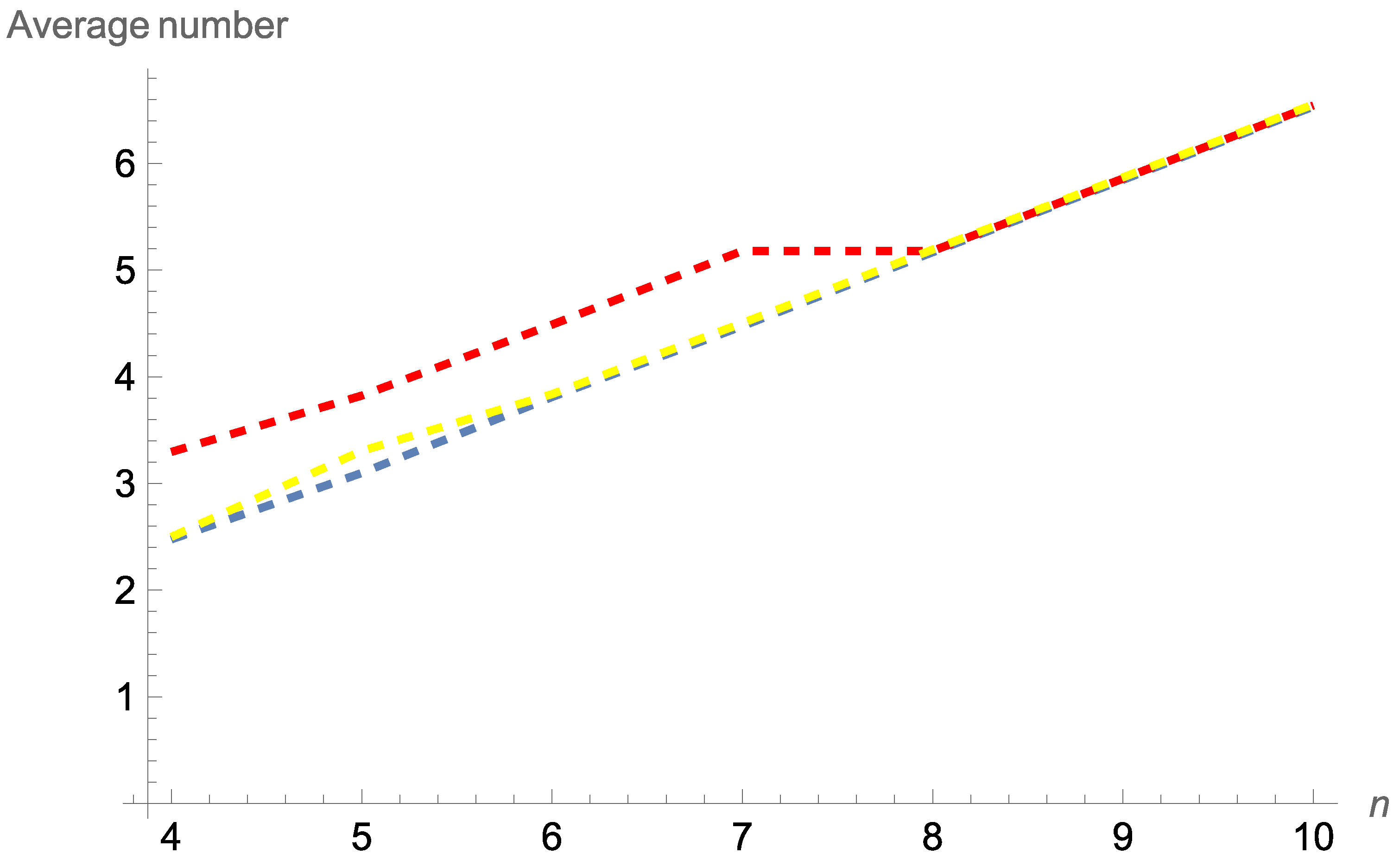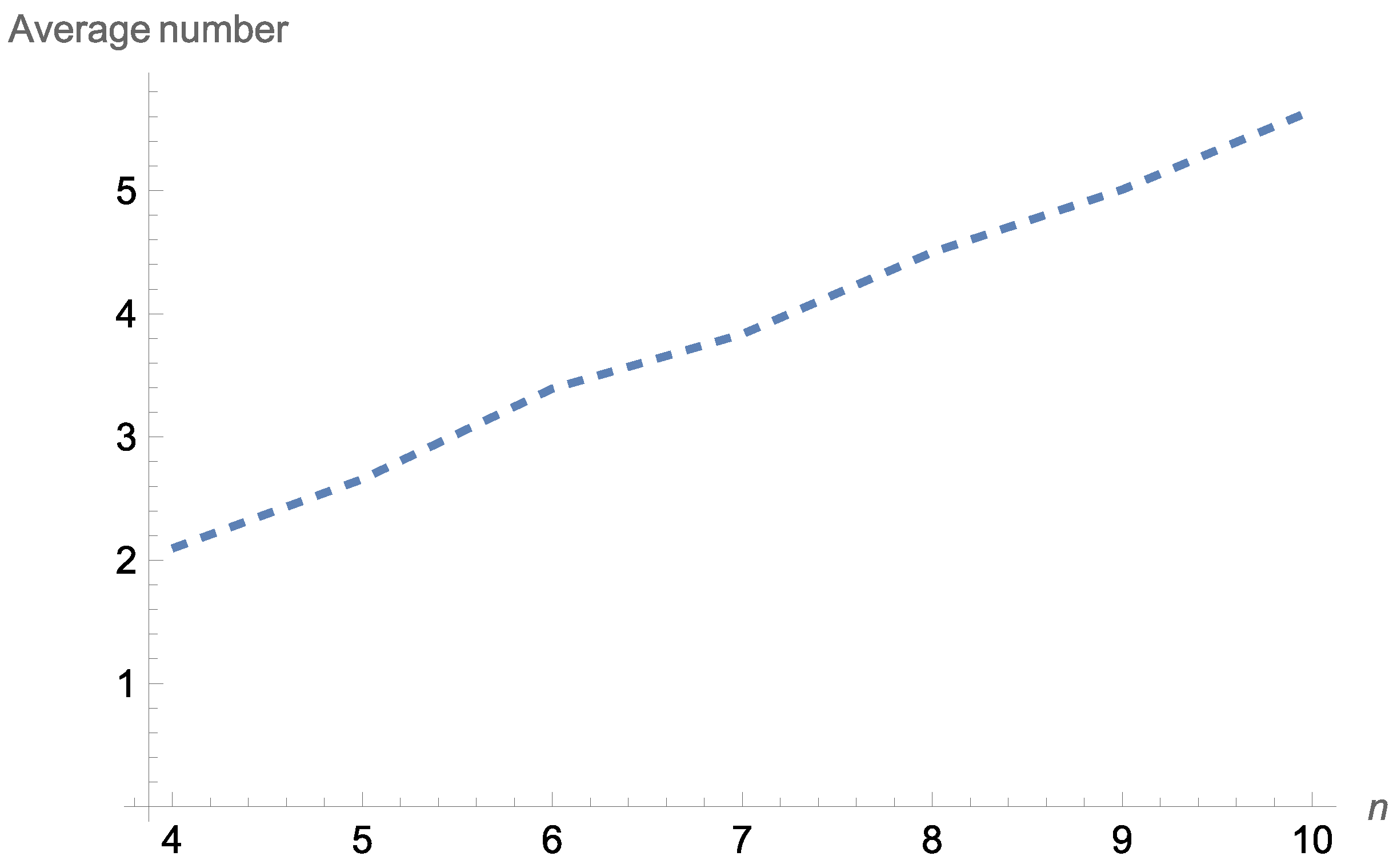Figure 1 displays the average number of working components at a given time point $t$ for a consecutive two-out-of-n system with exchangeable components under the Farlie–Gumbel–Morgenstern model.

Note that the average number of working components in all cases considered was simply computed as the mean of all possible values, which could be observed under the specific design. Figure 1 reveals that the average number of working components at a given time point $t$ for a consecutive two-out-of-n system increased as $n$ increased. In addition, it seems that among the cases considered, the choice $a=0.6 \left(red\right)$ resulted in a larger number of working components. However, when the order of the structure became large ($n>7$), the differences between the corresponding average numbers were negligible.

We next investigated the two-within k-out-of-n: F system with exchangeable components. Based on Proposition 2, we studied the random variable $\left\{N_n\left(t\right)\left|T>t\right.\right\}$ under both the Farlie–Gumbel–Morgenstern multivariate model and the Pareto multivariate model.

Looking at

Table 2. Distribution of $\left\{N_n\left(t\right)\left|T>t\right.\right\}$ for the two-within consecutive three-out-of-n system with an order of 5.

			Farlie–Gumbel–Morgenstern Distribution	Pareto Distribution
a	t	ξ	$\mathit{P}\left({\mathit{N}}_{\mathit{n}}\left(\mathit{t}\right)=\mathit{\xi }\left|\mathit{T}>\mathit{t}\right.\right)$	$\mathit{P}\left({\mathit{N}}_{\mathit{n}}\left(\mathit{t}\right)=\mathit{\xi }\left|\mathit{T}>\mathit{t}\right.\right)$
0.2	1.5	1	0.00000	0.00000
		2	0.00000	0.00000
		3	0.66999	0.01781
		4	0.31241	0.13295
		5	0.01760	0.84924
	2	1	0.00000	0.00000
		2	0.00000	0.00000
		3	0.79114	0.02515
		4	0.20262	0.15267
		5	0.00624	0.82218
	2.5	1	0.00000	0.00000
		2	0.00000	0.00000
		3	0.86968	0.02865
		4	0.12806	0.16052
		5	0.00226	0.81083
0.8	1.5	1	0.00000	0.00000
		2	0.00000	0.00000
		3	0.68313	0.07752
		4	0.30070	0.36551
		5	0.01617	0.55697
	2	1	0.00000	0.00000
		2	0.00000	0.00000
		3	0.79731	0.10404
		4	0.19682	0.39406
		5	0.00587	0.50190
	2.5	1	0.00000	0.00000
		2	0.00000	0.00000
		3	0.87227	0.11604
		4	0.12556	0.40359
		5	0.00217	0.48037

, we can readily conclude that $P\left(N_n\left(t\right)=\xi \left|T>t\right.\right)$ depended on $a,t,\xi$, but there was non-monotone relation between them under the Farlie–Gumbel–Morgenstern distribution. Note that the results appearing in Table 2 were produced under the design $\{n=5,k=3\}$ while the remaining parameters varied.

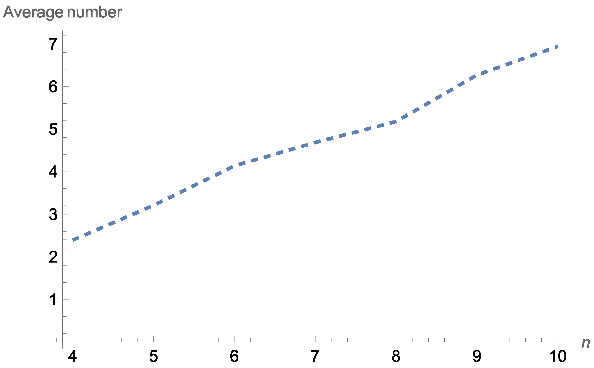
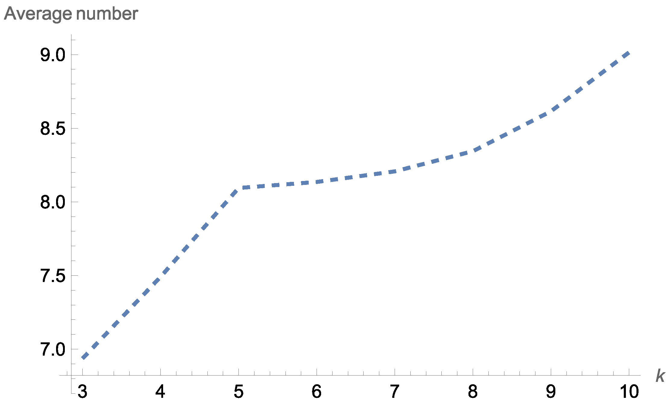
We next investigated the impact of the aforementioned parameters on the underlying distribution of the random variable $\left\{N_n\left(t\right)\left|T>t\right.\right\}$. Figure 2 and Figure 3 display the average number of working components at a given time point $t$ for the two-within consecutive k-out-of-n system with exchangeable components under the Farlie–Gumbel–Morgenstern model ($a=0.8$).

With the aid of Figure 2, it is straightforward that the average number of working components at a given time point $t$ for a two-within consecutive three-out-of-n: F system increased as $n$ increased.

For constructing Figure 3, a pre-specified design was implemented. More precisely, we considered the two-within consecutive k-out-of-ten: F system for several different values of the parameter k, while the distribution parameter $a$ was assumed to be equal to 0.8. Figure 3 reveals that the average number of working components at a given time point $t$ for a two-within consecutive k-out-of-ten: F system increased as $k$ increased.

By applying a parallel argumentation, one may readily carry out a corresponding numerical investigation for both reliability structures with two common failure criteria, which have been studied before. Firstly, we focused on the $(n,f,2)$ system consisting of exchangeable components.

Table 3. Distribution of $\left\{N_n\left(t\right)\left|T>t\right.\right\}$ for the $(n,f,2)$ system with an order of 5.

			Farlie–Gumbel–Morgenstern Distribution	Pareto Distribution
a	t	ξ	$\mathit{P}\left({\mathit{N}}_{\mathit{n}}\left(\mathit{t}\right)=\mathit{\xi }\left|\mathit{T}>\mathit{t}\right.\right)$	$\mathit{P}\left({\mathit{N}}_{\mathit{n}}\left(\mathit{t}\right)=\mathit{\xi }\left|\mathit{T}>\mathit{t}\right.\right)$
0.2	1.5	1	0.00000	0.00000
		2	0.00000	0.00000
		3	0.80239	0.03499
		4	0.18707	0.13063
		5	0.01054	0.83438
	2	1	0.00000	0.00000
		2	0.00000	0.00000
		3	0.88339	0.04907
		4	0.11312	0.14892
		5	0.00349	0.80201
	2.5	1	0.00000	0.00000
		2	0.00000	0.00000
		3	0.93030	0.05570
		4	0.06849	0.15605
		5	0.00121	0.78825
0.8	1.5	1	0.00000	0.00000
		2	0.00000	0.00000
		3	0.81174	0.14389
		4	0.17865	0.33921
		5	0.00961	0.51690
	2	1	0.00000	0.00000
		2	0.00000	0.00000
		3	0.88723	0.18848
		4	0.10951	0.35693
		5	0.00326	0.45459
	2.5	1	0.00000	0.00000
		2	0.00000	0.00000
		3	0.93178	0.20794
		4	0.06706	0.36164
		5	0.00116	0.43042

provides several probabilities which were connected to the distribution of the random variable $\left\{N_n\left(t\right)\left|T>t\right.\right\}$ for the $(n,f,2)$ system with an order of five. The results were produced under the assumption that the components of the underlying structure had either the Farlie–Gumbel–Morgenstern multivariate distribution or the corresponding Pareto one with different choices for the respective parameter.

Based on the numerical results presented in Table 3, we readily deduced that $P\left(N_n\left(t\right)=\xi \left|T>t\right.\right)$ depended on $a,t,\xi$, but there was a non-monotone relation between them under the Farlie–Gumbel–Morgenstern distribution. Since the results appearing in Table 3 shared a common value for the design parameter $n$, it seems intriguing to examine how the underlying distribution of the random variable $\left\{N_n\left(t\right)\left|T>t\right.\right\}$ is influenced by the aforementioned parameter.

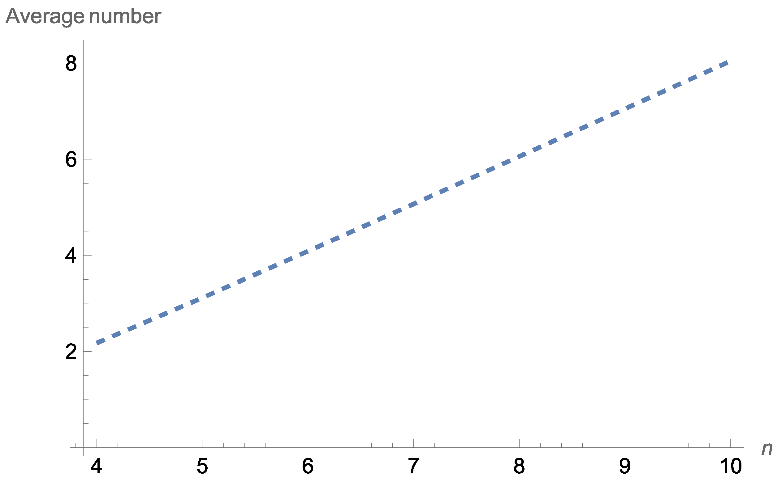
Figure 4 displays the average number of working components at a given time point $t$ for an $(n,f,2)$ system consisting of exchangeable components under the Farlie–Gumbel–Morgenstern model.

Figure 4 reveals that the average number of working components at a given time point $t$ for an $(n,f,2)$ system increased as $n$ increased.

Finally, we focus on the so-called <$n,f,2>$ system consisting of exchangeable components. Based on Proposition 4, we studied the random variable $\left\{N_n\left(t\right)\left|T>t\right.\right\}$ under both the Farlie–Gumbel–Morgenstern multivariate model and Pareto multivariate model.

Based on

Table 4. Distribution of $\left\{N_n\left(t\right)\left|T>t\right.\right\}$ for the <$n,3,2>$ system with an order of 5.

			Farlie–Gumbel–Morgenstern Distribution	Pareto Distribution
a	t	ξ	$\mathit{P}\left({\mathit{N}}_{\mathit{n}}\left(\mathit{t}\right)=\mathit{\xi }\left|\mathit{T}>\mathit{t}\right.\right)$	$\mathit{P}\left({\mathit{N}}_{\mathit{n}}\left(\mathit{t}\right)=\mathit{\xi }\left|\mathit{T}>\mathit{t}\right.\right)$
0.2	1.5	1	0.00000	0.00000
		2	0.23903	0.00287
		3	0.66300	0.05683
		4	0.09275	0.12728
		5	0.00522	0.81302
	2	1	0.00000	0.00000
		2	0.37685	0.00517
		3	0.57742	0.07878
		4	0.04437	0.14346
		5	0.00137	0.77259
	2.5	1	0.00000	0.00000
		2	0.52022	0.00649
		3	0.45914	0.08892
		4	0.02028	0.14949
		5	0.00036	0.75510
0.8	1.5	1	0.00000	0.00000
		2	0.25335	0.01477
		3	0.65544	0.21559
		4	0.08655	0.30495
		5	0.00466	0.46469
	2	1	0.00000	0.00000
		2	0.38698	0.02469
		3	0.56958	0.27217
		4	0.04218	0.30926
		5	0.00126	0.39388
	2.5	1	0.00000	0.00000
		2	0.52639	0.03005
		3	0.45368	0.29523
		4	0.01959	0.30806
		5	0.00034	0.36666

, we can conclude that $P\left(N_n\left(t\right)=\xi \left|T>t\right.\right)$ depended on $a,t,\xi$, but there was a non-monotone relation between them under the Farlie–Gumbel–Morgenstern model. Note that the results appearing in Table 4 were produced under the design where $\{n=5\}$. We next examine the influence of the aforementioned parameter on the underlying distribution of the random variable $\left\{N_n\left(t\right)\left|T>t\right.\right\}$. Figure 5 displays the average number of working components at a given time point $t$ for the <$n,3,2>$ system with exchangeable components under the Farlie–Gumbel–Morgenstern model ($a=0.8$).

With the aid of Figure 5, it is straightforward that the average number of working components at a given time point $t$ for an <$n,f,2>$ system increased as $n$ increased.

4. Discussion

In the present work, the number of working components within a consecutive-type reliability structure was examined in some detail. The theoretical results were produced under exchangeability. Different multivariate distributions were taken into account, while the main contribution of the manuscript is related to the corresponding probability mass function. Several numerical results were illustrated for different consecutive-type systems, and some conclusions regarding the influence of the respective design parameters were made. The computation procedure proved to be quite complicated due to the large number of design parameters. In fact, the selection of the most suitable values for each parameter in order to reach the desired level of performance seems to be time-consuming. In addition, it could be interesting to apply alternative distributional models which are appropriate in practical problems or investigate different reliability structures.