Article

Mass Conservative Time-Series GAN for Synthetic Extreme Flood-Event Generation: Impact on Probabilistic Forecasting Models

by
Divas Karimanzira
System Technique and Image Exploitation IOSB, Fraunhofer Institute for Optronics, Am Vogelherd 90, 98693 Ilmenau, Germany
Stats 2024, 7(3), 808-826; https://doi.org/10.3390/stats7030049
Submission received: 2 July 2024 / Revised: 26 July 2024 / Accepted: 30 July 2024 / Published: 3 August 2024

Abstract

:
The lack of data on flood events poses challenges in flood management. In this paper, we propose a novel approach to enhance flood-forecasting models by utilizing the capabilities of Generative Adversarial Networks (GANs) to generate synthetic flood events. We modified a time-series GAN by incorporating constraints related to mass conservation, energy balance, and hydraulic principles into the GAN model through appropriate regularization terms in the loss function and by using mass conservative LSTM in the generator and discriminator models. In this way, we can improve the realism and physical consistency of the generated extreme flood-event data. These constraints ensure that the synthetic flood-event data generated by the GAN adhere to fundamental hydrological principles and characteristics, enhancing the accuracy and reliability of flood-forecasting and risk-assessment applications. PCA and t-SNE are applied to provide valuable insights into the structure and distribution of the synthetic flood data, highlighting patterns, clusters, and relationships within the data. We aimed to use the generated synthetic data to supplement the original data and train probabilistic neural runoff model for forecasting multi-step ahead flood events. t-statistic was performed to compare the means of synthetic data generated by TimeGAN with the original data, and the results showed that the means of the two datasets were statistically significant at 95% level. The integration of time-series GAN-generated synthetic flood events with real data improved the robustness and accuracy of the autoencoder model, enabling more reliable predictions of extreme flood events. In the pilot study, the model trained on the augmented dataset with synthetic data from time-series GAN shows higher NSE and KGE scores of NSE = 0.838 and KGE = 0.908, compared to the NSE = 0.829 and KGE = 0.90 of the sixth hour ahead, indicating improved accuracy of 9.8% NSE in multistep-ahead predictions of extreme flood events compared to the model trained on the original data alone. The integration of synthetic training datasets in the probabilistic forecasting improves the model’s ability to achieve a reduced Prediction Interval Normalized Average Width (PINAW) for interval forecasting, yet this enhancement comes with a trade-off in the Prediction Interval Coverage Probability (PICP).

1. Introduction

Extreme flood events present significant challenges to communities worldwide, causing severe impacts on infrastructure, property, and human lives. Forecasting these events is critical for disaster preparedness and response, yet traditional models often struggle to capture their complexity and variability, leading to inaccurate predictions. The research gap in flood forecasting that we cover in this paper is simply the challenge of obtaining enough data from extreme events and consequently dealing with imbalanced data. In flood forecasting and risk assessment, two common approaches for generating synthetic data to simulate extreme flood events are through numerical or hydrological models and machine-learning techniques like Generative Adversarial Networks. Numerical or hydrological models use physical principles and domain knowledge to simulate the complex processes involved in flood events, providing physically interpretable data. On the other hand, time series-based Generative Adversarial Networks (GANs) utilize deep learning algorithms to generate synthetic data that capture the temporal dynamics and patterns present in the original dataset, offering a data-driven approach to data generation.
Numerical or hydrological models have been widely used in flood modeling and simulation due to their ability to incorporate domain knowledge and physical principles. These models simulate the behavior of rivers, rainfall–runoff processes, and other hydrological phenomena to generate synthetic flood data that can be used for forecasting and risk assessment [1]. Even though numerical models can generate unseen flood events, they have drawbacks in that they are computationally intensive and require complex calibration processes. Numerical models often involve solving a set of partial differential equations that represent the physical processes governing flood events, such as rainfall–runoff, river flow, and inundation dynamics. These computations can be time-consuming and resource-intensive, particularly for simulating large-scale or extreme flood events. Additionally, numerical models require extensive calibration and validation to ensure their accuracy and reliability in generating synthetic flood data [2]. The model parameters and equations need to be calibrated using observed data, which can be challenging due to uncertainties in the input data, model structure, and boundary conditions. The calibration process may involve iterative adjustments and sensitivity analyses, further adding to the complexity and computational burden of using numerical models for synthetic data generation. Moreover, numerical models may have limitations in capturing the full range of variability and complexity of flood events, especially in extreme or rare scenarios. The simplifications and assumptions made in the model equations and parameterizations can lead to biases and inaccuracies in the synthetic flood data generated, affecting the reliability of flood-forecasting and risk-assessment applications.
In contrast, the state-of-the-art Generative Adversarial Network (GAN) models learn the underlying data distribution from the input dataset and generates synthetic data that captures the temporal dependencies and patterns present in the original data [3]. In recent years, Generative Adversarial Networks (GANs) have emerged as a promising tool for generating synthetic time-series data, including flood events. There are several Generative Adversarial Networks (GANs) that can be suitable for generating flood-event time-series data, each with its own strengths and applications. For example, SINGAN (Spatiotemporal Interactive Generative Adversarial Networks) is a GAN architecture designed for generating spatiotemporal data, such as time-series data with spatial dependencies. SINGAN incorporates both spatial and temporal convolutional layers in its generator and discriminator networks to capture the complex interactions between spatial and temporal dimensions. SINGAN has been applied in generating synthetic weather data and climate simulations [4]. The TSGAN (Time-Series Generative Adversarial Network) is a GAN variant specifically designed for generating synthetic time-series data with temporal dependencies and patterns [5]. TSGAN incorporates recurrent neural networks (RNNs) in its generator and discriminator networks to capture the sequential nature of time-series data and generate realistic and coherent sequences. TSGAN has been applied in various time-series data-generation tasks, including financial data modeling, energy forecasting, and environmental data simulation. FloodGAN was used in [6] to generate Synthetic High-Resolution Radar Rainfall Data using Generative Adversarial Networks. Specifically, TimeGAN [7,8] and RTSGAN [9] offer a unique advantage for flood-forecasting applications due to its ability to generate synthetic time-series data that closely mimic the characteristics of real flood events. By training TimeGAN or RTSGAN on historical flood data, researchers can generate a diverse set of synthetic flood scenarios that capture the variability and complexity of extreme events. These synthetic data can be used to augment existing flood-forecasting models, enhance their predictive capabilities, and improve resilience to extreme flood events. Additionally, TimeGAN can help address data scarcity issues in regions with limited historical flood data, enabling more robust and accurate flood forecasting in vulnerable areas [7].
Successful time-series modeling requires capturing not only the features’ distributions within each time point but also the dynamics of these features over time. Studies like “FloodGAN” by [6] demonstrate how GANs can generate synthetic data to enhance flood-forecasting models. Research by [8] explored TimeGAN’s application in generating synthetic flood data to improve forecasting models, while [10] investigated its impact on enhancing predictions in the Yangtze River Basin. Additionally, a review by [11] provides insights into GANs’ applications for generating synthetic time-series data in flood forecasting and extreme event modeling. The study in [12] shows the superiority of the RTSGAN over TimeGAN in terms of model stability, reliability, and accuracy.
In this paper, we advance the state of the art in flood forecasting by leveraging time series-based GANs to generate synthetic extreme flood events. Our contribution lies in the modification and application of TimeGAN, a cutting-edge Generative Adversarial Network, to generate realistic synthetic flood data that captures the temporal dependencies and complexities of real flood events. The novelty of the paper includes the incorporation of constraints related to mass conservation, energy balance, and hydraulic principles into the TimeGAN model through appropriate regularization terms in the loss function to improve the realism and physical consistency of the generated extreme flood-event data. These constraints ensure that the synthetic flood-event data generated by the Mass Conservative Time-Series GAN (MC-TSGAN) adhere to fundamental hydrological principles and characteristics, enhancing the accuracy and reliability of flood-forecasting and risk-assessment applications. We also applied space-filling sampling [13] with validation to reduce the introduction of large biases and to improve the data quality. This approach represents a significant advancement in the field of flood forecasting, as it addresses the limitations of traditional models in capturing the variability and dynamics of extreme flood events. The performance of the developed models will be tested based on a case study, where we will evaluate the accuracy and reliability of the MC-TSGAN-generated synthetic flood data in enhancing flood-forecasting models. This case study provides valuable insights into the practical application of our approach and its impact on predicting and mitigating the impacts of extreme flood events.
The rest of the paper delves into the detailed description of the methodology used in the study, including the implementation of the Mass Conservative Time-Series Generative Adversarial Network (MC-TSGAN) model in Section 2. An overview of the materials and datasets utilized in the research is given. The experimental setup, including data preprocessing, model training, and validation procedures, are explained, and the description of the execution process for generating synthetic flood data and evaluating the performance of the MC-TSGAN model is given in Section 2.3. In Section 3, the results obtained from the experiments, including the accuracy and reliability of the synthetic flood data generated by MC-TSGAN and the analysis of the model’s performance metrics and comparison with baseline models, are presented. In-depth discussions on the findings and implications of the study, the identification of limitations in the methods used and potential areas for improvement, and the exploration of future research directions and perspectives for enhancing flood-forecasting capabilities are the focus of Section 4. In Section 5, a summary of the key findings and outcomes of the study, including concluding remarks on the effectiveness of using MC-TSGAN for generating synthetic flood data and its impact on flood-forecasting models will be given.

2. Materials and Methods

2.1. Case Study

The study focused on the Ahrtal region in Germany, an area known for its scenic beauty and cultural significance. The region experienced severe flooding, which prompted the selection of three gauge stations as key monitoring points to assess the impact of the floods. These gauge stations were strategically located within the Ahrtal region to collect data on water levels, flow rates, and other hydrological parameters during the flood events. The data from the study area for the flood-forecasting application include various types of information crucial for understanding and predicting flood events. These data encompass historical precipitation data, forecast precipitation data from the ECMWF (European Centre for Medium-Range Weather Forecasts), soil-type information, and water-level measurements recorded at a resolution of 10–15 min. Historical precipitation data provide records of past rainfall events, offering insights into the amount, intensity, and distribution of rainfall in the region. Forecast precipitation data from the ECMWF deliver predictions of future rainfall events, aiding in anticipating upcoming rainfall patterns and intensities for early warning and preparation. Soil-type information categorizes the various soil types based on properties like texture, permeability, and water-holding capacity, essential for evaluating soil infiltration capacity and runoff generation during heavy rainfall. Water-level measurements record water levels in rivers, streams, or water bodies, providing real-time data on hydrological conditions for monitoring changes and assessing flood-event magnitudes. This comprehensive dataset aids in analyzing flood dynamics, enhancing flood-forecasting accuracy, and supporting effective decision-making in flood risk management and disaster preparedness.

2.2. Methods

2.2.1. Methodological Approach

The methodology for leveraging GANs to generate synthetic extreme flood events for flood-forecasting applications involves a series of steps designed to enhance the accuracy and reliability of flood-forecasting models. The comprehensive methodology encompasses data collection, MC-TSGAN training and evaluation, data augmentation, forecast model training, and evaluation for multistep-ahead predictions. Here is a detailed description of each step:
  • Data Collection and Spatial Data Integration
The first step involves collecting historical flood data from multiple monitoring sites, including river flow rates, precipitation levels, and water levels. These data are essential for training the MC-TSGAN model and generating synthetic flood events that closely resemble real flood data. Additionally, spatial and temporal data from various locations are gathered to capture the spatial variability and dependencies across different sites. Data collected from multiple sites are integrated into a unified dataset that captures the spatial variability and relationships between different locations. This accounts for spatial dependencies by considering the interactions and correlations between data points from different sites when training the MC-TSGAN model. Before generating synthetic flood data using the MC-TSGAN model, it is essential to preprocess the flood time-series data to ensure optimal performance and accuracy in the data-generation process. The preprocessing steps involve normalization and segmentation of the flood time-series data to create a structured input format for the MC-TSGAN model. Normalizing the data ensures that all features have a similar range and distribution, preventing certain variables from dominating the learning process. The segmentation process involves dividing the flood time-series data into sequential segments or windows to create a three-dimensional (3D) dataset. Each segment represents a subset of the flood sequence, capturing the temporal dependencies and patterns within the data.
2.
MC-TSGAN Training
The historical flood data collected in the previous step are used to train the MC-TSGAN model. MC-TSGAN is specifically designed to capture the temporal dependencies and relationships within time-series data. The model learns the patterns and distributions present in the historical flood data, allowing it to generate synthetic flood events that exhibit similar characteristics and dynamics to real flood events.
3.
Data Augmentation
The MC-TSGAN-generated synthetic flood events are combined with the original historical flood data to create an augmented dataset. This augmented dataset contains a mix of real and synthetic data, providing a broader range of flood scenarios for training the forecasting models. The integration of synthetic data enhances the dataset’s variability and complexity, improving the model’s ability to predict extreme flood events accurately.
4.
Flood forecast model training
A forecasting model based on the encoder–decoder technique and a Long Short-Term Memory (LSTM) network is selected for predicting flood events based on the augmented dataset. The model is trained on the combined dataset to capture the spatial and temporal patterns in the data and improve the accuracy of flood-event predictions. The training process allows the model to learn from both real and synthetic data, enhancing its predictive capabilities.
5.
Evaluation
The evaluation is composed of two parts, (1) evaluation of the generation process (i.e., MC-TSGAN) and (2) the evaluation of the forecasting model based on augmented data. The generation of the synthetic data was performed using principal component analysis (PCA), t-SNE (t-Distributed Stochastic Neighbor Embedding), and t-statistics.

2.2.2. Structure and Training of the MC-TSGAN

As illustrated in [3], a Time-Series Generative Adversarial Network consists of several key components that work together to generate synthetic time-series data with temporal dependencies, as shown in Figure 1. The structure of time-series GAN typically includes a generator, a discriminator, and an embedding network, each serving a specific function in the model.
Our development is based on both TimeGAN and RTSGAN. The generator is responsible for generating synthetic time-series data that closely resemble real data. It typically consists of recurrent neural network (RNN) layers, such as LSTM (Long Short-Term Memory) or GRU (Gated Recurrent Unit), to capture the temporal dependencies in the data. The generator takes random noise vectors as input and generates sequences of data points that mimic the patterns and characteristics of the real time-series data. In our case, the generation module incorporates a Wasserstein Generative Adversarial Network (WGAN) to generate new data points in the same latent space learned by the embedding network. WGAN is a type of GAN that focuses on improving the training stability and convergence of the generator network. By training the WGAN to generate vectors in the latent space defined by the embedding network, MC-TSGAN can create new data points that exhibit similar characteristics to the original time-series data. This process allows MC-TSGAN to generate realistic time-series data that respect the original feature distributions and temporal dynamics of the input data.
The discriminator in MC-TSGAN is a binary classifier that distinguishes between real and synthetic time-series data. It helps guide the generator to produce more realistic synthetic data by providing feedback on the quality of the generated samples. The discriminator is typically implemented using convolutional neural network (CNN) layers to process the time-series data and classify them as real or synthetic.
The embedding network in MC-TSGAN is used to learn a low-dimensional representation of the time-series data that captures the latent features and temporal dependencies present in the data. It helps improve the generation of synthetic data by providing a compact representation of the data. The embedding network is often implemented using autoencoder architectures, such as variational autoencoders (VAEs) or denoising autoencoders, to learn a meaningful representation of the time-series data and extract relevant features for generating synthetic data.
We modified the TimeGAN to MC-TSGAN model to improve the generation of extreme flood events by incorporating domain-specific knowledge and constraints related to flood events into the TimeGAN architecture. The Theory-Guided Data Science (TGDS) introduces a novel approach to integrating physical constraints into deep learning (DL) models, ensuring that their predictions align with physical principles [14,15,16,17]. We introduced domain-specific constraints and knowledge into the TimeGAN architecture to ensure that the generated synthetic data align with the physical laws and characteristics of flood events. We incorporated constraints related to mass conservation, energy balance, and hydraulic principles to improve the realism of the generated flood-event data. Incorporating constraints related to mass conservation, energy balance, and hydraulic principles into the MC-TSGAN model for generating extreme flood events involves modifying the loss functions and regularization terms to enforce these constraints during training.
The mass conservation principle states that the total mass of water entering a system must equal the total mass of water leaving the system. This can be enforced in two ways, (1) by incorporating the mass conservation constraint into the architecture of the LSTM network or (2) by adding a regularization term to the loss function that penalizes deviations from mass conservation principles. For the first method, the LSTMs in the generator and discriminator were modified, as shown by Equations (7)–(13). Input variables are categorized into mass inputs ( x t ) and auxiliary inputs ( a t ). For mass inputs, normalized activation functions are applied in the input gate ( i t ) and forget gate ( R t ) to ensure mass conservation between the mass inputs and the previous cell state ( c t 1 ). Additionally, the output gate ( o t ) subtracts the output mass ( h t ) from the total mass ( m t ) to maintain mass conservation between the cell state ( c t ) and the output mass.
i t = σ ~ W i a t + U i c t 1 c t 1 1 + V i x t + b i
o t = σ W o a t + U o c t 1 c t 1 1 + V o x t + b o
R t = R e L u ~ W r a t + U r c t 1 c t 1 1 + V r x t + b r
m t = R t c t 1 + i t x t
c t = 1 o t m t
h t = o t m t
y t = i = 2 n h i t
where W, U, and V represent learnable weights; b denotes the learnable bias parameters; and σ ~   and R e L u ~ indicate the normalized sigmoid function and the normalized function, respectively.
In the second method, this can be enforced as a constraint during the generation of synthetic flood-event data by adding a regularization term to the loss function that penalizes deviations from mass conservation principles. The regularization term was formulated as follows:
L o s s Q = λ Q t Q i n t Q o u t
where t Q i n represents the input water mass at time step, t; t Q o u t represents the output water mass at time step, t; and λ Q is a regularization parameter that controls the importance of the mass conservation constraint.
The energy-balance principle ensures that the energy input into a system equals the energy output, considering factors such as potential energy, kinetic energy, and losses due to friction and turbulence to incorporate energy terms as time-series data into the MC-TSGAN model for generating extreme flood events, energy-related variables, or parameters from relevant sources. Meteorological stations provide time-series data on weather variables such as temperature, humidity, wind speed, and solar radiation. These weather variables were used to calculate energy-related parameters, such as potential evapotranspiration, and hydrological monitoring stations offer time-series data on river flow rates, water levels, and precipitation. These hydrological variables were used to estimate hydraulic energy potential, such as the kinetic energy of flowing water and potential energy from water levels. Like mass conservation, the energy-balance constraint is incorporated into the TimeGAN model through a regularization term in the loss function. The regularization term for energy balance can be formulated as follows:
L o s s E = λ E t E i n t E o u t
where t E i n represents the input energy input at time step, t; t E o u t represents the energy output at time step, t; and λ E is a regularization parameter for the energy-balance constraint.
Hydraulic principles govern the flow of water in rivers and channels, including factors such as flow velocity, channel geometry, and frictional losses. These principles can be incorporated into the MC-TSGAN model to ensure that the generated flood-event data adhere to hydraulic constraints. To enforce hydraulic principles, additional constraints related to flow continuity, Manning’s equation, or channel capacity were included in the loss function or as regularization terms. Manning’s equation relates flow velocity, channel geometry, and roughness coefficient in open-channel flow, providing insights into the relationship between flow characteristics and channel properties. We can incorporate Manning’s equation constraint by including terms that enforce the relationship between flow velocity, channel slope, and roughness coefficient in the loss function. This can help ensure that the synthetic flood-event data generated by MC-TSGAN adhere to the principles of open-channel flow. By incorporating these constraints related to mass conservation, energy balance, and hydraulic principles into the MC-TSGAN model through appropriate regularization terms in the loss function, we can improve the realism and physical consistency of the generated extreme flood-event data. These constraints ensure that the synthetic flood-event data generated by MC-TSGAN adhere to fundamental hydrological principles and characteristics, enhancing the accuracy and reliability of flood-forecasting and risk-assessment applications.
The MC-TSGAN is trained using a combination of adversarial-training and unsupervised-learning techniques. The generator and discriminator are trained in an adversarial manner, where the generator aims to fool the discriminator by generating realistic synthetic data, while the discriminator aims to distinguish between real and synthetic data accurately. The embedding network is trained simultaneously with the generator and discriminator to learn a compact representation of the data that can be used to generate high-quality synthetic time-series data in order to train the MC-TSGAN model specifically to generate extreme flood events by focusing on capturing the tail distributions and rare events in the data. This can be achieved by adjusting the loss functions, regularization techniques, or sampling strategies to emphasize the generation of extreme values in the synthetic flood data. Space-filling sampling was applied to reduce statistical errors. Space-filling sampling is a technique used to evenly distribute sample points throughout a given space to reduce statistical errors and improve the accuracy of data analysis [13]. In the context of the MC-TSGAN, we applied space-filling sampling by selecting a set of representative data points from the time-series dataset that were evenly spaced out in time. We first divided the time-series data into equal intervals and then selected a subset of data points from each interval. This subset of data points was chosen in such a way that they were evenly distributed across the entire time series, ensuring that the data points were representative of the entire dataset. By using space-filling sampling in this way, we were able to reduce the statistical errors in the time-series GAN by ensuring that the generated data points were more accurate and representative of the underlying distribution of the time-series dataset. This helped to improve the overall performance and reliability of the MC-TSGAN model. During the training process, the modified MC-TSGAN model learns to generate synthetic flood-event data by balancing the objectives of capturing temporal dependencies, adhering to physical constraints, and maximizing realism. The model iteratively adjusts the generator and discriminator networks based on the feedback provided by the discriminator and the constraints enforced through the augmented loss functions. By incorporating domain-specific knowledge and constraints into the training process, the MC-TSGAN model can generate extreme flood-event data that are both realistic and consistent with the physical principles governing flood events.

2.2.3. Probabilistic Flood-Forecasting Model

In this paper, the probabilistic flood-forecasting model serves only to evaluate the impact of the generated synthetic data on its performance. Therefore, it is discussed only briefly. We refer the reader to our previous paper [18] for a detailed description. The flood-forecasting model is based on encoder–decoder principles; it is designed to handle the data of different timescales and incorporates various input parameters to predict future flood events, as shown in Figure 2.
The model takes historical flood events, rainfall data, soil moisture levels, catchment characteristics, and future rainfall forecast data as inputs to generate probabilistic flood forecasts. The model structure includes an encoder component that processes the historical and constant input data and extracts relevant features, followed by a decoder component that generates predictions based on the encoded information and the future forecasted information about the precipitation. The following are its key features:
  • Input data: The model integrates a diverse range of input data, including historical flood events, rainfall measurements, soil moisture levels, catchment characteristics, and future rainfall forecasts. This comprehensive dataset enables the model to capture the complex interactions and dynamics influencing flood events.
  • Time-series handling: The model is capable of handling the time-series data of varying timescales, allowing it to analyze historical trends, short-term fluctuations, and long-term patterns in the input variables. By considering data from different time intervals, the model can provide accurate and comprehensive flood forecasts.
  • Probabilistic forecasting based on tensorflow_probability [19]: The model is modified with a probabilistic head that utilizes negative likelihood loss for training. This probabilistic approach enables the model to generate probabilistic forecasts, providing not only point estimates but also uncertainty quantification in the predictions. This is essential for assessing the reliability and confidence of the forecasted outcomes.
  • LSTM or GRU architecture: The model structure incorporates Long Short-Term Memory (LSTM) or Gated Recurrent Unit (GRU) networks, which are specialized recurrent neural network architectures well-suited for processing sequential data like time series. These architectures enable the model to capture temporal dependencies, learn from past observations, and make predictions based on sequential patterns in the input data.

2.2.4. Evaluations of MC-TSGAN Based on PCA and t-SNE

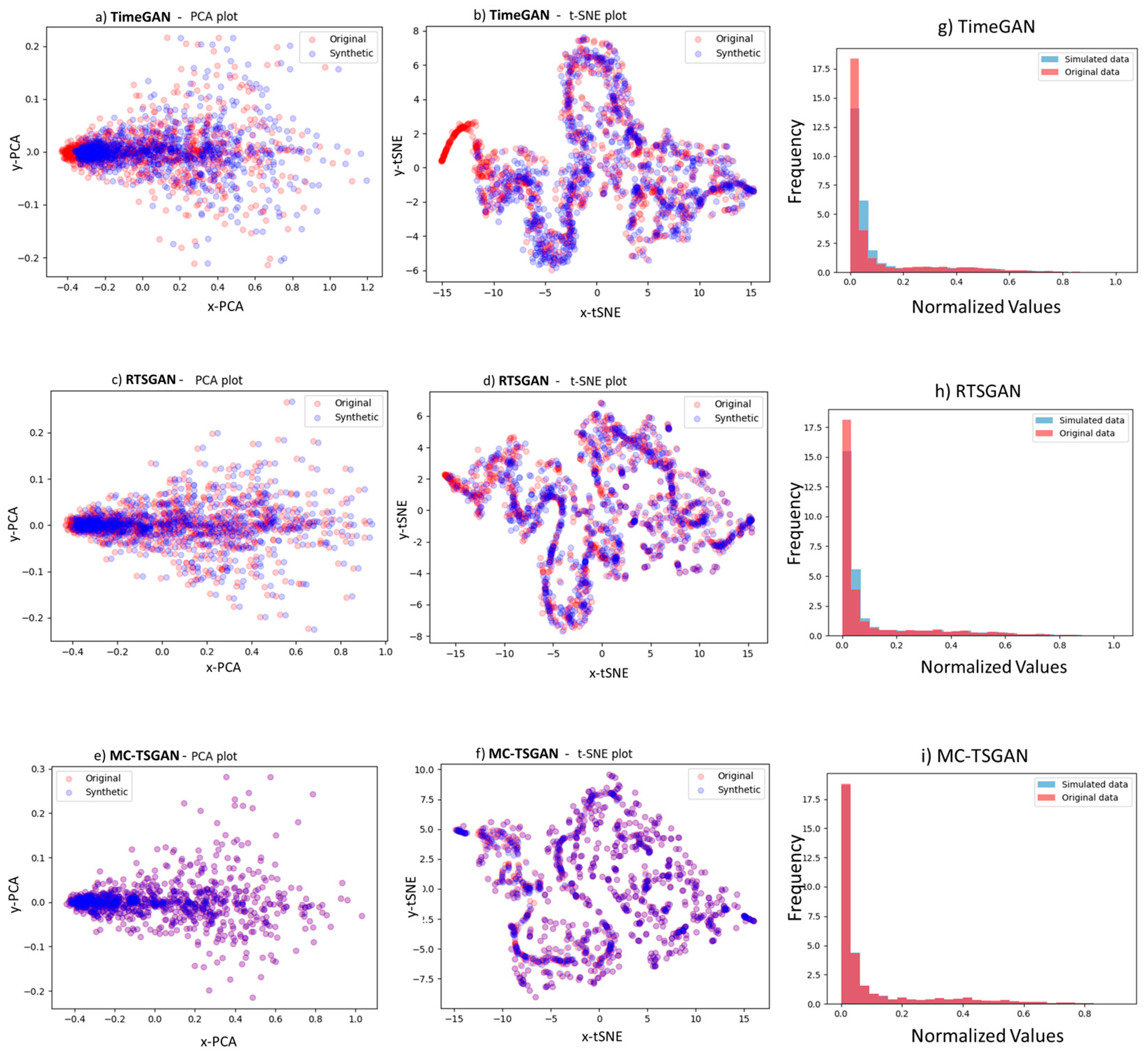
PCA (principal component analysis) and t-SNE can provide valuable insights into the generated synthetic data and help understand the underlying patterns and relationships within the data. Each of these techniques offers different perspectives on the data, and combining them can offer a comprehensive view of the data distribution. The PCA is conducted on the combined dataset of real and synthetic flood events to reduce the dimensionality of the data, and the principal components to identify the most significant features and understand the variance explained by each component are visualized by plotting the data points in the reduced-dimensional space to explore the clustering and distribution of the real and synthetic flood events. The PCA can help filter out noise and irrelevant information in the data, focusing on the most relevant features and patterns. Furthermore, t-SNE is applied to the combined dataset to visualize the high-dimensional data in a lower-dimensional space while preserving the local structure of the data. By plotting the data points in the t-SNE space to reveal clusters, patterns, and relationships between the real and synthetic flood events, t-SNE can be used to identify similarities and differences between the real and synthetic data points, highlighting any discrepancies in the data distribution.

2.2.5. Evaluation of MC-TSGAN Based on t-Statistics

The t-statistic test was conducted to compare the means of synthetic data generated by MC-TSGAN with the original data in a statistical analysis. To calculate the t-statistic for the generated data by the MC-TSGAN, we first defined a null hypothesis and an alternative hypothesis. Our null hypothesis is that the mean of the generated data is equal to the mean of the original time-series data, and the alternative hypothesis is that the means are not equal. Next, we calculate the t-statistic using the following:
t = ( x ¯ g e n x ¯ o r i g )   /   ( x σ   /   n )
where x ¯ g e n is the mean of the generated data, x ¯ o r i g is the mean of the original time-series data, x σ is the standard deviation of the generated data, and n is the number of data points in the generated data.
Once we have calculated the t-statistic, we can determine its statistical significance by comparing it to a critical value from the t-distribution with degrees of freedom equal to n − 1. If the absolute value of the t-statistic is greater than the critical value, we can reject the null hypothesis and conclude that the difference between the means of the generated data and the original data is statistically significant.

2.2.6. Evaluation of the Flood-Forecasting Model

The performance of the forecasting model is evaluated using Nash–Sutcliffe Efficiency (NSE) and Kling–Gupta Efficiency (KGE) metrics. The evaluation results provide insights into the effectiveness of using MC-TSGAN-generated synthetic data in improving flood-forecasting models and predicting extreme flood events. The model’s predictions are compared against observed flood events to assess the accuracy and reliability of the forecasts, as given by Equations (2) and (3). The Nash–Sutcliffe Efficiency (NSE) metric measures the relative magnitude of the residual variance compared to the measured data variance, with a value of 1 indicating a perfect match between model predictions and observed data. NSE is a widely used metric to evaluate the accuracy of hydrological model. On the other hand, the Kling–Gupta Efficiency (KGE) metric provides a comprehensive assessment of the model’s performance by considering correlation, bias, and variability in the predictions. A higher NSE or KGE value signifies a better agreement between the model predictions and observed data, indicating the model’s effectiveness in forecasting flood events.
N S E = 1 ( Q o b s Q s i m 2 Q o b s Q ¯ o b s 2 )
K G E = 1 r 1 2 + β 1 2 + γ 1 2 ,
where r is the correlation coefficient, β is the ratio of the standard deviation of the simulated data to the observed data, and γ is the ratio of the mean of the simulated data to the observed data.
Both the NSE and KGE provide valuable insights into the model’s ability to capture the observed rainfall–runoff relationship. However, it is important to note that these metrics have their limitations and should be interpreted in conjunction with domain knowledge.
Three metrics were collectively used to provide a comprehensive assessment of both the accuracy and reliability of the probabilistic prediction models. The Continuous Ranked Probability Score (CRPS) generalizes the MAE (Mean Absolute Error) to the case of probabilistic forecasts by comparing the cumulative distribution function of the forecast with that of the observed values. It provides a measure of the forecast’s calibration and sharpness, with lower CRPS values indicating better performance.
C R P S = 1 199 N m = 1 N n = 99 99 P y n H ( n Y m ) 2
where P is the predicted distribution, N is the number of samples in the test set, Y is the cumulative distribution function of the observed value for point m, and H(x) is the Heaviside step function (H(x) = 1 for x ≥ 0 and zero otherwise).
The Mean Prediction Interval Width (MPIW) calculates the average width of the prediction intervals. As expressed in Equation (5), it provides insight into the spread or uncertainty of the forecasted intervals, with narrower intervals indicating more precise predictions.
M P I W = 1 n i = 1 n P I i u P I i l
where n is the size of the test set, and P I i u and P I i l denote the upper and lower bounds of the 95% prediction interval, respectively.
Lastly, the Prediction Interval Coverage Probability (PICP) given by Equation (6) evaluates the coverage accuracy of prediction intervals. It measures the proportion of observed values that fall within the forecasted prediction intervals. Ideally, the coverage probability should match the specified confidence level of the prediction intervals.
P I C P = 1 n i = 1 n C ,   w h e r e   C = 1 P I i u > y i > P I i l 0 o t h e r w i s e

2.3. Experimental Setup and Simulation

The hyperparameters of the MC-TSGAN model were optimized using Bayesian optimization [20] to determine specific values for key parameters. The number of time steps was set to 24 to represent hourly data, while the latent dimension was defined as 100 to capture the underlying features of the flood data. The model architecture consisted of three layers for the generator and two layers for the discriminator to effectively learn the temporal dependencies in the data. A learning rate of 0.0002 and a batch size of 64 were selected to optimize the training process, with 1000 epochs set for model convergence. Additionally, a gradient penalty coefficient of 10 and L2 regularization with a weight of 0.001 were applied to enhance the model’s stability and generalization capabilities. These hyperparameter values were carefully chosen to maximize the MC-TSGAN model’s accuracy and performance in generating synthetic flood data for improved flood-prediction tasks.
The MC-TSGAN model was trained with spatial data, incorporating information from multiple monitoring sites to capture spatial dependencies and variability across different locations. The model was specifically tailored to generate synthetic flood events that reflect the spatial dynamics present in the data. Following training, the performance of the MC-TSGAN model was evaluated and visualized using t-statistics, principal component analysis (PCA), and t-Distributed Stochastic Neighbor Embedding (t-SNE) plots.
The PCA plots provided insights into the high-dimensional structure of the synthetic flood events, revealing the principal components that explain the variance in the data. Clusters, patterns, and relationships within the synthetic flood data were visualized based on the principal components, offering a deeper understanding of the spatial patterns present in the data. Similarly, the t-SNE plots illustrated the spatial distribution of the synthetic flood events in a lower-dimensional space while preserving the local structure of the data. Clusters and similarities between flood events were identified, revealing spatial patterns and relationships that may impact flood-forecasting accuracy. By visualizing the performance results of the TimeGAN model using PCA and t-SNE plots, valuable insights were gained into the spatial characteristics and patterns of the synthetic flood data. These visualizations provided a comprehensive view of the spatial dynamics captured by the TimeGAN model, enhancing the understanding of spatial dependencies and variability in flood events across different locations.
The original time-series data were augmented by combining the MC-TSGAN-generated synthetic flood events with the real data collected from multiple sites to create an augmented dataset for training flood-forecasting models. A forecasting model [19] leveraging the spatial and temporal information in the augmented dataset to predict extreme flood events accurately was developed and trained on both the original and augmented datasets to capture the spatial and temporal patterns in the data and enhance the accuracy of flood-event predictions.
Simulation experiments were conducted to compare the performance of flood-forecasting models trained on original data versus models trained on original data augmented with synthetically generated data from MC-TSGAN. The simulations involved generating synthetic extreme flood events using MC-TSGAN, integrating them with real flood data, training forecasting models, and evaluating their performance. The Nash–Sutcliffe Efficiency (NSE) and Kling–Gupta Efficiency (KGE) metrics were used to assess the accuracy of multistep-ahead predictions of extreme flood events. Higher NSE and KGE scores indicate better model performance in capturing the variability and dynamics of extreme flood events. By comparing the NSE and KGE scores of the model trained on the augmented dataset with synthetic data from MC-TSGAN to the model trained on the original data alone, the improvement in the forecasting model’s ability to predict extreme flood events accurately can be quantitatively assessed.
In the final experiments and ablation tests, the performance of the MC-TSGAN in generating flood events and enhancing flood-forecasting models was evaluated in comparison to the TimeGAN and RTSGAN models. The evaluation aimed to assess the effectiveness and reliability of the MC-TSGAN model in generating synthetic flood data and improving flood-forecasting capabilities.
The prediction models were developed in Python 3.6.9 with the Keras [21], TensorFlow [22], and PyTorch [23] libraries.

3. Results

Communicating flood-forecast results to the public in the form of water levels is often preferred over discharge because water levels are more easily understood and relatable to individuals in flood-prone areas [24]. Water levels directly indicate the depth of flooding in a particular location, providing a clear and intuitive representation of the potential impact of a flood event. In contrast, discharge values may be more technical and abstract, making it challenging for the public to interpret and visualize the actual extent of flooding. Therefore, the discharge predictions were converted to water levels in our results discussion.
A t-statistic of −1.67 was calculated using Equation (1) for the MC-TSGAN generated data. Next, we compare this t-statistic to the critical value from the t-distribution with n − 1 degrees of freedom for a two-tailed test at a 95% confidence level. The critical value is approximately ±1.98. Since our calculated t-statistic of −1.67 is less than the critical value of −1.98, we failed to reject the null hypothesis. This means that the difference between the means of the generated data and the original data is not statistically significant at the 0.05 level. Furthermore, the average (best) discriminative and predictive scores of MC-TSGAN on the case study were 0.0490 (0.019) and 0.0519 (0.047), respectively, as shown in Table 1.
As in [3], we conducted PCA [25] and t-SNE [26] analyses on normalized feature matrixes, and the first two principal components were selected to minimize feature dimensionality. The visualization of the performance results using a PCA plot (Figure 3e) and t-SNE (Figure 3f) shows that the synthetic flood events generated by MC-TSGAN exhibit distinct spatial patterns and clusters. In the PCA plot, the principal components reveal the underlying structure of the synthetic flood data, highlighting key features and trends in the spatial distribution of the events. Clusters and groupings of data points based on the principal components indicate similarities and relationships between different flood events, providing insights into the spatial dynamics captured by the MC-TSGAN model. Similarly, the t-SNE plot visualizes the spatial distribution of the synthetic flood events in a lower-dimensional space, preserving the local structure of the data. Clusters and patterns in the t-SNE plot further elucidate the spatial relationships and similarities among flood events, offering a detailed view of the spatial variability present in the synthetic data. The t-SNE visualization enhances the understanding of spatial dependencies and interactions between data points from different locations, providing a comprehensive representation of the spatial dynamics captured by the MC-TSGAN model.
The histogram in Figure 3i and PCA and t-SNE results (Figure 3e) demonstrate a high level of alignment and similarity between the synthetic and real flood data points, indicating a strong performance of the MC-TSGAN model in generating synthetic flood events that closely resemble the characteristics of real flood events. The almost-perfect overlap observed in the visualization of the synthetic and real data points suggests that the synthetic data generated by MC-TSGAN capture the spatial and temporal patterns present in the real flood data accurately. The close alignment between the synthetic and real data points in the PCA and t-SNE plots signifies the model’s ability to replicate the complex dynamics and dependencies of flood events, showcasing the effectiveness of MC-TSGAN in generating realistic synthetic flood data. The results indicate that the synthetic data not only capture the spatial variability and relationships within the data but also mirror the underlying patterns and structures observed in the real flood events.
Moreover, the increased diversity of the synthetic sequences, as indicated by the lower discriminative score of 0.0490 (0.0185), signifies that Time-Series GAN can produce a wider range of outputs that exhibit variability and richness. This diversity is a desirable trait in generative models, as it allows for the generation of novel and distinct sequences that capture the complexity and nuances present in the original data.
The findings from the 2D t-SNE and PCA visualizations, along with the lower discriminative score, collectively demonstrate the capability of MC-TSGAN to generate synthetic sequences that not only closely match the original data distribution but also exhibit enhanced diversity, making it a promising tool for generating realistic and varied sequences in a synthetic manner. Further tests based on spatial and temporal correlation show that when comparing the generated samples from MC-TSGAN to the original datasets, it is observed that MC-TSGAN achieves temporal correlation coefficients that are closer to those of the original data. This suggests that MC-TSGAN can better preserve the temporal correlation structure of the flood time series across different intervals, indicating its superior performance in capturing the complex spatial–temporal relationships present in the data.
The discriminative and predictive scores in Table 1 and the comparison of the Figure 3a–f, showing the results of the different GANs, TimeGAN, RTSGAN, and MC-TSGAN, show that all the methods can generate reasonable synthetic time series. Figure 4 illustrates the results of flood water prediction for the 6th hour ahead, generated by two flood-forecast models. One model was trained solely on the original data, while the other model was trained on the original data augmented with data generated by the MC-TSGAN model. The comparison between the two models reveals insights into their predictive performance and the impact of incorporating synthetic data from MC-TSGAN on the flood water-prediction accuracy. It can be seen that the model trained on the augmented dataset, which includes synthetic data generated by MC-TSGAN, demonstrates improved prediction accuracy for flood water levels compared to the model trained solely on the original data. By incorporating synthetic data that capture the underlying patterns and dynamics of the original data, the augmented model provides more accurate predictions of flood water levels. The model trained on the augmented dataset also exhibits enhanced generalization capabilities, particularly in predicting flood water levels for future time steps (lower CRPS and MPIW of 0.087 and 0.21, respectively, for the 6th hour). The synthetic data generated by MC-TSGAN help the model capture a broader range of scenarios and variations in flood events, leading to improved generalization performance beyond the training data. The augmented model also demonstrates increased robustness in predicting extreme flood events or unusual patterns in flood-water levels.
The NSE and KGE scores in Figure 4 demonstrate the improvement in the model’s accuracy and reliability in predicting multistep-ahead extreme flood events. The comparison of NSE and KGE scores between the model trained on the original data and the model trained on the augmented dataset provides quantitative evidence of the impact of incorporating synthetic data on the forecasting model’s performance. The results of the study showed that the model trained on the augmented dataset achieved higher NSE and KGE scores of 0.838 and 0.908, respectively, compared to the model trained on the original data alone, which had scores of 0.829 and 0.90. These higher scores indicate that the model trained on the augmented dataset was more accurate in predicting flood events. Furthermore, the improved accuracy of the model trained on the augmented dataset was particularly evident in long-time forecast horizons. This suggests that the inclusion of synthetic data from MC-TSGAN helped the model capture the complex patterns and dynamics of extreme flood events, leading to more accurate predictions over longer time periods.
The test results of the probabilistic forecast for 1–6 h, evaluated using CRPS, MPIW, and PICP, are presented in Table 2 and Figure 5. It is important to note that a higher PICP and lower MPIW and CRPS indicate the better performance of the probabilistic model. As anticipated, all models demonstrated stronger predictive performance for shorter lead times compared to longer horizons due to increased uncertainty.
The PICP (95%) of 0.941 and MPIW (95%) of 0.43 suggest that the incorporation of synthetic training datasets in the flood-forecasting model leads to a decrease in the Mean Prediction Interval Width (MPIW), which indicates a more precise estimation of prediction intervals. However, this improvement in MPIW comes at the expense of the Prediction Interval Coverage Probability (PICP), which represents the percentage of observed values that fall within the predicted intervals. In other words, while the model may provide narrower prediction intervals with the inclusion of synthetic data, it may also result in a lower coverage probability, indicating that the predicted intervals may not capture the true values as effectively.

4. Discussion

The results of the study demonstrate the effectiveness of MC-TSGAN in generating synthetic flood events that closely resemble real flood data in terms of spatial patterns, temporal correlations, and diversity. The visualization of synthetic flood events using PCA and t-SNE plots reveals the model’s ability to capture complex spatial dynamics and relationships present in the data. The lower discriminative score and increased diversity of the synthetic sequences further indicate the model’s capability to generate varied and realistic flood events. The quantitative evaluation of the forecasting model trained on the augmented dataset shows improved accuracy and reliability in predicting extreme flood events, underscoring the potential of synthetic data generated by MC-TSGAN to enhance flood-forecasting capabilities.
Future research directions could focus on further improving the performance of MC-TSGAN in generating synthetic flood events by exploring advanced techniques for capturing spatial–temporal correlations and enhancing the diversity of the generated sequences. Additionally, investigating the impact of different input parameters and model configurations on the quality of synthetic data generated by MC-TSGAN could provide valuable insights into optimizing the model for specific flood-forecasting applications. Furthermore, conducting comprehensive validation studies and sensitivity analyses on the synthetic data generated by MC-TSGAN could help assess the robustness and reliability of the model in various flood-prediction scenarios.
The findings of this study align with previous research that has demonstrated the effectiveness of Generative Adversarial Networks (GANs) in generating synthetic data for various applications, including flood forecasting. Studies by [3,8] have also highlighted the potential of GAN-based models, such as TimeGAN and RTSGAN, in capturing complex spatial–temporal relationships and generating realistic synthetic sequences for time-series data. The results of this study further support the utility of GANs in improving the accuracy and reliability of flood-forecasting models by incorporating synthetic data that closely resemble real flood events. The comparison of NSE and KGE scores between the model trained on the original data and the model trained on the augmented dataset provides quantitative evidence of the benefits of using synthetic data generated by MC-TSGAN in enhancing flood-prediction capabilities.
While leveraging MC-TSGAN to generate synthetic extreme flood events for flood-forecasting applications offers several benefits, such as improving model accuracy and capturing complex patterns, there are also limitations and challenges associated with this approach. One limitation is the potential bias introduced by the synthetic data generated by MC-TSGAN. Since MC-TSGAN learns the underlying data distribution from the training set, it may not fully capture the true variability and complexity of extreme flood events. This could lead to inaccuracies in the synthetic data, which may affect the performance of the predictive model.
Another challenge is the interpretability of the synthetic data. The generated data may not have a direct physical interpretation, making it difficult for researchers and practitioners to understand the underlying processes driving extreme flood events. This lack of interpretability could hinder the adoption of models trained on synthetic data in real-world flood-forecasting applications. Additionally, the quality of the synthetic data generated by MC-TSGAN depends on the size and representativeness of the training dataset. If the training dataset is limited or biased, the synthetic data may not accurately reflect the true distribution of extreme flood events, leading to unreliable predictions. Moreover, incorporating synthetic data generated by MC-TSGAN into flood-forecasting models requires careful validation and evaluation to ensure that the model performs well under different scenarios and conditions. The performance of the model may vary depending on the specific characteristics of the extreme flood events being predicted, highlighting the importance of robust testing and validation procedures.
The limitation of MC-TSGAN, TimeGAN, and RTSGAN models, like all data-based models, is their reliance on historical data patterns and assumptions, which may not fully capture extreme or unprecedented events, such as the 2021 Ahrtal flood “C” (Figure 6). In cases where extreme events deviate significantly from historical data trends (here, “A” maximum flood event in training) or exhibit unique characteristics, data-based models may struggle to accurately predict or simulate such events.
The lack of significant improvement between augmented and non-augmented datasets in predicting extreme flood events like the 2021 Ahrtal flood could be attributed to several factors, such as climate change, land-use changes, or infrastructure developments that influence flood events, and may introduce uncertainties that are challenging for data-based models to account for. The dynamic and evolving nature of these factors may impact the models’ predictive capabilities, leading to limited improvements in performance with augmented datasets. Addressing these limitations requires careful consideration of data quality, model-training procedures, validation techniques, and ethical considerations. Future research efforts should focus on improving the robustness, generalization, and interpretability of synthetic data generated by TimeGAN to enhance its utility in flood-forecasting and disaster-management applications.

5. Conclusions

In conclusion, the pilot study showcased the promising potential of utilizing synthetic data generated by MC-TSGAN to enhance the accuracy of predicting extreme flood events. By integrating synthetic data into the training dataset, the predictive model exhibited improved performance metrics, signifying enhanced precision in probabilistic forecasting of extreme flood events, particularly over extended forecast horizons. The modifications made to the MC-TSGAN model, incorporating principles of mass and energy conservation, as well as hydraulic principles, aimed to refine the generation of synthetic data to align more closely with the physical constraints and characteristics of flood events. This enhancement strategy sought to elevate the realism and accuracy of the synthetic flood data by infusing domain-specific knowledge and principles into the data-generation process.
Furthermore, the utilization of t-statistics and advanced visualization techniques such as principal component analysis (PCA) and t-Distributed Stochastic Neighbor Embedding (t-SNE) provided valuable insights into the structure and distribution of the synthetic flood data. These analyses illuminated patterns, clusters, and relationships within the data, offering a deeper understanding of the synthetic data’s characteristics.
While the study demonstrated some improvement in discriminating scores compared to the baseline models TimeGAN and RTSGAN, it is essential to acknowledge the challenges associated with data-based models. Issues related to bias, interpretability, data quality, and validation require careful consideration and mitigation strategies in the development and application of predictive models. Future research endeavors should prioritize refining the integration of synthetic data in flood-forecasting models, addressing these limitations, and establishing robust validation protocols to ensure the reliability and accuracy of predictive models in practical scenarios.
In summary, the study underscores the significant potential of leveraging synthetic data generated by MC-TSGAN to advance flood-forecasting capabilities and bolster resilience against extreme events. By addressing challenges and enhancing the utilization of synthetic data, this approach holds promise in improving disaster preparedness and response efforts within the realm of flood-forecasting applications.

Funding

This research received no external funding.

Data Availability Statement

The data associated with this study are available upon request from the corresponding author. Please contact the corresponding author to request access to the data used in this research.

Acknowledgments

We would like to express our sincere gratitude to my colleagues who provided invaluable support throughout the data acquisition process, proofreading, and review of this work. Their dedication, expertise, and collaborative efforts have significantly contributed to the quality and accuracy of the research findings presented in this study. I am truly grateful for their assistance, feedback, and commitment to excellence, which have enhanced the overall quality of this work. Additionally, I extend my appreciation to the reviewers for their insightful comments, constructive feedback, and valuable suggestions that have helped strengthen the manuscript and improve its clarity and coherence. Their expertise and thorough review were instrumental in refining the content and ensuring the credibility of the research outcomes.

Conflicts of Interest

The author declares no conflicts of interest.

References

  1. Dottori, F.; Salamon, P.; Kalas, M.; Bianchi, A.; Alfieri, L.; Feyen, L. Benchmarking machine learning models for the large-scale simulation of flood hazard. Environ. Model. Softw. 2018, 104, 92–104. [Google Scholar]
  2. Singh, V.P. Calibration and Validation of Hydrological Models. In Handbook of Applied Hydrology; McGraw-Hill Education: New York, NY, USA, 2018; pp. 3-1–3-24. [Google Scholar]
  3. Yoon, J.; Jordon, J.; van de Lindt, J.; Emani, S. Time series generative adversarial networks. Adv. Neural Inf. Process. Syst. 2019, 32, 10759–10769. [Google Scholar]
  4. Xie, J.; Lu, Y.; Lin, L.; Wang, Y.; Song, M. SINGAN: Spatio-temporal Interactive Generative Adversarial Networks for Synthetic Weather Radar Data Generation. In Proceedings of the 33rd Conference on Neural Information Processing Systems, Vancouver, BC, Canada, 8–14 December 2019. [Google Scholar]
  5. Cao, J.; Wang, S.; Li, J. Time Series Generative Adversarial Networks. In Proceedings of the 2017 IEEE International Conference on Data Mining, New Orleans, LA, USA, 18–21 November 2017. [Google Scholar]
  6. Garg, N.; Singh, V.; Srinivas, V.V. FloodGAN: Synthetic Generation of High-Resolution Radar Rainfall Data using Generative Adversarial Networks. J. Hydrol. 2020, 590, 125413. [Google Scholar] [CrossRef]
  7. Li, Y.; Liu, Q.; Zheng, L. TimeGAN: A time series generative adversarial network. In Proceedings of the 35th International Conference on Machine Learning, Stockholm, Sweden, 10–15 July 2018; Available online: http://proceedings.mlr.press/v80/yoon18a.html (accessed on 2 May 2024).
  8. Wang, P.; Tian, Y.; Liu, Y.; Zheng, Y. Time-series generative adversarial networks for flood forecasting. J. Hydrol. 2023, 622, 129702. [Google Scholar] [CrossRef]
  9. Gulrajani, I.; Ahmed, F.; Arjovsky, M.; Dumoulin, V.; Courville, A.C. Improved training of wasserstein GANs. In Proceedings of the NIPS’17: Proceedings of the 31st International Conference on Neural Information Processing Systems, Long Beach, CA, USA, 4–9 December 2017; pp. 5767–5777. [Google Scholar] [CrossRef]
  10. Wang, J.; Zhang, Y.; Xu, B. Enhancing flood forecasting models using TimeGAN-generated synthetic data: A case study in the Yangtze River Basin, China. J. Hydrol. 2021, 597, 125818. [Google Scholar] [CrossRef]
  11. Li, X.; Zhang, T.; Ma, D.; Liu, H.; Wang, W.H. A multi-step ahead photovoltaic power forecasting model based on TimeGAN, Soft DTW-based K-medoids clustering, and a CNN-GRU hybrid neural network. Energy Rep. 2022, 8, 10346–10362. [Google Scholar] [CrossRef]
  12. Peng, Y.; Wang, Z.; Cui, Y.; Su, Y.; Tang, Y.; Luo, S.; Liu, L.; Zhou, Y.; Dong, J.; Wang, W.; et al. Prediction of drought/flood intensities based on a 500-year time series in three different climate provinces of China. Reg. Environ. Chang. 2022, 22, 80. [Google Scholar] [CrossRef]
  13. Wang, S.; Gao, Y.; Zhou, Y.; Pan, B.; Xu, X.; Li, T. Reducing the statistical error of generative adversarial networks using space-filling sampling. Stat 2024, 13, e655. [Google Scholar] [CrossRef]
  14. Karniadakis, G.E.; Kevrekidis, I.G.; Lu, L.; Perdikaris, P.; Wang, S.; Yang, L. Physics-informed machine learning. Nat. Rev. Phys. 2021, 3, 422–440. [Google Scholar] [CrossRef]
  15. Wang, Y.; Wang, W.; Ma, Z.; Zhao, M.; Li, W.; Hou, X.; Li, J.; Ye, F.; Ma, W. A Deep Learning Approach Based on Physical Constraints for Predicting Soil Moisture in Unsaturated Zones. Water Resour. Res. 2023, 59, e2023WR035194. [Google Scholar] [CrossRef]
  16. Wi, S.; Steinschneider, S. Assessing the Physical Realism of Deep Learning Hydrologic Model Projections Under Climate Change. Water Resour. Res. 2022, 58, e2022WR032123. [Google Scholar] [CrossRef]
  17. Wi, S.; Steinschneider, S. On the need for physical constraints in deep learning rainfall–runoff projections under climate change: A sensitivity analysis to warming and shifts in potential evapotranspiration. Hydrol. Earth Syst. Sci. 2024, 28, 479–503. [Google Scholar] [CrossRef]
  18. Karimanzira, D.; Ritzau, L.; Emde, K. Catchment Area Multi-Streamflow Multiple Hours Ahead Forecast Based on Deep Learning. Trans. Mach. Learn. Artif. Intell. 2022, 10, 15–29. [Google Scholar] [CrossRef]
  19. TensorFlow Developers, TensorFlow (v2.17.0-rc0), Zenodo: Honolulu, HI, USA, 2024. [CrossRef]
  20. Frazier, P. A Tutorial on Bayesian Optimization. arXiv 2018, arXiv:1807.02811. [Google Scholar]
  21. Ketkar, N. Introduction to Keras. In Deep Learning with Python; Ketkar, N., Ed.; Apress: Berkeley, CA, USA, 2017; pp. 97–111. ISBN 978-1-4842-2766-4. [Google Scholar]
  22. Abadi, M.; Barham, P.; Chen, J.; Chen, Z.; Davis, A.; Dean, J.; Devin, M.; Ghemawat, S.; Irving, G.; Isard, M.; et al. TensorFlow: A System for Large-Scale Machine Learning. In Proceedings of the 12th USENIX Symposium on Operating Systems Design and Implementation (OSDI 16), Savannah, GA, USA, 2–4 November 2016; pp. 265–283. [Google Scholar]
  23. PyTorch Documentation—PyTorch 1.13 Documentation. Available online: https://pytorch.org/docs/stable/index.html (accessed on 7 May 2024).
  24. Cloke, H.L.; Pappenberger, F.; Smith, P.J.; Matgen, P.; Thielen, J.; Ramos, M.H.; Demeritt, D. Improving flood forecasting communication: An experiment in information exchange in the Red River Basin. J. Flood Risk Manag. 2013, 6, 211–225. [Google Scholar]
  25. Bryant, F.B.; Yarnold, P.R. Principal-components analysis and exploratory and confirmatory factor analysis. In Reading and Understanding Multivariate Statistics; American Psychological Association: Washington, DC, USA, 1995; pp. 99–136. [Google Scholar]
  26. Maaten, L.v.D.; Hinton, G. Visualizing data using t-sne. J. Mach. Learn. Res. 2008, 9, 2579–2605. [Google Scholar]
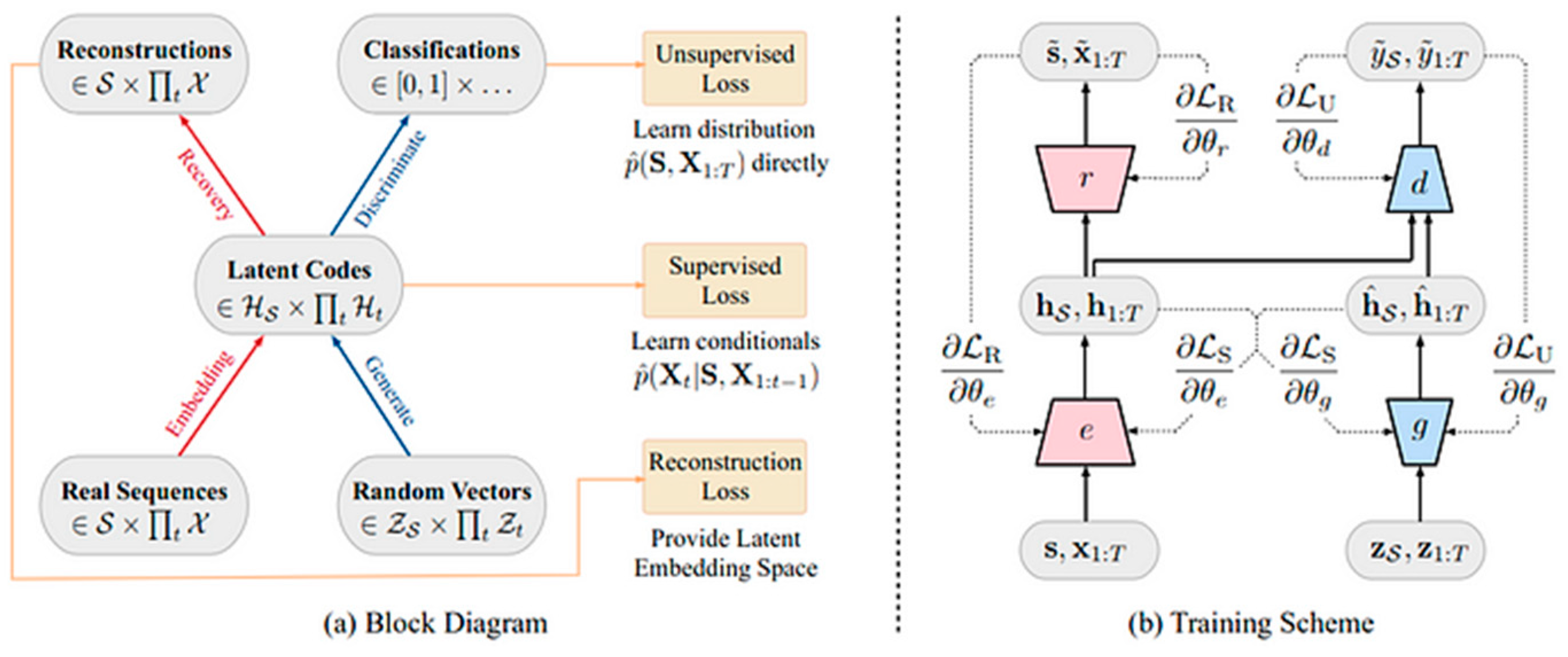
Figure 1. TimeGAN block diagram and training scheme, as depicted in [1].
Stats 07 00049 g001
Figure 2. Probabilistic flood-forecasting model.
Stats 07 00049 g002
Figure 3. PCA and t-SNE visualization with two components for both synthetic- and real-flood-event data by the different GANs, TimeGAN, RTSGAN, and MC-TSGAN.
Stats 07 00049 g003
Figure 4. Six-hour-ahead water-level prediction on the test set using the flood-forecast model trained on augmented and original data.
Stats 07 00049 g004
Figure 5. NSE and KGE for flood forecast time horizons for up to 6 h.
Stats 07 00049 g005
Figure 6. River Ahr streamflow with the marked area used for training the time-series GANs. Flood event “C” (red circle is unseen and extremely high. A and B are the extremes in the training and validation set).
Stats 07 00049 g006
Table 1. Discriminative and predictive scores of MC-TSGAN, TimeGAN, and RTSGAN.
ScoreTimeGANRTSGANMC-TSGAN
Discriminative0.102 (0.021)0.054 (0.024)0.0490 (0.0185)
Predictive0.088 (0.001)0.067 (0.030)0.0519 (0.0474)
Table 2. Probabilistic model results in terms of CRPS, MPIW, and PICP when trained on original and augmented dataset.
Metric
(6th Hour Ahead)
Augmented with MC-TSGANOriginal Data
CRPS0.375(0.023)0.576 (0.024)
MPIW0.43 (0.021)0.56 (0.02)
PICP0.9210.941
Disclaimer/Publisher’s Note: The statements, opinions and data contained in all publications are solely those of the individual author(s) and contributor(s) and not of MDPI and/or the editor(s). MDPI and/or the editor(s) disclaim responsibility for any injury to people or property resulting from any ideas, methods, instructions or products referred to in the content.