Article

Patent Keyword Analysis Using Bayesian Zero-Inflated Model and Text Mining

Department of Data Science, Cheongju University, Cheongju 28503, Chungbuk, Republic of Korea
Stats 2024, 7(3), 827-841; https://doi.org/10.3390/stats7030050
Submission received: 27 June 2024 / Revised: 25 July 2024 / Accepted: 30 July 2024 / Published: 3 August 2024

Abstract

:
Patent keyword analysis is used to analyze the technology keywords extracted from collected patent documents for specific technological fields. Thus, various methods related to this type of analysis have been researched in the industrial engineering fields, such as technology management and new product development. To analyze the patent document data, we have to search for patents related to the target technology and preprocess them to construct the patent–keyword matrix for statistical and machine learning algorithms. In general, a patent–keyword matrix has an extreme zero-inflated problem. This is because each keyword occupies one column even if it is included in only one document among all patent documents. General zero-inflated models have a limit at which the performance of the model deteriorates when the proportion of zeros becomes extremely large. To solve this problem, we applied a Bayesian inference to a general zero-inflated model. In this paper, we propose a patent keyword analysis using a Bayesian zero-inflated model to overcome the extreme zero-inflated problem in the patent–keyword matrix. In our experiments, we collected practical patents related to digital therapeutics technology and used the patent–keyword matrix preprocessed from them. We compared the performance of our proposed method with other comparative methods. Finally, we showed the validity and improved performance of our patent keyword analysis. We expect that our research can contribute to solving the extreme zero-inflated problem that occurs not only in patent keyword analysis, but also in various text big data analyses.

1. Introduction

Patent analysis is a very popular approach for the management of technology (MOT), such as new product development, technology innovation, and research and development (R&D) planning. Many researchers have attempted to derive the insights necessary from the results of patent analyses for MOT [1,2,3]. Most patent analysis studies focus on the analysis of the relationships between the keywords included in patents [1,4,5]. This method analyzes the patent keywords extracted from the searched patent documents related to the target technology. Generally, patent keyword data are analyzed using statistical and machine learning algorithms. For analyses based on statistics and machine learning, the patent documents must be transformed into structured data, such as a patent–keyword matrix [1,5]. In this matrix, the patent document and keywords are assigned to the row and column, respectively. Each element of the matrix is the frequency value of a keyword that has occurred in a patent document. In general, most elements of the matrix are zero. This is because a keyword included in only one document among all patent documents requires an entire column. Thus, in patent keyword analysis, we encounter the extreme zero-inflated problem. This problem is a major cause of the deteriorating performance of prediction models for patent keyword analysis.
Until now, various data analysis methods have been studied to solve the zero-inflated problem [6,7,8,9,10,11,12,13,14,15,16,17,18]. These have mainly been probability models based on mixture distributions using Bernoulli, Poisson, and negative binomial distributions. Zero-inflated probability models are built by dividing them into a part where many zero values occur and a part where non-zero observed values occur. Therefore, they have a structure that is a mixture of two different models. One is the zero-inflated binomial part, and the other is the count Poisson part. Bayesian modeling is another approach to zero-inflated data analysis. Many researchers have studied Bayesian models to solve the zero-inflated problem in various fields. Oganisian et al. (2021) proposed a Bayesian nonparametric model for zero-inflated data analysis [10]. They applied their proposed Bayesian model to pathological data for prediction, clustering, and causal estimation. Lee et al. (2020) studied Bayesian variable selection for multivariate zero-inflated models, and they also focused on biology in terms of microbiome count data [11]. Hwang (2022) applied a Bayesian joint model to analyze zero-inflated count data in developmental toxicity studies [12]. He also considered the zero-inflated model with Poisson distribution and Monte Carlo simulation. In addition, various studies using Bayesian inference have been conducted to solve the zero-inflated problem [13,14,15,16,17].
However, when the proportion of zeros becomes extremely large, exceeding half of the total data, there are limits to analyzing it with a general zero-inflated model [4,5]. Therefore, we need another approach to solve the extreme zero-inflated problem that occurs in patent keyword analysis. We conducted a patent keyword analysis that applies Bayesian inference to a general zero-inflated model to overcome the extreme zero-inflated problem. In this paper, we propose a method of patent keyword analysis using a Bayesian zero-inflated model and text mining. Using text mining techniques, we constructed a patent–keyword matrix as the structured data. Also, we analyzed the matrix using a Bayesian zero-inflated model.
In the next section, we discuss the research background, such as text mining for patent data and zero-inflated count modeling. The proposed method for the patent keyword analysis is shown in Section 3. Our experimental results are presented in Section 4. In that section, we explain the theoretical and practical issues related to our proposed method and experimental results. Following that is a discussion section that explains the effectiveness of the proposed model and how it is used in real applications. The conclusions of our research and possible future works are described in the last section.

2. Research Background

2.1. Text Mining for Patent Data

To analyze patent keywords, we built structural data from patent documents using text mining [1,19]. We searched the patents related to the target technology from patent databases around the world. Patent documents contain a variety of information on a developed technology, such as the patent title, abstract, inventors, claims, technological codes, citations, issued date, drawings, etc. [5]. Thus, using the patent analysis, we can find valuable results for the MOT. The process of text mining for patent data is represented as follows.
In Figure 1, the first step was to search the patent documents related to the target technology in the patent databases. The collected patent data were unstructured. Thus, we preprocessed the patent documents to be transformed into structured data. In this step, we used various text mining techniques such as data import, text cleanup, tokenization, corpus, filtering, stemming, etc. [19]. Next, we created a patent–keyword matrix using the keywords extracted from the structured data. This matrix comprised the frequency with which a keyword occurred in each patent document. In this case, a zero-inflated problem occurs because a significant portion of the matrix elements have the value of zero. This problem causes the performance of the analysis model to deteriorate. To solve this problem, many studies have been conducted in the fields of statistics and machine learning [4,6,7,8,18,20,21]. Lastly, we construct a patent analysis model analyzing the patent–keyword matrix using statistics and machine learning algorithms. Therefore, we need a more advanced model to analyze the zero-inflated data from the patent documents. In the next section, we illustrate the zero-inflated count models for analyzing the patent–keyword matrix with zero inflation.

2.2. Zero-Inflated Count Model

To analyze the count data, such as the frequency of patent keywords, we use the generalized linear model (GLM) with Poisson and binomial distributions [22,23,24]. For example, the Poisson linear regression model is represented as follows.
log λ = β 0 + β 1 x 1 + β 2 x 2 + + β p x p
In Equation (1), the link function of Poisson regression is log function. λ is the Poisson parameter representing the average number (rate) of occurrences. In addition, the negative binomial regression is a widely used model for analyzing count data [25,26]. In count data, we use the Poisson distribution if the mean and variance of the random variable are similar; otherwise, we use the negative binomial distribution [27]. The count data models make it difficult to properly analyze the data if the given data contain excessive zeros [4,21]. The problem of zero-inflated data was introduced by Lambert (1992) [28]. As the proportion of zeros in the given data increases, the influence of zeros in the process of building an analysis model increases. In other words, when zero-inflated data are analyzed using a general statistical model, the performance of the constructed model deteriorates. For example, the coefficient of determination ( R 2 ) of a regression model for zero-inflated data becomes very small and the AIC value becomes very large, making the constructed model unusable [4,21]. Consequently, we need research on ways to solve the zero-inflated problem.
In general, the zero-inflated model is a statistical model analyzing the count data with zero inflation [4,8,20,21,25,26,27,28]. We assume that zero occurs for two reasons in the zero-inflated model [27]. The first is a structural zero generated from the binomial distribution and the second is a random zero generated from the Poisson distribution. So, the zero-inflated model consists of two components [26,27]. The first one is the zero-inflated component. This component models the excess zeros in the data. The second one is the count component. This deals with the non-zero counts in the data, and follows a count distribution such as Poisson or negative binomial. The zero-inflated models are commonly used in various fields, including epidemiology, ecology, medicine, health care, and toxicity, where count data with excess zeros are frequently encountered [8,9,14,15,20]. They allow the modeling of both the probability of observing a zero count and the distribution of non-zero counts simultaneously. The zero-inflated model is defined as Equation (2) [27].
P Y = y = w + 1 w f 0 , y = 0 1 w f y ,   y > 0
where f · is a probability distribution function. In the zero-inflated Poisson (ZIP) model, the function is the probability mass function of the Poisson random variable, as follows [28].
f y = e λ λ y y ! ,   y = 0 , 1 , 2 ,
In Equation (3), λ is the parameter of Poisson distribution and represents the mean value of occurred events. Also, we use the negative binomial distribution for f · in the zero-inflated negative binomial (ZINB) model [26]. To date, the research addressing the issue of zero inflation has been conducted across a spectrum of disciplines, including statistics and machine learning [4,6,7,21,22]. Park and Jun employed the compound Poisson model as a methodological approach to mitigate the zero-inflated challenge encountered in the analysis of patent data [5]. They partitioned the provided dataset into zero and non-zero areas, subsequently employing compound Poisson and gamma distributions. Hilbe (2011) explained the ZIP and ZINB to overcome the sparsity of zero inflation in count data analysis [26,27]. Jun (2024) tried to deal with the zero-inflated problem using the generative adversarial network (GAN) as a deep learning [22]. In addition, several studies that introduced Bayesian statistics to handle the zero-inflated problem have been conducted [6,7,9,29]. Neelon and Chung (2017) used Bayesian inference and the latent factor model to analyze zero-inflated count data using Markov Chain Monte Carlo (MCMC) and data augmentation [7]. In the next section, we explain our proposed method for patent keyword analysis.

3. Proposed Method for Patent Keyword Analysis

Patent keyword analysis is used to analyze the relations between the patent keywords using statistics and machine learning algorithms. The main purpose of patent keyword analysis is to identify relationships between detailed technologies in a specific technological field and generate the knowledge necessary for MOT. For example, we use the analysis results to identify core technologies, survey technological development trends in the market, establish R&D strategies, perform intellectual property management, develop new products, achieve technological innovation, and forecast future technology. To generate patent keyword data for the target technology, we extract the title and abstract from each collected patent document. Using the text mining techniques, we preprocess the title and abstract data to construct the patent–keyword matrix, as follows [20].
  • (Step 1) Data import: cleaning up and structuring the input text for further works
  • (Step 2) Stemming: removing word suffixes to the root form
  • (Step 3) Whitespace elimination: erasing white space
  • (Step 4) Lowe case conversion: converting the words to lower case
  • (Step 5) Stopwords removal: removing common words used in most patents
In Step 1, we import the patent documents collected from various patent databases. Next, through Steps 2 to 5, the suffix of each word is erased, white spaces are removed, all words are changed to lowercase, and stopwords that are not necessary for keyword analysis are removed. Using the preprocessing results from Steps 1 to 5, we perform the following five class buildings to construct the patent–keyword matrix for patent keyword analysis [20].
  • (Class 1) Corpus: patent document collection, a database for patent documents
  • (Class 2) Patent text document: each patent managed by patent document collection
  • (Class 3) Patent text repository: a repository used for tracking patent collections
  • (Class 4) Patent-keyword matrix: a bag of words for further patent keyword analysis
Starting with creating a corpus class, classes for patent text documents and patent text repositories are built, and finally a patent–keyword matrix class is constructed. We analyze this matrix in the patent keyword analysis. In this paper, we propose a statistical method to analyze the patent keyword data with zero inflation. To analyze the zero-inflated keyword data, we use the Bayesian ZIP regression model combining Bayesian inference and ZIP modeling.
The existing ZIP regression model estimates parameters using the maximum likelihood estimation (MLE) method. If the sample size is large enough and the percentage of zero inflation is not large, the parameters estimated by MLE are efficient estimators. However, if the sample size is small or the percentage of zero inflation is large, especially when the percentage of zero inflation becomes greater than 50%, the parameters estimated by MLE are no longer efficient. This is because the likelihood function defined as follows depends on the size n of the observed data [29].
L θ | y = i = 1 n f y i | θ
where θ is the parameter and y represents the observed data. In general, we estimate θ , which maximizes the likelihood function in Equation (4). In addition, because the likelihood function depends 100% on the observed data, if y contains too many zeros, the estimation process for θ is also overly influenced by zeros, so it is difficult to efficiently estimate θ . For example, the MLE of the parameter of the Poisson distribution is the mean of the observed data. This is dependent on the zero values in the observed data. To solve this problem, we study a method able to analyze patent keywords by applying Bayesian inference to ZIP. In the Bayesian ZIP model, because we use the prior distribution for θ , the parameter estimation process does not completely depend on the observed data.
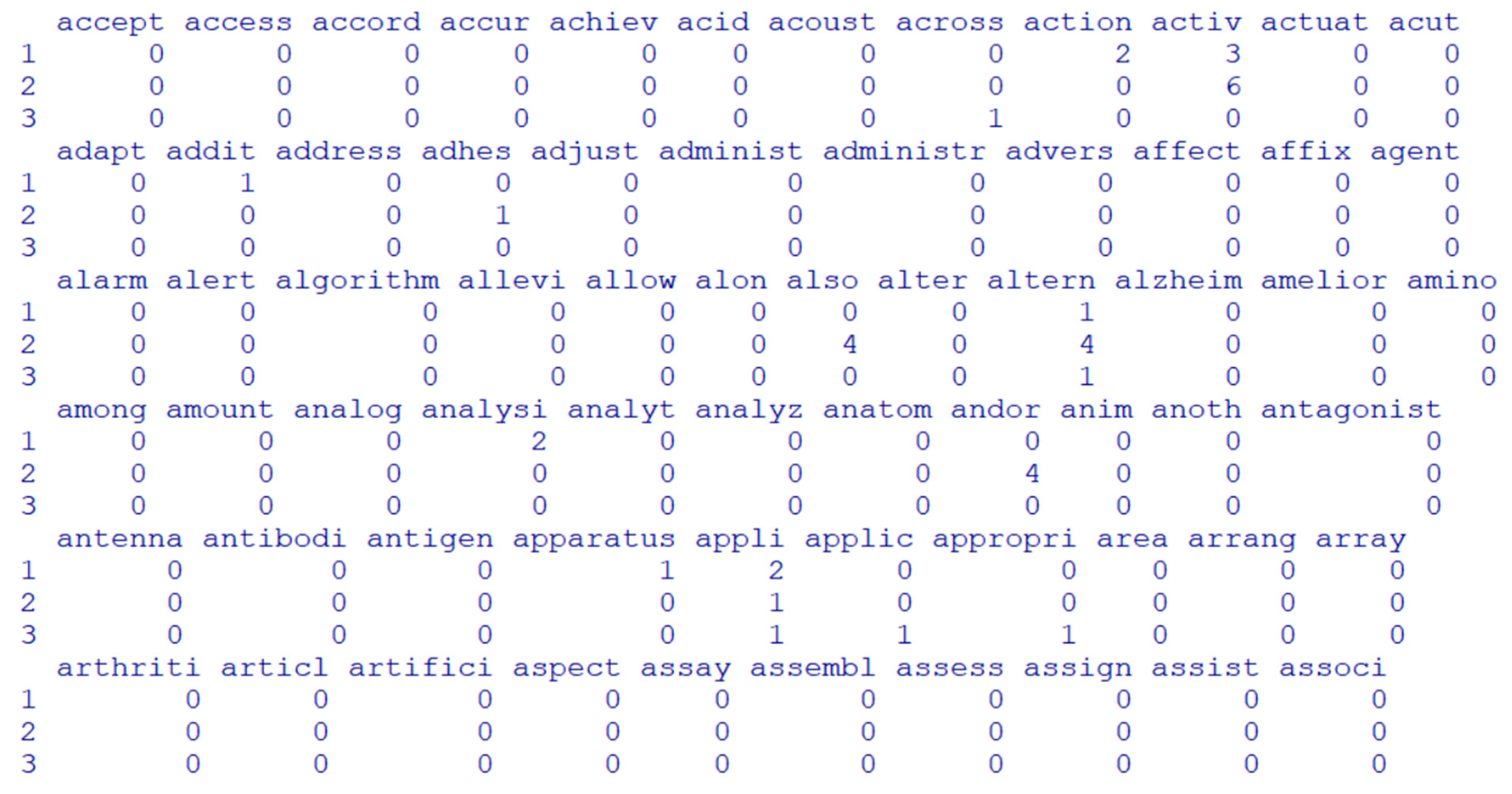
The proposed method consists of a text mining step to preprocess the collected patent documents and a Bayesian zero-inflated modeling step to analyze the preprocessed patent keyword data. First, using the search equation for target technology, we retrieve the patent documents related to target technology from patent databases such as the United States Patent and Trademark Office (USPTO) and the Korea Intellectual Property Rights Information Service (KIPRIS) [30,31]. We chose digital therapeutics as our target technology. Recently, various research and developments in digital therapeutics are actively underway in the healthcare field. To analyze the patent documents, we preprocess the document data using text mining. Using text mining techniques such as corpus and parsing, we extract technology keywords from the retrieved patent documents. In addition, we construct the patent–keyword matrix from the extracted keywords. The patent–keyword matrix constructed by our patent keywords is shown in Figure 2.
Figure 2 shows a part of the entire patent–keyword matrix. Each column and row represent a keyword and a document, respectively, and the elements of this matrix are the number of keywords included in the patent document. As can be seen in Figure 2, most elements in the patent–keyword matrix generally have the value of zero. This is due to the characteristics of the patent–keyword matrix, where the size of columns is larger than the rows. In other words, even if a keyword is included in only one patent document among all patent documents, it occupies one column in the matrix. This zero-inflated problem is a major cause of the deterioration of the performance of prediction models based on statistics and machine learning. In order to solve the zero-inflated problem of patent keyword data, in this paper, we propose patent keyword analysis using a Bayesian ZIP regression model. Next, we explain our proposed model based on Bayesian ZIP for patent keyword analysis.
The ZIP distribution is used when more zeros are observed than occur under the assumption of the Poisson distribution. If the data that follow the ZIP distribution are modeled using the general Poisson distribution, a biased estimation occurs for the zero-inflated portion, degrading the performance of the prediction model. The ZIP model assumes that zero occurs for two reasons. The first is a structural zero that occurs from a binomial distribution and the second is a random zero that occurs from a Poisson distribution. The probability mass function (pmf) of the response variable Y in the ZIP regression model consisting of P explanatory variables is shown in Equation (5) [28,29].
P Y = y | w , λ = w + 1 w p ( y | λ ) , y = 0 1 w p ( y | λ ) ,   y > 0
where w is the probability of zero occurrence and λ represents the Poisson parameter along with x . The Poisson probability function in Equation (5) is defined as follows [32]:
p y | λ = e λ λ y y ! ,   y = 0 , 1 , 2 ,
In Equation (6), the Poisson parameter is defined as the predictor, e X β . The ZIP model builds a regression model consisting of two parts, binomial zero inflation ( w ) and the Poisson count ( λ ). First, the regression model for w is defined as follows [33]:
log w 1 w = τ 0 x 0 + τ 1 x 1 + τ 2 x 2 + + τ q x q = X w τ
In Equation (7), q is the number of explanatory variables (covariates) used to predict w of the binomial model in ZIP and x 0 is 1 in (7). Next, the ZIP regression model for λ is as follows [33]:
log λ = β 0 x 0 + β 1 x 1 + β 2 x 2 + + β p x p = X λ β
In Equation (8), p is the number of explanatory variables used to predict λ of the Poisson model in ZIP. q and p may be the same or different. In other words, the list of explanatory variables used in the binomial model and Poisson model included in ZIP may be the same or different. Therefore, in the ZIP regression model, w and λ appear as Equation (9).
w = 1 1 + e X w α ,   λ = e X λ β
The final regression model can be expressed as Equation (10) [12,28]:
P Y = y | α , β = 1 1 + e X w α + 1 1 1 + e X w α e e X λ β , y = 0 1 1 1 + e X w α e e X λ β e X λ β y y ! ,   y > 0
In the ZIP regression model, the regression coefficient is estimated using the MLE method, but if the zero ratio becomes extremely large, the performance of the model deteriorates [4,9,19,22]. To solve this problem, we use a Bayesian ZIP regression model that applies Bayesian inference to the ZIP regression model. The likelihood function in the Bayesian ZIP model is as follows [12,28].
L Y | α , β = i = 1 n 1 1 + e X w α + 1 1 1 + e X w α e e X λ β S i × i = 1 n 1 1 1 + e X w α e e X λ β e X λ β y y ! 1 S i
In Equation (11), n is the data size and S i is the indicator function in Equation (12).
S i = 1 , y i = 0 0 , y i > 0
Therefore, the likelihood function is divided into zero states and non-zero states based on S i . Next, we use the normal distribution as the prior distribution for α and β in Equation (13) [12,28]. This is because the coefficients of a regression model can take on a whole range of real numbers.
f α , β | μ α , μ β , σ α , σ β = j = 0 q 1 2 π σ α e α j μ α 2 2 σ α 2 × k = 0 p 1 2 π σ β e β k μ β 2 2 σ β 2
Using the previous likelihood function and prior distribution, we obtain the posterior distribution, as follows [12,28]:
f α , β | Y = i = 1 n 1 1 + e X w α + 1 1 1 + e X w α e e X λ β S i × i = 1 n 1 1 1 + e X w α e e X λ β e X λ β y y ! 1 S i
× j = 0 q 1 2 π σ α e α j μ α 2 2 σ α 2 × k = 0 p 1 2 π σ β e β k μ β 2 2 σ β 2
We estimate the model parameters using the posterior distribution obtained in Equation (14). In fact, when the model is complex or the number of parameters is large, parameter estimation becomes difficult and we perform posterior inference using the MCMC method. Therefore, we carry out the patent keyword analysis using the Bayesian ZIP regression model to overcome the limitations of the Poisson and ZIP models related to the zero inflation problem. Figure 3 shows the entire process of our proposed patent keyword analysis, from collecting patent documents to the patent keyword analysis.
For the patent keyword analysis, we transform the searched patent documents into a patent–keyword matrix using text mining techniques. In this way, an extreme zero-inflated problem occurs in the preprocessed patent keyword data. This is a major cause of the deterioration of the performance of prediction models in patent keyword analysis. This problem cannot be solved even with a general zero inflation model such as ZIP. To solve this extreme zero inflation problem, we propose the performance of patent keyword analysis using the Bayesian ZIP model, which applies Bayesian inference to the ZIP model.
To compare the performance of models such as Poisson regression, ZIP and Bayesian ZIP, we use the interval estimation of model parameters. We compare the range of estimated intervals for the regression coefficients of each model. In order to obtain the interval range for comparing model performance, we divide the interval range of the parameter into Bayesian and non-Bayesian cases. First, in the case of non-Bayesian models such as Poisson regression and ZIP, we estimate the 100(1 − α ) % confidence interval of the regression coefficient using Equation (15) [29].
θ ^ ± t α / 2 , n 2 S E θ ^
where α is the significance level valued from 0 to 1 and S E θ ^ is a standard error of θ ^ . Next, in the Bayesian ZIP, we use the highest posterior density (HPD) interval for the interval range. The 100(1 − α ) % HPD interval for θ is defined as follows [33]:
P θ L < θ < θ H | y = 1 α
In Equation (16), θ L and θ H are the lower and upper bounds of the HPD interval, respectively. In addition, P θ i | y is larger than P θ j | y if θ i θ L , θ H and θ j θ L , θ H . Although the confidence interval of the frequentist and HPD interval of the Bayesian model are different, we used two intervals because we were comparing the range of the 95% interval for the mean of the estimated parameter. In Bayesian inference, the final information about θ is in the posterior distribution, so the interval estimate also depends on the posterior distribution. If the interval has the same confidence level, we estimate the interval containing many θ values with a high posterior density function. In practice, it is difficult to accurately obtain the posterior distribution of θ , so the Bayesian HPD interval is obtained using Markov Chain Monte Carlo (MCMC) as follows [29,33].
  • (Step 1) Sampling θ * from Q θ | θ t 1
  • (Step 2) Computing acceptance probability
    α = min 1 , P θ * | y P θ t 1 | y Q θ t 1 | θ * Q θ * | θ t 1
  • (Step 3) Selecting θ t
    u ~ U 0 , 1 θ t = θ * u α θ t 1 u > α
In Step 1, we obtain a new sample θ * from the density of Q θ | θ t 1 at time (t − 1). Next, we compute the acceptance probability of θ * in Step 2. Finally, we decide whether to choose θ * by comparing the acceptance probability obtained in Step 2 with the value randomly drawn from the uniform distribution, U 0 , 1 . The generated samples must be independent of each other. However, because MCMC generates new samples using previous results, the samples are dependent on each other. Moreover, warm-up time is required for the samples to converge to the posterior distribution. To deal with this problem, we perform the task of burn in, discarding samples initially generated during the sampling process using MCMC. We construct the HPD interval using the MCMC for model comparison. In the next section, we perform the experiments using the practical patent data to compare the performance of Bayesian ZIP with Poisson regression and ZIP models.

4. Experiments and Results

To compare the performance of the proposed method, we collected patent documents related to digital therapeutics technology and used them in our experiments. We compared the model performance of Bayesian ZIP regression with Poisson and ZIP regression. In particular, we evaluated the performance of each model using the 95% confidence interval (CI) for the regression coefficient of each model. The CI for the regression coefficient β refers to the set C that satisfies the following equation, given the observed value x of X [34].
P β C | X = x = 1 α
In Equation (17), α is the significance level and has a value between 0 and 1. In this paper, we set α as 0.05 (95% CI) to obtain the CI and used it to evaluate the performance of comparative models. In particular, since most information about parameter β in Bayesian inference is considered to be summarized in the posterior distribution, we also obtained the interval estimation based on the posterior distribution. Also, we performed our experiments using R data language and its packages [20,35,36].

4.1. Text Mining for Constructing Patent-Keyword Matrix

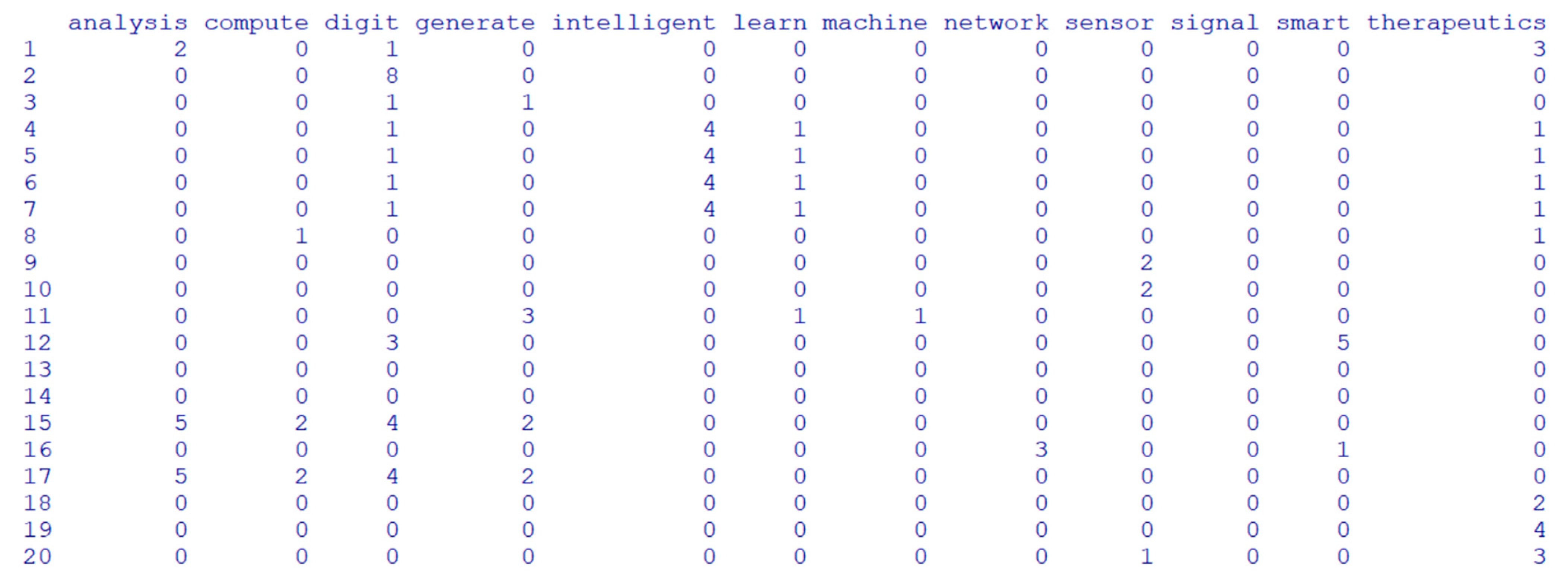
To perform the patent keyword analysis, we searched the patent documents related to digital therapeutics technology from the USPTO and KIPRIS [30,31]. Through the valid patent selection process, we finally selected 2,685 patent documents. Using the text mining techniques, we extracted 675 patent keywords from the text database. Among them, we selected 12 technology keywords as follows: ‘analysis’, ‘compute’, ‘digit’, ‘generate’, ‘intelligent’, ‘learn’, ‘machine’, ‘network’, ‘sensor’, ‘signal’, ‘smart’ and ‘therapeutics’. Figure 4 shows the patent–keyword matrix for our patent keyword analysis using the Bayesian ZIP regression model.
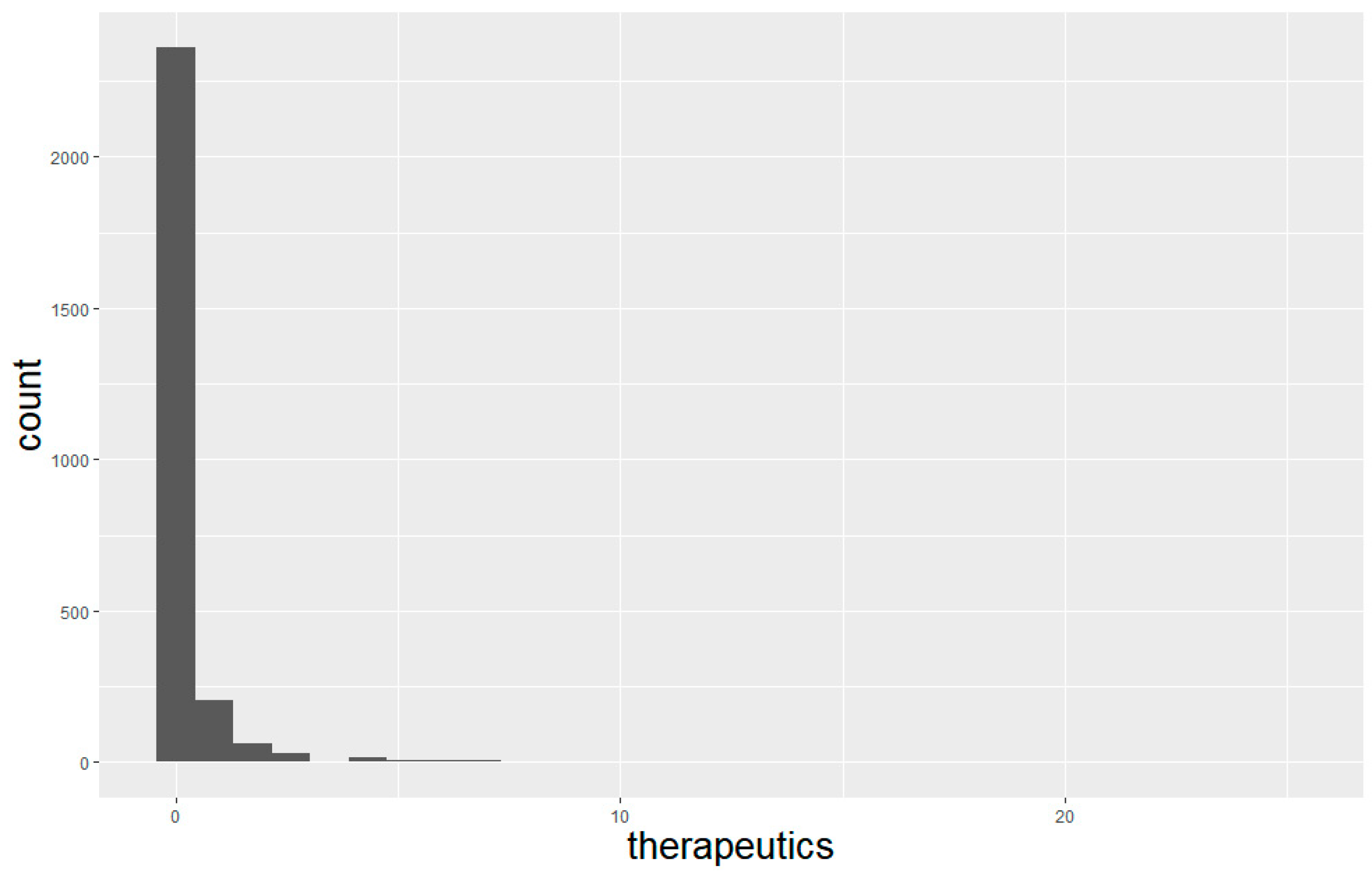
Using the patent–keyword matrix in Figure 4, we performed the patent keyword data analysis. In our experiment, we used the keyword ‘therapeutics’ as a response variable in the regression model. In addition, we used the keywords ‘analysis’, ‘compute’, ‘digit’, ‘generate’, ‘intelligent’, ‘learn’, ‘machine’, ‘network’, ‘sensor’, ‘signal’ and ‘smart’ as explanatory variables to explain the response keyword. Figure 5 shows the frequency distribution of the response keyword therapeutics.
In Figure 5, we can see that most frequency values were zeros. That is, these data have a zero-inflated problem. The zero ratio of the response variable ‘therapeutics’ is 87.86%. In the next section, we use the Bayesian ZIP regression model to solve the extreme zero-inflated problem that appeared in the patent keyword analysis.

4.2. Patent Keyword Data Analysis Using Bayesian ZIP Regression Model

For the performance comparison, we compared the Bayesian ZIP regression model with the general Poisson and ZIP regression models. The response variable of the regression model is the keyword ‘therapeutics’, and all other keywords are used as explanatory variables. First, we built the general Poisson regression model. This regression model is based on Poisson distribution, as follows [28].
f y i | X i = e λ i λ i y i y i ! ,   y i = 0 , 1 , 2 , ,   2685
In Equation (18), y is the response keyword ‘therapeutics’ and X is the random vector of explanatory keywords (analysis, compute, digit, generate, intelligent, learn, machine, network, sensor, signal, smart). λ i is the parameter of Poisson distribution and represents the occurrence rate (mean) of an event. i is an index of the data size from 1 to n. The regression equation derived from Poisson distribution is defined as follows [28].
l o g λ i = X i β
In Equation (19), β is the regression coefficient vector corresponding to X . This is a generalized linear model (GLM) with Poisson distribution and a log link function. Therefore, we construct the predictive model of y given X .
E y i | X i = e x p X i β
We predict the expected frequency using the exponential function of the linear predictor of X i β in Equation (20). Table 1 shows the analysis results of the Poisson regression model.
In Table 1, we show the p-values and regression coefficients of the explanatory keywords. In addition, we can build the 95% confidence interval of the coefficient using the value of 2.5% (lower) and 97.5% (upper). In the Poisson regression model, we found that the variables of ‘keywords’, ‘intelligent’, ‘machine’, ‘sensor’ and ‘signal’ statistically significantly explain the response variable of the keyword ‘therapeutics’. To compare the model performance of the Poisson GLM with the ZIP regression model, we show the results of te ZIP regression model in Table 2.
In Table 2, the results of the ZIP model consist of two parts: count and zero-inflation models. The count model is based on the Poisson distribution with log link function, and the zero-inflation model is also based on binomial distribution with the logit link function. In the zero-inflated binomial part, we found that the keyword ‘generate’ is significant because its p-value is less than 0.05. In addition, we knew that the keywords ‘analysis’, ‘compute’, ‘generate’, ‘intelligent’, ‘learn’, ‘machine’, ‘network’ and ‘sensor’ have p-values less than 0.05 in the count Poisson part. Therefore, we could see that these keywords were statistically significant. We also confirmed that the keywords ‘intelligent’, ‘machine’ and ‘sensor’ appear significantly in both the general Poisson model and the Poisson (count) model of ZIP. Unlike the analysis results for the Poisson model, we found that the absolute values of the coefficients of the keywords ‘learn’ and ‘machine’ in the ZIP model were very large compared to other keywords. Additionally, we found that the difference between their 2.5% and 97.5% percentiles for the regression coefficient was very large compared to other keywords. Through this, we were able to see that the ZIP model also shows limitations when the proportion of zero in the given data is very large. To overcome this limitation, we used the Bayesian ZIP model to analyze patent keyword data. Next, we show the results of the patent keyword analysis using the Bayesian ZIP regression model in Table 3.
In this experiment, we specified the number of MCMC generations as 2000. We illustrate the mean, median, 2.5% and 97.5% percentiles of the regression coefficients of explanatory keywords. From Table 3, we can see that the difference between 97.5% and 2.5% in the binomial distribution part is very small. We also found that the width of the 95% confidence interval (CI) in the Poisson distribution part of Bayesian ZIP was calculated to be smaller than that in the Poisson part of the ZIP model. Also, we selected 2,000 as the burn-in times of the MCMC computing. Table 4 shows the results of comparing the width of the 95% CI between the three models: Poisson, ZIP, and Bayesian ZIP.
We found that the 95% CI width of the Bayesian ZIP regression model is the smallest among the compared models in Table 4. We compared the 95% CI results of the three comparative models with the occurrence frequency of explanatory keywords in patent documents. Table 5 represents the frequency with which each keyword occurred in patent documents.
The zero ratio of each keyword is as follows: analysis (94.00%), compute (90.73%), digit (98.03%), generate (87.41%), intelligent (97.58%), learn (96.24%), machine (96.69%), network (94.86%), sensor (91.58%), signal (94.38%), smart (98.32%), therapeutics (87.86%). Therefore, we can see that the given patent keyword data are very zero-inflated. In other words, they are beyond the level of zero inflation that can be handled in a general ZIP model. In this paper, we applied the Bayesian ZIP model to solve the severe zero-inflated problem that occurs in patent keyword data. From the comparison results in Table 4, we illustrated that the performance of Bayesian ZIP is better than other models such as Poisson regression and ZIP.

5. Discussion

In this paper, we studied a patent keyword analysis method able to deal with the zero-inflated problem. Zero inflation is a problem that must be solved because it seriously reduces the performance of data analysis models. Existing zero-inflated models for analyzing zero-inflated data, such as ZIP and ZINB, have provided effective performance in zero-inflated data analysis. However, the patent–keyword matrix data constructed by preprocessing the patent documents we collected have an extreme zero-inflated data structure that contains an excessively large number of zero values. Therefore, we applied Bayesian inference to the ZIP for analyzing the patent–keyword matrix. From our experimental results, we were able to confirm that the Bayesian ZIP performed better than the existing ZIP in the extremely zero-inflated data.
The Bayesian ZIP is used to deal with the zero-inflated problem that occurs in patent–keyword matrix data and to reduce the interval width of the regression coefficient. Therefore, we made it possible to analyze patent keyword data that provide improved performance for the data containing many zero values. We can use the proposed model in various real applications. Our practical application in this paper was in the field of digital therapeutics technology. When applying the proposed model to a real problem, we first determined the target technology and searched for related patent documents. Next, we constructed a patent–keyword matrix through preprocessing using text mining techniques. Using the Bayesian ZIP, we analyzed the matrix and found the relationships between the patent keywords. The results of the patent keyword analysis can be used for diverse MOT areas. For example, we can construct technology diagrams or trees, develop R&D strategies, develop new products, achieve technological innovation, etc., using the results of patent keyword analysis.

6. Conclusions

We proposed a patent keyword analysis method using a Bayesian ZIP regression model to solve the extreme zero-inflated problem in the patent–keyword matrix. Using text mining techniques, we preprocessed the collected patent documents to build the patent–keyword matrix. This matrix consists of patent documents and technology keywords in its rows and columns, respectively. Each element of the matrix represents the frequency with which a keyword occurred in a patent. Most of the elements are zero values. This is because, even if a keyword is included in only one patent among all patent documents, it will have one column. Therefore, we have to solve this zero-inflated problem for technology keyword analysis using statistical models and machine learning algorithms.
In general, we used the ZIP regression model for zero-inflated data analysis. However, when the proportion of zeros in the given patent keyword data became extremely large, we found that the performance of the general ZIP model deteriorated in our experimental results. We analyzed the patent–keyword matrix with extreme zero inflation using the Bayesian ZIP model, and showed that the performance of Bayesian ZIP is better than Poisson and ZIP models.
In this paper, we applied Bayesian inference to a ZIP model for patent keyword analysis. In particular, we tried to solve the extreme zero-inflated problem contained in patent keyword data. Various models have been proposed to solve the zero-inflated problem, such as zero-truncated Poisson (ZTP), zero-truncated negative binomial (ZTNB) and ZINB. They all have their own advantages and disadvantages in zero inflation data analysis. Thus, we will study diverse Bayesian inference models to improve the performance of traditional zero-inflated models for extreme zero-inflated data analysis in our future works. We also applied hybrid Monte Carlo computing to construct the Bayesian inference models for zero-inflated patent data analysis.

Funding

This research received no external funding.

Institutional Review Board Statement

Not applicable.

Informed Consent Statement

Not applicable.

Data Availability Statement

The data presented in this study are available upon request from the corresponding author (status: privacy).

Conflicts of Interest

The authors declare no conflicts of interest.

References

  1. Xue, D.; Shao, Z. Patent text mining based hydrogen energy technology evolution path identification. Int. J. Hydrog. Energy 2024, 49, 699–710. [Google Scholar] [CrossRef]
  2. Reher, L.; Runst, P.; Thomä, J. Personality and regional innovativeness: An empirical analysis of German patent data. Res. Policy 2024, 53, 105006. [Google Scholar] [CrossRef]
  3. Coccia, M.; Roshani, S. Path-Breaking Directions in Quantum Computing Technology: A Patent Analysis with Multiple Techniques. J. Knowl. Econ. 2024, 1–34. [Google Scholar] [CrossRef]
  4. Park, S.; Jun, S. Zero-Inflated Patent Data Analysis Using Compound Poisson Models. Appl. Sci. 2023, 13, 4505. [Google Scholar] [CrossRef]
  5. Park, S.; Jun, S. Patent Analysis Using Bayesian Data Analysis and Network Modeling. Appl. Sci. 2022, 12, 1423. [Google Scholar] [CrossRef]
  6. Lu, L.; Fu, Y.; Chu, P.; Zhang, X. A Bayesian Analysis of Zero-Inflated Count Data: An Application to Youth Fitness Survey. In Proceedings of the Tenth International Conference on Computational Intelligence and Security, Kunming, China, 15–16 November 2014; pp. 699–703. [Google Scholar]
  7. Neelon, B.; Chung, D. The LZIP: A Bayesian Latent Factor Model for Correlated Zero-Inflated Counts. Biometrics 2017, 73, 185–196. [Google Scholar] [CrossRef] [PubMed]
  8. Yusuf, O.B.; Bello, T.; Gureje, O. Zero Inflated Poisson and Zero Inflated Negative Binomial Models with Application to Number of Falls in the Elderly. Biostat. Biom. Open Access J. 2017, 1, 69–75. [Google Scholar]
  9. Workie, M.S.; Azene, A.G. Bayesian zero-inflated regression model with application to under-five child mortality. J. Big Data 2021, 8, 4. [Google Scholar] [CrossRef]
  10. Oganisian, A.; Mitra, N.; Roy, J.A. A Bayesian nonparametric model for zero-inflated outcomes: Prediction, clustering, and causal estimation. Biometrics 2021, 77, 125–135. [Google Scholar] [CrossRef]
  11. Lee, K.H.; Coull, B.A.; Moscicki, A.-B.; Paster, B.J.; Starr, J.R. Bayesian variable selection for multivariate zero-inflated models: Application to microbiome count data. Biostatistics 2020, 21, 499–517. [Google Scholar] [CrossRef]
  12. Hwang, B.S. A Bayesian joint model for continuous and zero-inflated count data in developmental toxicity studies. Commun. Stat. Appl. Methods 2022, 29, 239–250. [Google Scholar] [CrossRef]
  13. Hajihosseini, M.; Amini, P.; Saidi-Mehrabad, A.; Dinu, I. Infants’ gut microbiome data: A Bayesian Marginal Zero-inflated Negative Binomial regression model for multivariate analyses of count data. Comput. Struct. Biotechnol. J. 2023, 15, 1621–1629. [Google Scholar] [CrossRef] [PubMed]
  14. de Souza, H.C.C.; Louzada, F.; Ramos, P.L.; de Oliveira Júnior, M.R.; Perdoná, G.D.S.C. A Bayesian approach for the zero-inflated cure model: An application in a Brazilian invasive cervical cancer database. J. Appl. Stat. 2022, 49, 3178–3194. [Google Scholar] [CrossRef] [PubMed]
  15. Wanitjirattikal, P.; Shi, C. A Bayesian zero-inflated binomial regression and its application in dose-finding study. J. Biopharm. Stat. 2020, 30, 322–333. [Google Scholar] [CrossRef] [PubMed]
  16. Xie, H.; Rolka, D.B.; Barker, L.E. Modeling County-Level Rare Disease Prevalence Using Bayesian Hierarchical Sampling Weighted Zero-Inflated Regression. J. Data Sci. 2023, 21, 145–157. [Google Scholar] [CrossRef] [PubMed]
  17. Rahmati, M.; Mahmoudi, M.; Mohammad, K.; Mikaeli, J.; Zeraati, H. Bayesian modelling of zero-inflated recurrent events and dependent termination with compound Poisson frailty model. Stat 2020, 9, e292. [Google Scholar] [CrossRef]
  18. Ghosh, S.K.; Mukhopadhyay, P.; Lu, J.-C. Bayesian analysis of zero-inflated regression models. J. Stat. Plan. Inference 2006, 136, 1360–1375. [Google Scholar] [CrossRef]
  19. Feinerer, I.; Hornik, K. Package ‘tm’ Version 0.7-13, Text Mining Package; CRAN of R Project; R Foundation for Statistical Com-puting: Vienna, Austria, 2024. [Google Scholar]
  20. Sidumo, B.; Sonono, E.; Takaidza, I. Count Regression and Machine Learning Techniques for Zero-Inflated Overdispersed Count Data: Application to Ecological Data. Ann. Data Sci. 2023, 11, 803–817. [Google Scholar] [CrossRef]
  21. Jun, S. Zero-Inflated Text Data Analysis using Generative Adversarial Networks and Statistical Modeling. Computers 2023, 12, 258. [Google Scholar] [CrossRef]
  22. Murphy, K.P. Machine Learning: A Probabilistic Perspective; MIT Press: Cambridge, MA, USA, 2012. [Google Scholar]
  23. Theodoridis, S. Machine Learning a Bayesian and Optimization Perspective; Elsevier: London, UK, 2015. [Google Scholar]
  24. Roback, P.; Legler, J. Beyond Multiple Linear Regression: Applied Generalized Linear Models and Multilevel Models in R; CRC Press: Boca Raton, FL, USA, 2021. [Google Scholar]
  25. Hilbe, J.M. Negative Binomial Regression, 2nd ed.; Cambridge University Press: Cambridge, UK, 2011. [Google Scholar]
  26. Hilbe, J.M. Modeling Count Data; Cambridge University Press: New York, NY, USA, 2014. [Google Scholar]
  27. Cameron, A.C.; Trivedi, P.K. Regression Analysis of Count Data, Second Edition; Cambridge University Press: New York, NY, USA, 2013. [Google Scholar]
  28. Lambert, D. Zero-Inflated Poisson Regression, with an Application to Defects in Manufacturing. Technometrics 1992, 34, 1–14. [Google Scholar] [CrossRef]
  29. Hogg, R.V.; McKean, J.M.; Craig, A.T. Introduction to Mathematical Statistics, 8th ed.; Pearson: Upper Saddle River, NJ, USA, 2018. [Google Scholar]
  30. Moriña, D.; Puig, P.; Navarro, A. Analysis of zero inflated dichotomous variables from a Bayesian perspective: Application to occupational health. BMC Med. Res. Methodol. 2021, 21, 277. [Google Scholar] [CrossRef] [PubMed]
  31. USPTO, The United States Patent and Trademark Office. Available online: http://www.uspto.gov (accessed on 1 April 2024).
  32. KIPRIS, Korea Intellectual Property Rights Information Service. Available online: www.kipris.or.kr (accessed on 1 April 2024).
  33. Gelman, A.; Carlin, J.B.; Stern, H.S.; Dunson, D.B.; Vehtari, A.; Rubin, D.B. Bayesian Data Analysis, 3rd ed.; Chapman & Hall/CRC Press: Boca Raton, FL, USA, 2013. [Google Scholar]
  34. Montgomery, D.C.; Peck, E.A.; Vining, G.G. Introduction to Linear Regression Analysis; John Wiley & Sons: Hoboken, NJ, USA, 2012. [Google Scholar]
  35. R Development Core Team. R: A Language and Environment for Statistical Computing, R Foundation for Statistical Computing. Available online: http://www.R-project.org (accessed on 15 May 2023).
  36. Zhang, Q.; Yi, G.Y. Package ‘ZIPBayes’ Version 1.0.2, Bayesian Methods in the Analysis of Zero-Inflated Poisson Model; CRAN of R Project; R Foundation for Statistical Computing: Vienna, Austria, 2022. [Google Scholar]
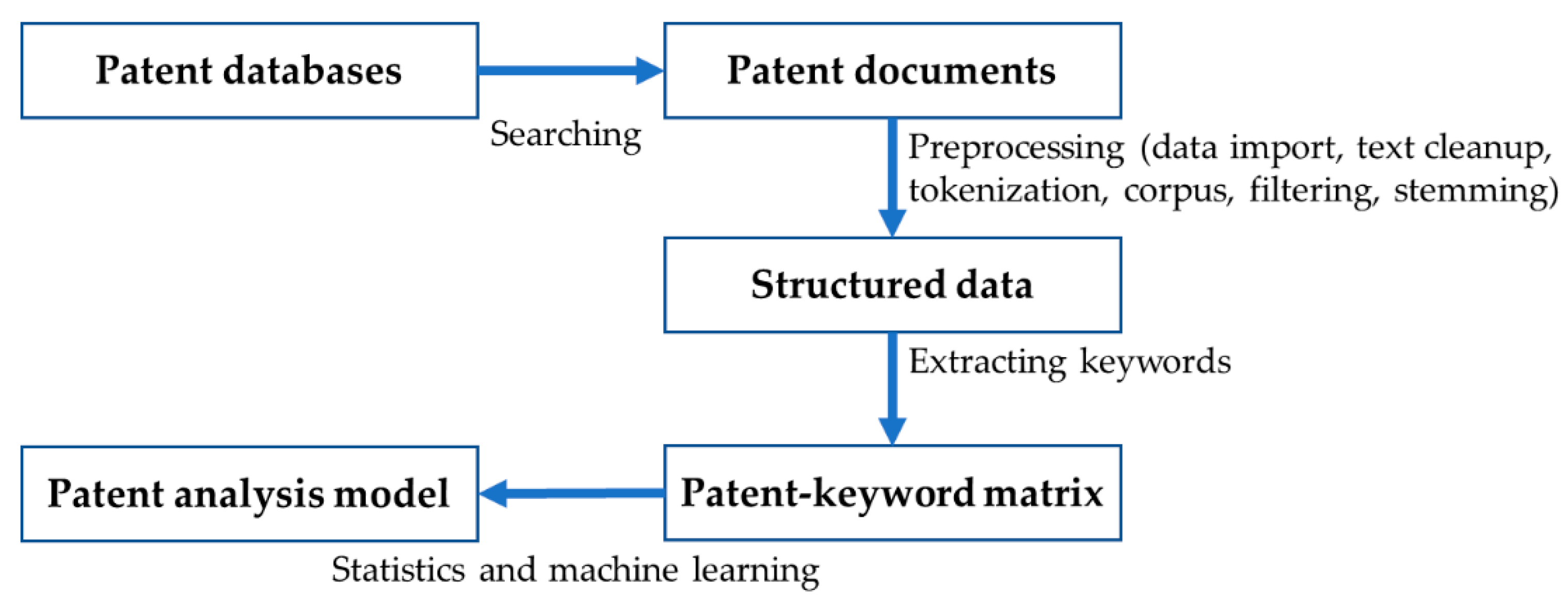
Figure 1. Process of text mining for patent keyword data.
Stats 07 00050 g001
Figure 2. Patent–keyword matrix of digital therapeutics technology.
Stats 07 00050 g002
Figure 3. Process of our proposed patent keyword analysis.
Stats 07 00050 g003
Figure 4. Patent–keyword matrix for our patent keyword analysis.
Stats 07 00050 g004
Figure 5. Frequency distribution of the keyword therapeutics.
Stats 07 00050 g005
Table 1. Results of Poisson regression model.
KeywordPoisson
p-ValueCoefficient2.5%97.5%
analysis0.0710−0.2277−0.4995−0.0023
compute0.36120.0396−0.05250.1231
digit0.6107−0.0850−0.46900.1871
generate0.4939−0.0469−0.18520.0831
intelligent0.00010.40700.18720.5993
learn0.3789−0.2505−0.85780.2559
machine0.0178−1.6314−3.4030−0.5637
network0.0976−0.2186−0.5096−0.0135
sensor0.00020.09940.04350.1468
signal0.00510.13550.04120.2300
smart0.21410.1821−0.16840.4208
Table 2. Results of zero-inflated Poisson regression model.
KeywordBinomialPoisson
p-ValueCoefficient2.5%97.5%p-ValueCoefficient2.5%97.5%
analysis0.0468−0.8504−1.6886−0.01210.0024−0.7012−1.1547−0.2478
compute0.06000.2429−0.01000.49580.00010.31240.16150.4633
digit0.6771−0.2036−1.16120.75410.4680−0.2825−1.04490.4800
generate0.0461−0.3884−0.7701−0.00670.0013−0.3642−0.5859−0.1426
intelligent0.16380.4683−0.19051.12710.00010.71520.36351.0670
learn0.9453−19.9282−4447.30934407.45300.0001−2.3781−3.4261−1.3301
machine0.9932−12.5562−833.8303808.71800.0040−1.9705−3.3110−0.6300
network0.2798−0.1420−0.39930.11530.0136−0.2302−0.4130−0.0473
sensor0.66880.0279−0.09990.15570.00010.24520.11910.3713
signal0.33260.1328−0.13570.40130.27390.1288−0.10180.3595
smart0.98040.0117−0.94510.96860.5902−0.1420−0.65840.3744
Table 3. Results of the Bayesian zero-inflated Poisson regression model.
KeywordBinomialPoisson
MeanMedian2.5%97.5%MeanMedian2.5%97.5%
analysis0.24790.00000.24790.2479−0.99650.1624−1.2947−0.7232
compute0.37040.00000.37040.3704−0.37300.1038−0.5235−0.2348
digit0.68380.00000.68380.6838−0.26410.1468−0.56770.0140
generate0.27830.00000.27830.2783−0.26290.0575−0.3688−0.1047
intelligent−0.10290.1939−0.48310.28300.16840.1324−0.11800.4122
learn0.06380.00000.06370.0638−0.65400.3595−1.4477−0.0427
machine−0.30080.2998−0.88810.1367−2.23960.7230−3.3298−0.5564
network0.81030.00000.81030.8103−0.97700.1705−1.2864−0.6796
sensor0.19470.00000.19470.19470.03450.0295−0.02000.0799
signal0.11270.00000.11270.11270.27770.05590.15960.3512
smart0.46180.00000.46180.4618−0.52290.2187−0.9659−0.1316
Table 4. Comparison of 95% confidence interval width between Poisson, ZIP and Bayesian ZIP.
KeywordPoissonZIPBayesian ZIP
BinomialPoissonBinomialPoisson
analysis0.49721.67650.90690.00000.5715
compute0.17560.50580.30180.00000.2887
digit0.65611.91531.52490.00000.5817
generate0.26830.76340.44330.00000.2641
intelligent0.41211.31760.70350.76610.5302
learn1.11378854.76232.09600.00011.4050
machine2.83931642.54832.68101.02482.7734
network0.49610.51460.36570.00000.6068
sensor0.10330.25560.25220.00000.0999
signal0.18880.53700.46130.00000.1916
smart0.58921.91371.03280.00000.8343
Table 5. Frequency of keywords appearing in each document.
KeywordFrequency
012345>5
analysis25241063113920
compute243612884165214
digit263233114401
generate234719591281653
intelligent262042127400
learn2584771110201
machine2596511910216
network2547892814331
sensor245997762613311
signal2534823319638
smart26403850011
therapeutics2359204632817410
Disclaimer/Publisher’s Note: The statements, opinions and data contained in all publications are solely those of the individual author(s) and contributor(s) and not of MDPI and/or the editor(s). MDPI and/or the editor(s) disclaim responsibility for any injury to people or property resulting from any ideas, methods, instructions or products referred to in the content.