Article

Residual Analysis for Poisson-Exponentiated Weibull Regression Models with Cure Fraction

by
Cleanderson R. Fidelis
1,
Edwin M. M. Ortega
1,* and
Gauss M. Cordeiro
2
1
Department of Exact Sciences, “Luiz de Queiroz” School of Agriculture, University of São Paulo—ESALQ/USP, Piracicaba 13418-900, Brazil
2
Department of Statistics, Centro de Ciências Exatas e da Natureza, Universidade Federal de Pernambuco, Recife 50670-901, Brazil
*
Author to whom correspondence should be addressed.
Stats 2024, 7(2), 492-507; https://doi.org/10.3390/stats7020030
Submission received: 16 April 2024 / Revised: 6 May 2024 / Accepted: 15 May 2024 / Published: 20 May 2024

Abstract

:
The use of cure-rate survival models has grown in recent years. Even so, proposals to perform the goodness of fit of these models have not been so frequent. However, residual analysis can be used to check the adequacy of a fitted regression model. In this context, we provide Cox–Snell residuals for Poisson-exponentiated Weibull regression with cure fraction. We developed several simulations under different scenarios for studying the distributions of these residuals. They were applied to a melanoma dataset for illustrative purposes.

1. Introduction

The application of survival analysis models has expanded substantially in many areas in recent years, such as reliability analysis, operational research, oncology, and tourism, among many other areas. A particular feature of the usual survival models is the assumption that as the measure of the time until the observation of the event of interest approaches infinity, all the observations will involve the occurrence of that event.
However, in many cases, there are individuals (observations) that will not experience the event of interest, where the observed time is considered to be infinity. These models are called survival models with cure fractions. They were first proposed in [1,2,3], which described a population as a mixture of individuals susceptible and other individuals immune to the event under study, assuming that at most one cause contributes to the time until the occurrence of the event of interest for the susceptible individuals, while the immune individuals do not present causes contributing to the occurrence of the event modeled based on a Bernoulli distribution, commonly called a mixture model.
Thereafter, other proposals emerged for incorporating the immune individuals into the event in question in the models. For example, those formulated in [4] stand out, which were based on a biological context for studying the progression until the time of occurrence of the event of interest. In these cases, it was assumed that the number of competing causes to determine the time until the occurrence of the event follows the Poisson distribution, which became known as the promotion time model.
Parametric models for survival analysis stand out, among other reasons, since the Weibull distribution can be applied in many areas. There are also many generalizations of the Weibull distribution, but the exponentiated Weibull (EW) [5] has been the most popular one, as discussed in [6]. So, the adoption of this distribution in survival analysis has been indicated as a solution for modeling various problems in recent years [6,7,8,9].
Many papers have been published proposing cure fraction models. For example, ref. [10] introduced a unified approach for cure rate models, ref. [11] defined a destructive weighted Poisson cure rate model, ref. [12] described a geometric Birnbaum–Saunders regression model with cure rate, ref. [13] addressed the log-beta Weibull regression model with application to the recurrence of prostate cancer, ref. [14] studied a power series beta Weibull regression model for predicting breast carcinoma, ref. [15] discussed the estimation of nonlinear effects in the presence of cure fraction using a semi-parametric regression model, and ref. [16] presented an extension of the destructive Poisson odd log-logistic generalized half-normal cure rate model. More recently, refs. [17,18,19] introduced various regressions for the cure fraction under different distributions, both for the failure time and the latent variable that counts the number of cancer cells. However, none of these studies analyzed the residuals of these models for the cure fraction. For common survival models, one can use the Cox–Snell residuals, deviance, and Schoenfeld residuals, among others.
Among other important works that model cure fractions, we can cite the following. Ref. [20] introduced the estimation into the Cox proportional hazards cure model, ref. [21] presented the algorithm-based likelihood estimation for some cure rate models. Ref. [22] studied the log-normal lifetimes and likelihood-based inference for flexible cure rate models based on the COM-Poisson family, ref. [23] introduced the estimation of parameters of a flexible cure rate model with a generalized gamma lifetime and discrimination modeling under likelihood- and information-based methods, ref. [24] investigated the likelihood inference for the destructive exponentially weighted Poisson cure rate model for melanoma data, and ref. [25] reported a stochastic version of the EM algorithm for a mixture cure model under the EW family.
The assessment of the fitted model is an important part of data analysis, particularly in regression models, and residual analysis is a helpful tool for validating the fitted model. An examination of residuals can be conducted, for instance, to detect the presence of outliers, the absence of components in the systematic part of the model, and departures from the response distribution and variance assumptions.
Among the cure survival models with Schoenfeld residuals are those discussed in [26] for the semiparametric mixture cure models, which suggests that there is at most one cause contributing to the occurrence of the event modeled by a Bernoulli distribution, and those with Cox–Snell residuals for totally parametric mixture models from the Weibull distribution for susceptible individuals with interval and right censoring [27], as well as some semiparametric models [28].
Based on all these studies, we provided Cox–Snell residuals to assess departures from the response distribution assumption and to detect outlying observations in the Poisson-exponentiated Weibull (PEW) regression model with cure fraction. These residuals can also be adopted for the Poisson-exponentiated exponential, Poisson–Weibull, and Poisson exponential regression model with cure fraction. For different parameter settings, sample sizes, and censoring percentages, various simulations were performed, and the empirical distributions of the residuals are reported.
The rest of this paper is structured as follows. Section 2 defines the PEW regression with cure fraction. Section 3 discusses Cox–Snell residuals for this regression and provides some simulations. Section 4 analyzes a melanoma dataset. Section 5 ends with some conclusions.

2. PEW Regression Model with Cure Fraction

The mixture models [1], promotion time models [29,30], and flexible models with healing fraction [31] are among the most popular approaches for cure rate survival models. A proposal to unify these models was introduced in [31,32], and synthesized in [33]. In this work, we adopted the promotion time model. Let M be the unobservable number of causes of the event of interest with a Poisson mass function (pmf):
P θ ( M = m ) = p θ ( m ) = e θ θ m m ! , m = 0 , 1 , 2 , ,
where θ > 0 .
Let Z j be the time for the jth cause to produce the event of interest ( j = 1 , , M ). Consider that the Z j s are independent and identically distributed (iid) random variables (independent of M) with survival function S ( t ) . The observed time for the event of interest is T = min { Z 1 , , Z M } , and  T = if M = 0 . Then, the improper survival function for the entire population has the form [32]
S pop ( t ) = m = 1 S ( t ) P θ ( M = m ) = exp { θ [ 1 S ( t ) ] } .
The cure fraction is p 0 = exp ( θ ) , and the corresponding improper density and hazard functions are
f pop ( t ) = S pop ( t ) t = θ f ( t ) exp { θ [ 1 S ( t ) ] } ,
and
h pop ( t ) = θ f ( t ) ,
respectively.
In order to provide more flexibility, we consider that the time Z to the recurrence of the breast cancer has the EW survival function
S ( z ; τ ) = 1 { 1 exp [ ( λ z ) α ] } γ , z > 0 ,
where τ = ( α , γ , λ ) , and all parameters are positive. It includes several known distributions [6]. Let Z EW ( α , γ , λ ) .
The main motivation for using the EW model (5) is that it extends some important distributions previously considered in the literature. In particular, it contains, as special cases, the exponentiated exponential for α = 1 , Weibull for γ = 1 , and exponential for α = γ = 1 , among others. Another main characteristic of the EW distribution is that the hazard rate function (hrf) can be constant, increasing, decreasing, unimodal, and bathtub. It is important to emphasize that most EW mathematical properties are manageable using modern computer programs with numerical and analytic capabilities. So, they may turn into adequate tools comprising the arsenal of applied statisticians.
In inserting the previous expression into Equation (2), the PEW model (with long-term survivors) reduces to [34]
S pop ( t ) = exp { θ { 1 exp [ ( λ t ) α ] } γ } ,
and the population density function (pdf) becomes
f pop ( t ) = θ α γ λ α t α 1 exp [ ( λ t ) α ] { 1 exp [ ( λ t ) α ] } γ 1 × exp { θ { 1 exp [ ( λ t ) α ] } γ } .
Inference
Consider that the time to event T i is subject to right censoring time C i ; Y i = min { T i , C i } , and δ i = I ( T i C i ) is one if T i is the observed time, and zero if it is right censored.
The parameter θ in Equation (6) is related to the covariates x i by
θ i = exp ( x i β ) , i = 1 , , n ,
where β = ( β 1 , , β p ) is the vector of regression coefficients.
The log-likelihood function for φ = ( τ , β ) given ( y 1 , δ 1 , x 1 ) , , ( y n , δ n , x n ) follows from Equations (6) and (7) as follows:
l ( φ ) = r log ( α γ λ α ) + i = 1 n δ i log ( θ i ) + ( α 1 ) i = 1 n δ i log ( y i ) i = 1 n δ i ( λ y i ) α + ( γ 1 ) i = 1 n δ i log { 1 exp [ ( λ y i ) α ] } i = 1 n δ i θ i { 1 exp [ ( λ y i ) α ] } γ i = 1 n ( 1 δ i ) θ i { 1 exp [ ( λ y i ) α ] } γ ,
where r is the number of uncensored observations.
The maximum likelihood estimate (MLE) φ ^ of φ can be found from the maximization of (8). We use the BFGS method [35] through the maxLik [36] package of the R software [37]. The script can be obtained from the authors upon request.
Under conditions that are fulfilled for the parameter vector φ in the interior of the parameter space but not on the boundary, the asymptotic distribution of n ( φ ^ φ ) is multivariate normal N p + 3 ( 0 , K ( φ ) 1 ) , where K ( φ ) is the expected information matrix. The asymptotic covariance matrix K ( φ ) 1 of φ ^ can be approximated by the inverse of the ( p + 3 ) × ( p + 3 ) observed information matrix L ¨ ( φ ) . The approximate multivariate normal distribution N p + 3 ( 0 , L ¨ ( φ ) 1 ) for φ ^ can be used in the classical way to construct approximate confidence regions for some parameters in φ .

3. Cox–Snell Residuals for the PEW Regression Model

The fitting of regression models involves assumptions established regarding the data. Among these is the relationship between the time to the occurrence of the event and explanatory variables, under the assumption that the random variable associated with the failure time follows a specified distribution [38]. We define Cox–Snell residuals to measure the adequacy of the fit of the PEW regression with cure fraction.
We adopted the idea of the residuals for survival analysis pioneered in [39] using a transformation of the cumulative hazard function (CHF) associated with the PEW regression model. For the regression models normally employed in survival analysis, the Cox–Snell residuals should behave like a censored sample from a standard exponential distribution when the fit is adequate [38]. Thus, a plot of the estimated CHF versus the ordered residuals should be near the straight line with slope one if the model chosen is correct.
When faced with a population including individuals who are susceptible and immune to the event of interest, it is necessary to propose residuals that can evaluate the fitted survival function that captures this nuance. Among the various residuals for models with cure fraction, the one formulated in [26] has been of interest, where Schoelfeld residuals were presented for the mixture model. Ref. [28] employed residuals to evaluate mixture models globally and select the latency distribution, and ref. [27] adopted Cox–Snell residuals to evaluate the standard mixture model with right censoring.
The distribution associated with the CHF (see Appendix A) for the PEW regression with cure fraction is a mixture distribution [27,28]. Even if this distribution is not a standard exponential, it will have standard exponential behavior in the interval [ 0 , θ ) . Following the idea of these authors, we propose Cox–Snell residuals for the PEW regression with cure fraction:
r C S i = θ ^ i { 1 exp { θ ^ i { 1 exp [ ( λ ^ t i ) α ^ ] } γ ^ } } , i = 1 , , n .
If the fit is adequate, these residuals will have the behavior of a censored sample from a standard exponential distribution in [ 0 , θ ) (see Appendix A). Similar to the findings reported in [27], the CHF follows a mixed distribution, whereas the continuous part has a standard exponential distribution, and the discrete part behaves like a degenerate variable in θ . These facts are shown empirically in the simulation study presented in Section 3.1.
After calculating the residuals, it is common to construct simulated envelopes [40]. The algorithm used to generate them is given below:
  • Fit the new PEW regression to the data and calculate r C S i ;
  • Generate k data sets from this regression model using the parameter estimates found in the previous fit;
  • Adjust the PEW model for each generated data point and calculate the residuals r C S i for each of the k generated samples;
  • Use the residuals as a censored sample from a censored standard exponential in the interval [ 0 , θ i ) and estimate the parametric survival function for each of the k samples using the method in [41];
  • Arrange the residuals for the ith individual, and obtain r C S ( i ) j (for j = 1 , , k and i = 1 , , n );
  • For each i, calculate r C S ( i ) j , the mean (M), minimum (I), and maximum (II), namely,
    r C S ( i ) M = j = 1 k r C S ( i ) j k , r C S ( i ) I = min { r C S ( i ) j : 1 j k }
    and
    r C S ( i ) I I = max { r C S ( i ) j : 1 j k } ;
  • The minimum and maximum values of the r C S i s define the envelope; if the current regression model is adequate, the residuals should be distributed randomly inside their bands.
The simulated envelope from the estimated parameters constitutes a tool for verifying the basic assumptions of the proposed regression model.

3.1. Simulation Study

The algorithm used to generate each data set is reported below:
  • Generate m i occurrences from the Poisson distribution with θ i = exp ( x i β ) , where the covariates in x are fixed, and the parameters are chosen to preserve the levels of the censorship proportions.
  • Generate the random censoring c i from the uniform U ( 0 , u ) distribution, where u is chosen to preserve the censoring proportions and cure fraction. Table 1 provides the levels of censoring, percentages of censoring, and percentages of the cure fraction.
  • If m i = 0 t i = . Otherwise, t i = min { z i 1 , , z i m i } , where z i m i denotes generated values from the EW distribution with its parameters chosen according to Table 2 and Table 3 without and with covariates, respectively.
  • The observed times are determined as
    y i = min { t i , c i } ;
  • Generate a censoring indicator variable as follows:
    δ i = 1 , t i < c i 0 , t i c i ;
  • The generated samples without covariates will be composed of the observed times and the censorship indicator variable, i.e., (y, δ ). For the case of covariates, the data are (y, δ , x).
For illustrating the simulations, the following four scenarios were used:
  • Scenario A 1 : generate data from the PEW regression with cure fraction without covariates and fit the data using the same model;
  • Scenario A 2 : generate data from the PEW regression with cure fraction with covariates and fit the data using the same model;
  • Scenario B 1 : generate data from the PEW regression with cure fraction without covariates and fit the log-logistic regression with cure fraction under the same structure to them;
  • Scenario B 2 : generate data from the PEW regression with cure fraction with covariates and fit the log-logistic regression with cure fraction under the same structure for them. For both scenarios B 1 and B 2 , we show how the proposed residuals can verify the model misspecification.
For the case of covariates, they are specified as follows: x i 1 N ( 0 , 1.5 ) , x i 2 Bernoulli ( 0.5 ) , and x i 3 Exponential ( 2.5 ) . Thus, θ i = exp ( β 0 + β 1 x i 1 + β 2 x i 2 + β 3 x i 3 ) . Table 2 provides the parameters without covariates, whereas Table 3 provides the fixed parameters for the covariates.
The three levels of censoring are light, moderate, and high. The proportions of censoring and cure fraction are listed in Table 1. The sample sizes are n = 100 , 250 , and 500 for both scenarios.
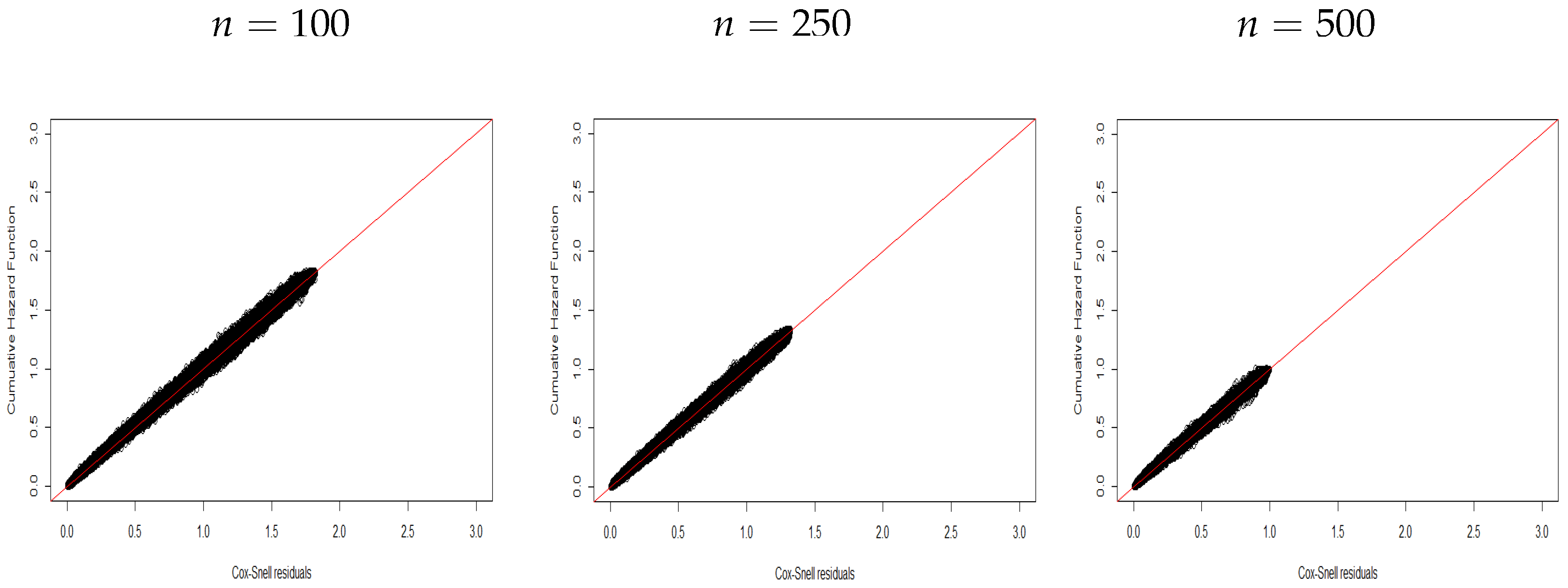
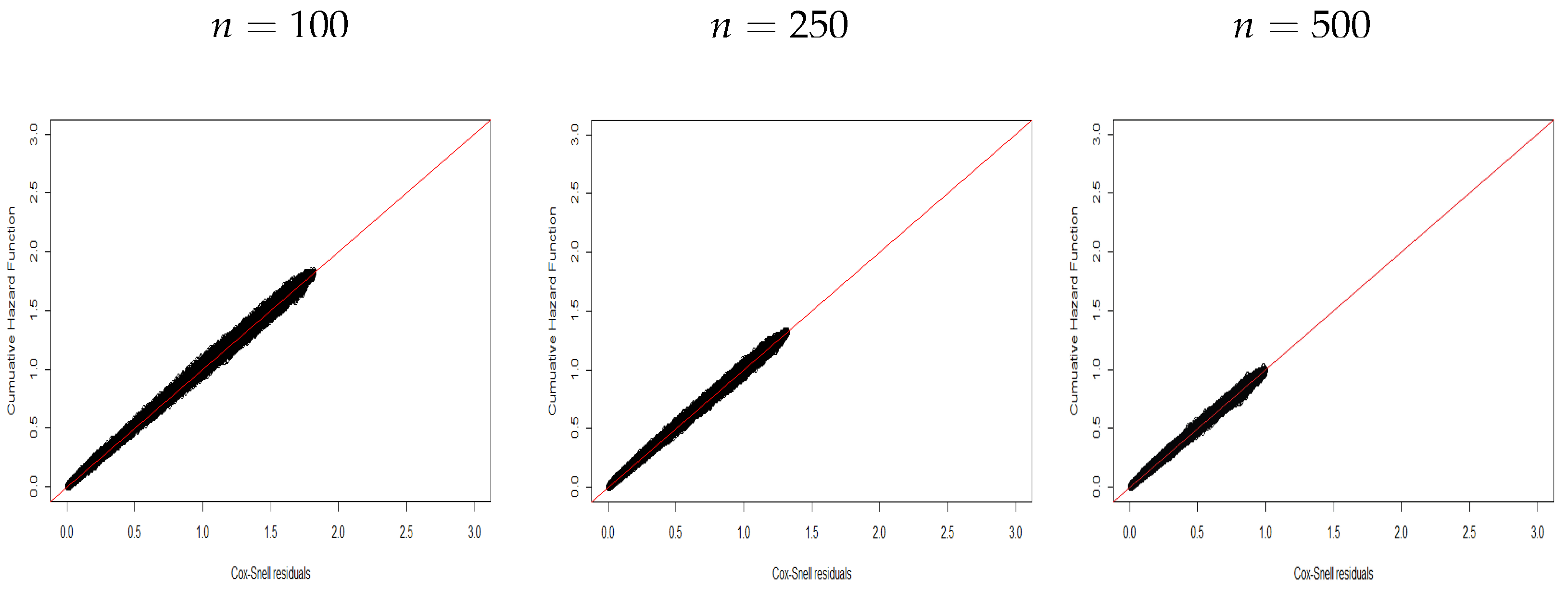
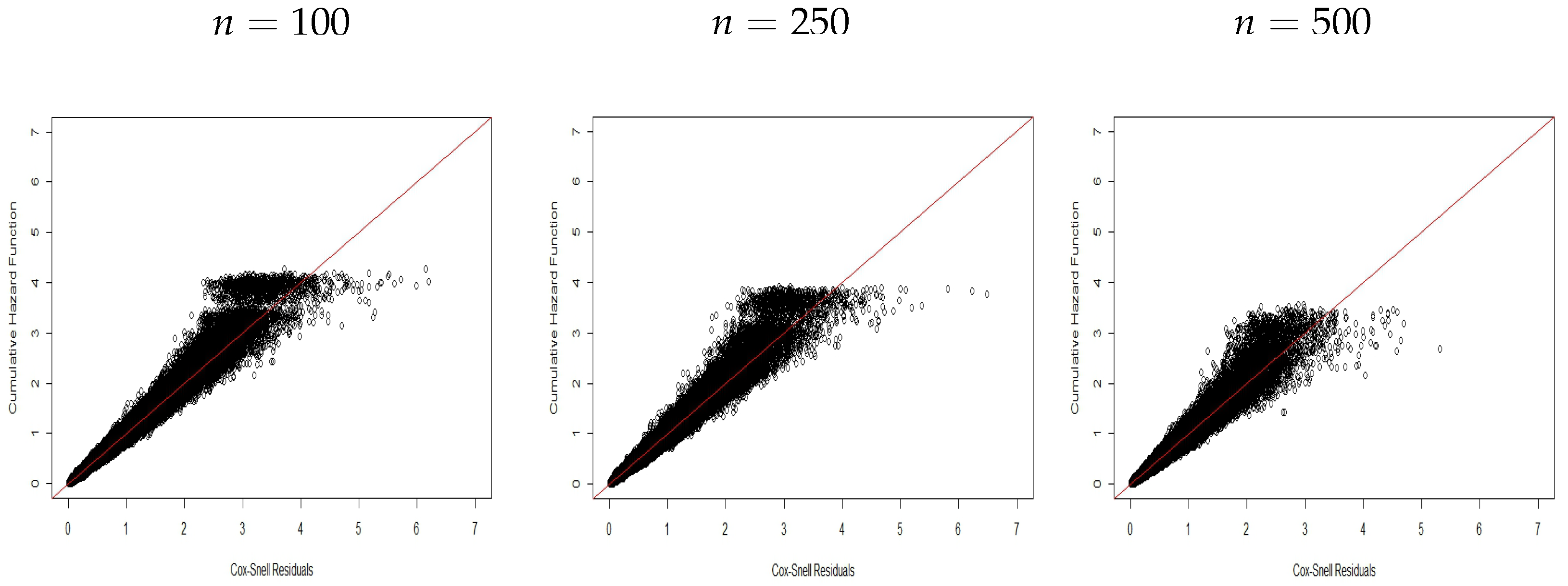
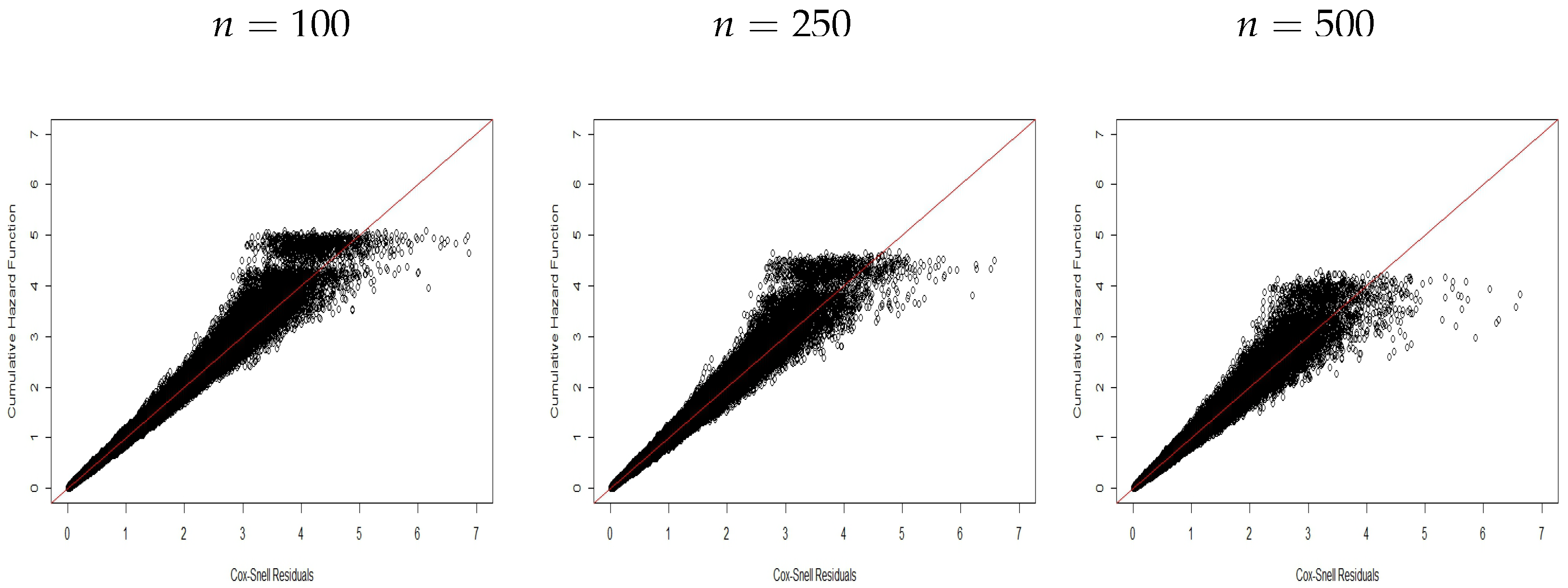
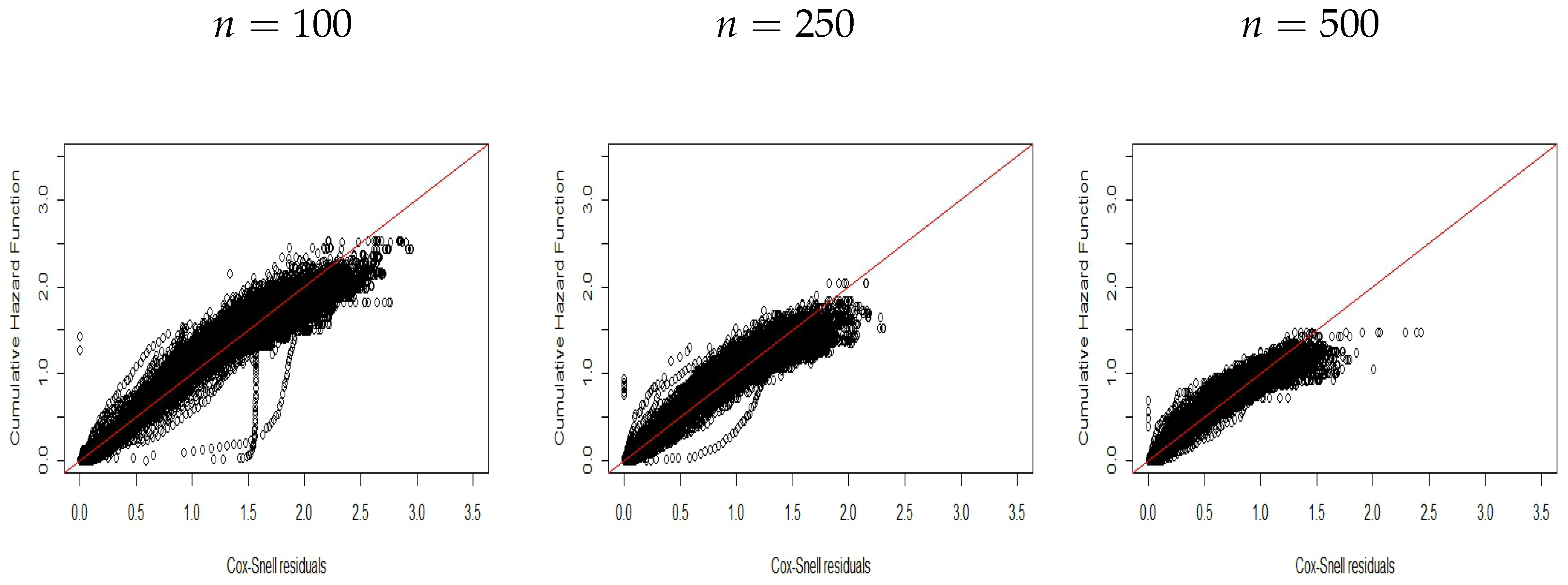
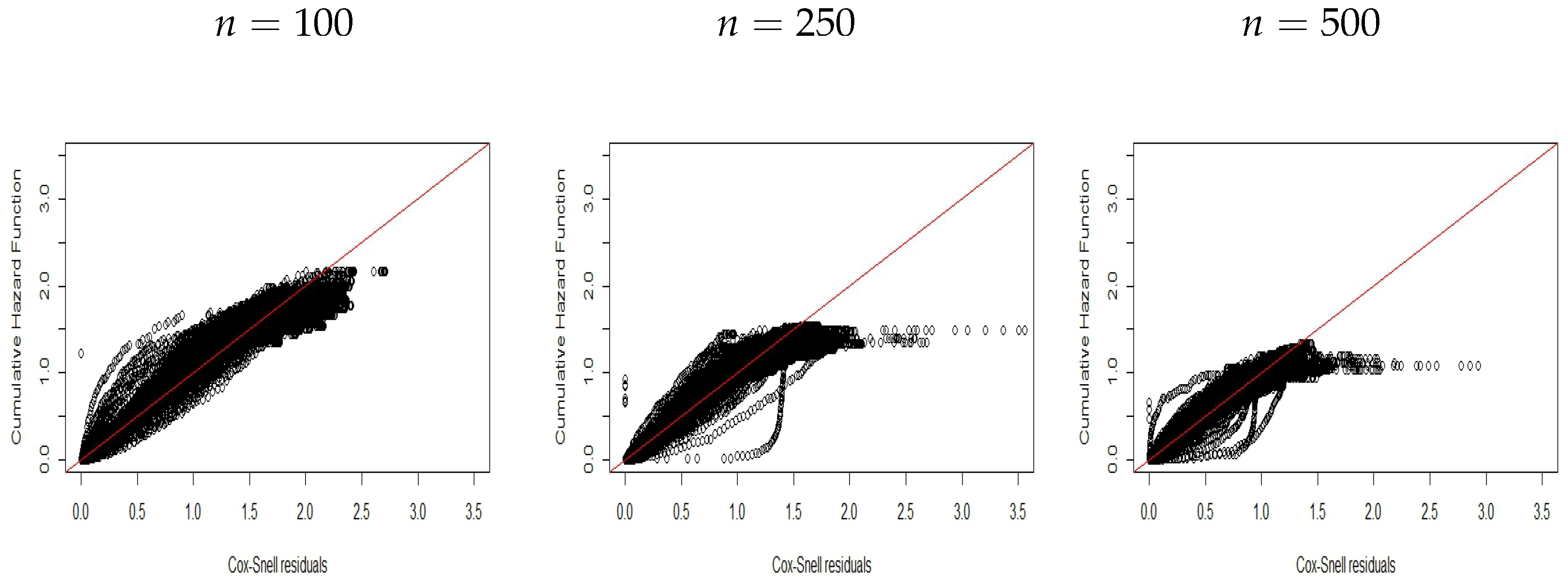
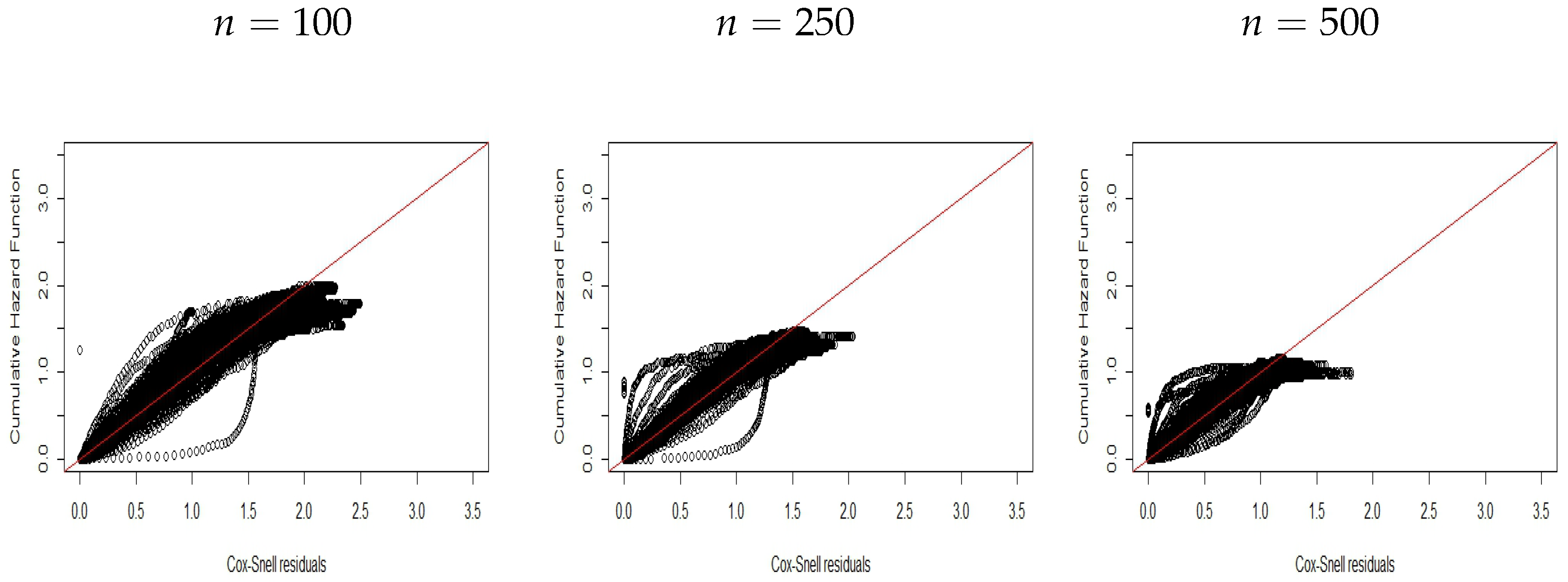
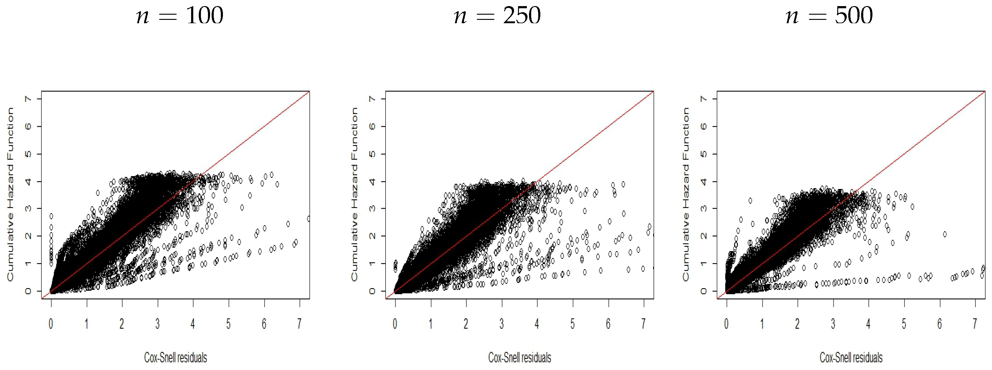
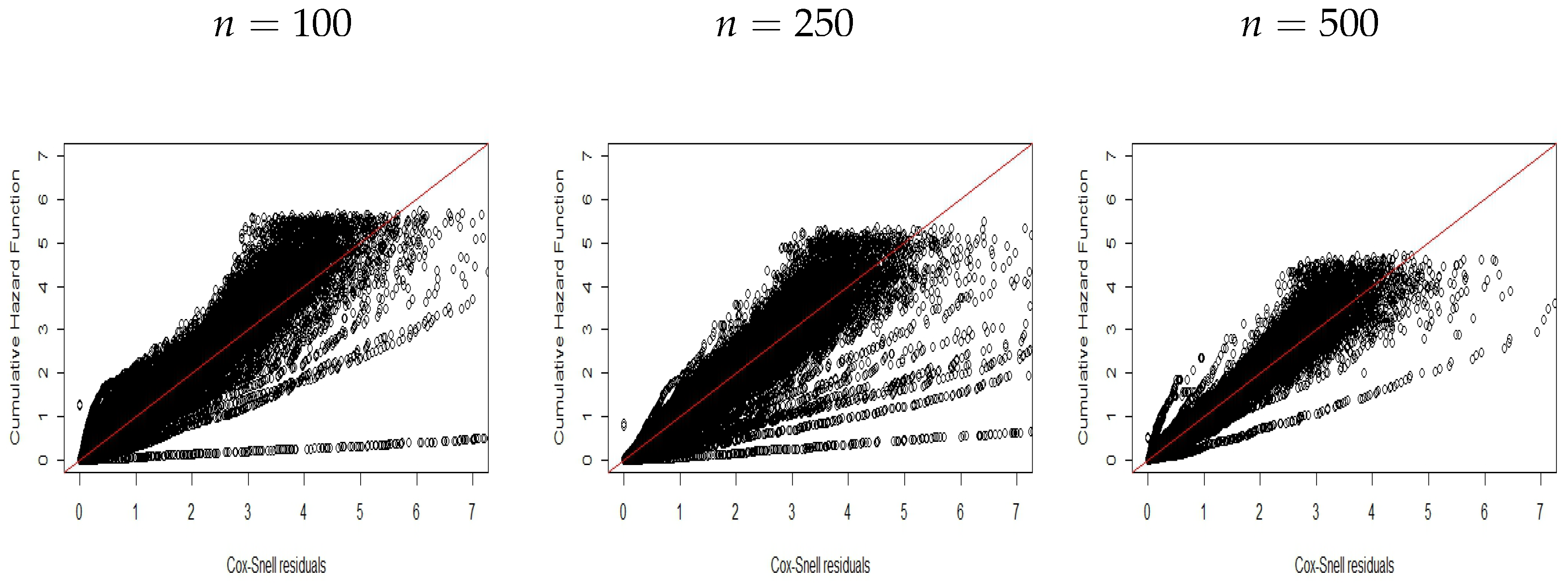
The plots below support the model assumptions. Each plot in Figure 1, Figure 2, Figure 3, Figure 4, Figure 5, Figure 6, Figure 7, Figure 8, Figure 9, Figure 10, Figure 11 and Figure 12 was prepared from 1000 replicates (under each scenario: A 1 , A 2 , B 1 , and B 2 ) based on the fact that the residuals of the replicates behave like a censored sample from an exponential distribution in the interval [ 0 , θ ) for susceptible individuals. Thus, we can use the plot of the CHF H ^ 0 ( r C S i ) = log ( S ^ 0 ( r C S i ) ) versus the ordered estimated residuals r C S i , where S ^ 0 ( r C S i ) is the Kaplan–Meier (KM) survival function. Then, the expected behavior for a corrected model fit to the data follows if these plots are close to a straight line with unity slope [27].
Figure 1, Figure 2 and Figure 3 display plots of the CHF versus the ordered Cox–Snell residuals for the new model without covariates (scenario A 1 ). So, we can conclude the following:
  • The proposed residuals have a linear behavior with unity slope.
  • The linear behavior of the residuals becomes more evident when the sample size increases.
The Cox–Snell residuals for the proposed regression with covariates (scenario A 2 ) are displayed in Figure 4, Figure 5 and Figure 6. It can be noted, due to the presence of covariates, that the expected behavior has a dispersion around the first bisector line, which is a little greater if compared to the cases without covariates. However, this preserves the pattern of a linear behavior around this line, thus evidencing the capacity of the proposed residuals to select the model that best describes the current data.

3.2. Misspecification (Scenario B)

We adopted the proposed residuals to select a model that fits well to the generated data sets by adding simulation results for scenarios B 1 and B 2 .
Figure 7, Figure 8 and Figure 9 display the plots for scenario B 1 , without covariates, which indicate that the new residuals capture the incorrect model specification.
Thus, we can note the ability of the residuals to identify the corrected distribution to the data. Similar results are reported in Figure 10, Figure 11 and Figure 12 for scenario B 2 by generating data from the PEW promotion time model with covariates with cure fraction after fitting the log-logistic promotion time model. Again, we can note that these residuals can capture the model misspecification.
Finally, all plots show the possibility of using new Cox–Snell residuals to select different distributions and find one that is adequate to describe data with cure fraction.

4. Application to Melanoma Data

We applied the proposed methods to cutaneous melanoma data discussed in [42,43]. We emphasize that these previous papers did not conduct a residual analysis for models with cure fractions. For this data set, the response variable y i is the time that elapsed from the diagnosis to death for n = 417 patients who had cutaneous melanoma with approximately 43% of censored observations. The independent variables were as follows: x i 1 : treatment (0 = observation, 1 = interferon dose); x i 2 , age (in years); x i 3 , nodule category (1 to 4); x i 4 , sex (0 = male, 1 = female); x i 5 , p.s. (performance status patients in terms of activities: 0 = fully active, 1 = other); and x i 6 , tumor thickness (in mm).

4.1. Marginal Analysis of the Response Variable

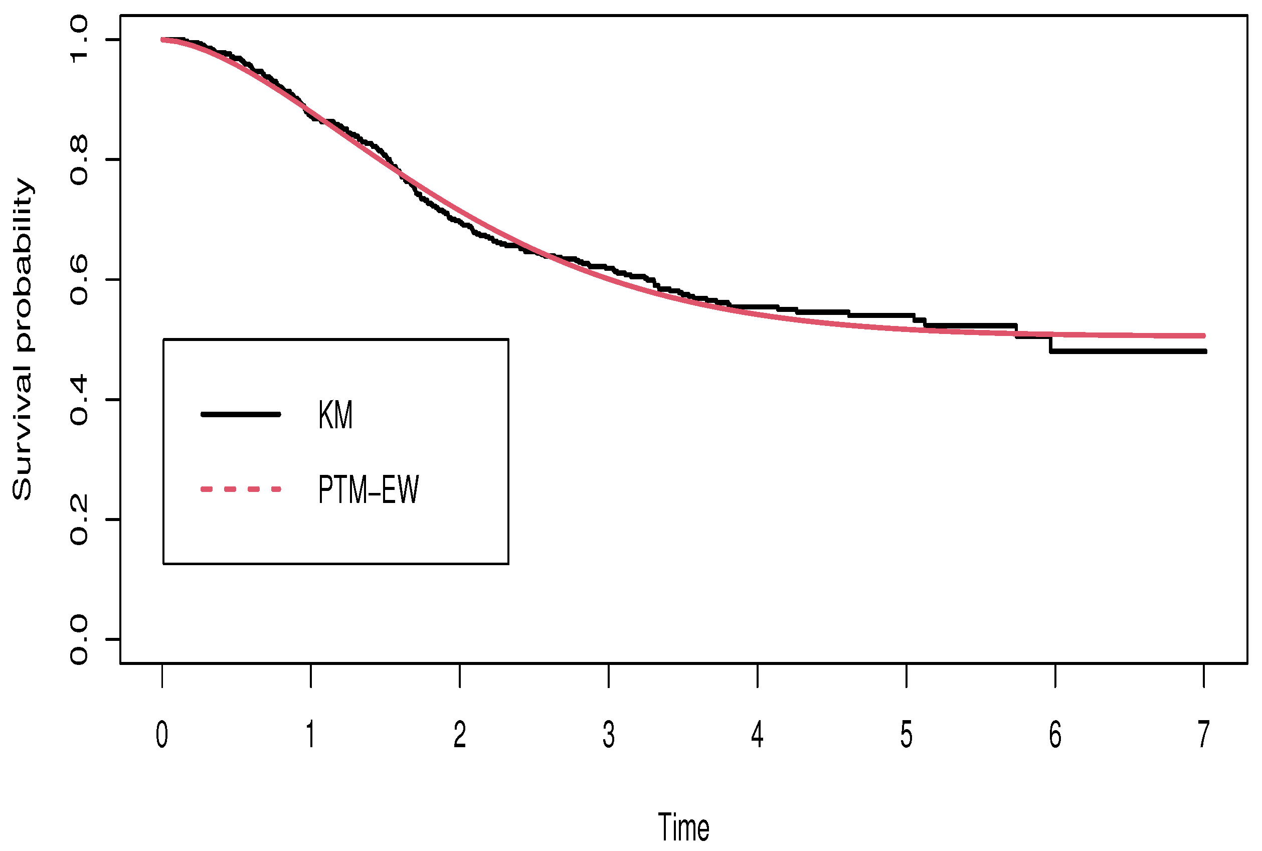
First, we analyzed the response variable. Figure 13 displays the Kaplan–Meier (KM) survival function, where an obvious cure possibility occurs after five years [44].
We consider Equation (7) to model these data marginally. Table 4 provides the MLEs and their standard errors (SEs) for the PEW model with cure fraction.
The KM and the estimated survival functions in Figure 13 reveal that the PEW model fits well to the data. The estimated proportion of cured patients is
θ ^ = e β ^ 0 = 0.6819 p ^ 0 = e θ ^ = 50.57 % ,
where the confidence interval for the proportion of cured patients is ( 44.57 % , 55.37 % ) .
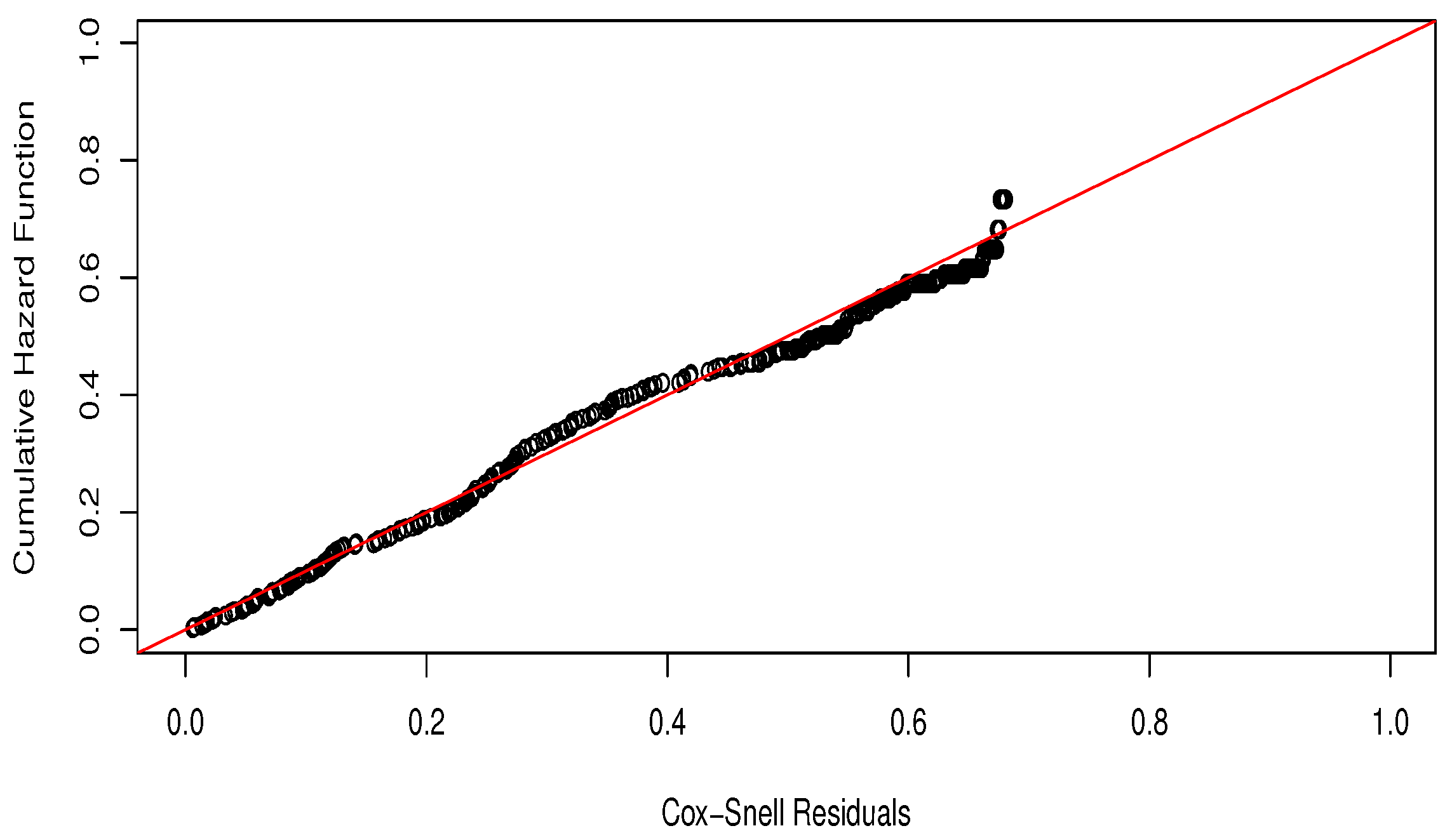
Figure 14 shows the plot of the CHF versus Cox–Snell residuals, which supports a good fit of the PEW model to these data.

4.2. The PEW-Adjusted Regression

Consider the PEW regression with cure fraction addressed in Section 2:
θ i = exp β 0 + j = 1 6 β j x i j , i = 1 , , 417 .
The MLEs and standard errors (SEs) in Table 5 were calculated using the R software [37], and they indicate that x 3 is a significant variable. Hence, the final regression is
θ i = exp ( β 0 + β 3 x i 3 ) , i = 1 , , 417 .
The MLEs and SEs in the final model are reported in Table 6. The percentage of censorship for nodule category 1 is 27%; for nodule category 2, 33%; for nodule category 3, 21%; and for category nodule 4, 19%.

4.3. Adequacy

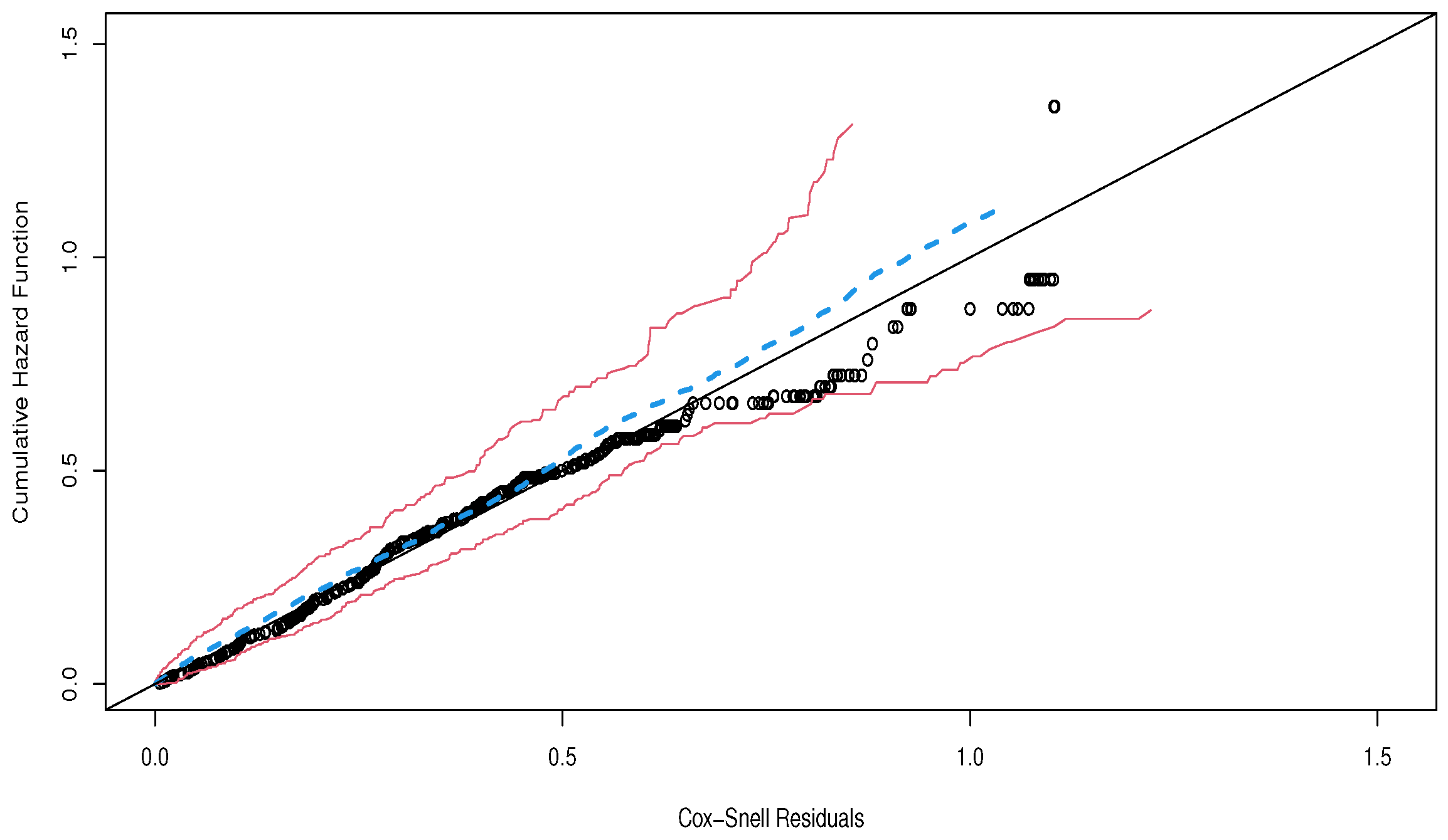
Figure 15 displays the CHF versus Cox–Snell residuals with a generated confidence envelope. The plot indicates an approximate straight line, thus showing an adequate fitted regression. Figure 16 provides the plots of the empirical and estimated survival functions for the four nodule categories, which reveal that the new regression provides a good fit to explain the time elapsed from diagnosis until death caused by cutaneous melanoma cancer.
Fitting the PEW model proved to be effective in describing the data under analysis. This model exhibits results comparable to those reported in [45], which applied the COM-Poisson Weibull model with a cure fraction among other models to cutaneous melanoma data. The findings of our study show a striking similarity with these previous results. Similarly, ref. [46] introduced the Negative Binomial Generalized Gamma model with cure rate to explain the incidence of cutaneous melanoma. The results obtained in [46] and others also support the conclusions obtained from our adjusted PEW model.
However, although both studies mentioned corroborate the applicability of the PEW model in similar contexts, there is still a significant gap in the literature in terms of evaluating the adjusted model through residual analysis. There are no established methods that offer an accurate distribution of waste and are simultaneously easy to implement. Therefore, we emphasize that the residuals developed in our study offer a considerable advantage in evaluating fitted models. In calculating these residuals, it is possible to carry out a more precise and detailed analysis of the adjusted model, thus improving the reliability of the statistical inferences made.

5. Conclusions

Several simulations performed in this study indicated that the Cox–Snell residuals for the Poisson-exponentiated Weibull (PEW) regression showed a linear behavior around the first bisector, thus evidencing the capacity of these residuals to select the best model for the current data. The proposed methods of residuals and envelopes for survival models with cured fraction can be employed to assess the suitability of the proposed models for the data. This utilization can be similar to what is performed in the case of the normal linear model, evaluating the quality of model fit by comparing the residuals with a reference probability distribution and simulated envelopes. In this way, the contributions of this study can be understood in the common context of model fitting and checking the adequacy of regression models. Similarly, future research may be conducted to study these residuals in other models with cure fraction. Further, note that these residuals for the PEW regression model with cure fraction can be easily extended to other regression sub-models (Weibull, log-logistic, exponentiated exponential, log-normal, and Rayleigh, among others) since the EW distribution has some special cases widely used in survival analysis. Finally, other works can be developed to extend the Cox–Snell residuals for several regression models with cure fractions in the literature, such as the COM-Poisson cure rate survival models, destructive negative binomial cure rate models, Conway–Maxwell–Poisson generalized gamma regression models, a power series beta Weibull regression model, survival models induced by discrete frailty for modeling lifetime data with long-term survivors, power series cure rate models for spatially correlated interval-censored data, and long-term bivariate survival Farlie–Gumbel–Morgenstern copula models (bivariate case), among others.

Author Contributions

All the authors contributed equally to this work. All authors have read and agreed to the published version of the manuscript.

Funding

This research received no external funding.

Institutional Review Board Statement

Not applicable.

Informed Consent Statement

Not applicable.

Data Availability Statement

Stated in the text.

Acknowledgments

This work was supported by CNPq and CAPES, Brazil.

Conflicts of Interest

The authors declare no conflicts of interest.

Appendix A. Proof for Basal Distribution of Cox–Snell Residuals

Here, we prove that the reference distribution is of a mixed type with a censored continuous exponential part and a degenerate discrete part at θ . Letting w e θ , 1 and V = min { Z 1 , , Z M } , we have
P S pop ( T ) w = P exp { θ [ F ( T ) ] } w = P T > F 1 log ( w ) θ = P T > F 1 log ( w ) θ | M = 0 P θ ( M = 0 ) = p θ ( 0 ) + m = 1 P V > F 1 log ( w ) θ | M = m p θ ( m ) = p θ ( 0 ) + m = 1 1 F F 1 log ( w ) θ m p θ ( m ) .
So, we can write
P S pop ( T ) w = m = 0 1 + log ( w ) θ m p θ ( m ) .
On the other hand, since M P o i s s o n ( θ ) , the generating function (gf) of M can be expressed as
M M ( t ) = m = 0 exp ( t m ) p θ ( m ) = exp θ exp ( t ) 1 .
Further, we obtain from the previous expression
E a M = M M [ log ( a ) ] = exp θ ( a 1 ) .
Using these results in Equation (A1), we have
P S pop ( T ) x = x .
The Cox–Snell residuals follow an F ( T ) distribution, since H ( T , θ ) = log S pop ( T ) . For v R , we can write
P log [ S pop ( T ) ] > v = P log [ S pop ( T ) ] v = P S pop ( T ) e v = 0 , e v < e θ , e v , e θ e v < 1 , 1 , e v 1 .
Finally,
P log [ S pop ( T ) ] > v = 1 , v 0 , e v , 0 < v θ , 0 , v > θ .

References

  1. Berkson, J.; Gage, R.P. Survival curve for cancer patients following treatment. J. Am. Stat. Assoc. 1952, 47, 501–515. [Google Scholar] [CrossRef]
  2. Boag, J.W. The presentation and analysis of the results of radiotherapy. Br. J. Radiol. 1948, 21, 128–138. [Google Scholar] [CrossRef] [PubMed]
  3. Boag, J.W. Maximum likelihood estimates of the proportion of patients cured by cancer therapy. J. R. Stat. Soc. Ser. B (Methodol.) 1949, 11, 15–53. [Google Scholar] [CrossRef]
  4. Tsodikov, A.D.; Yakovlev, A.Y.; Asselain, B. Stochastic Models of Tumor Latency and Their Biostatistical Applications; World Scientific: Singapore, 1996; Volume 1. [Google Scholar]
  5. Mudholkar, G.S.; Srivastava, D.K. Exponentiated Weibull family for analyzing bathtub failure-rate data. IEEE Trans. Reliab. 1993, 42, 299–302. [Google Scholar] [CrossRef]
  6. Nadarajah, S.; Cordeiro, G.M.; Ortega, E.M. The exponentiated Weibull distribution: A survey. Stat. Pap. 2013, 54, 839–877. [Google Scholar] [CrossRef]
  7. Mudholkar, G.S.; Hutson, A.D. The exponentiated Weibull family: Some properties and a flood data application. Commun. Stat. Methods 1996, 25, 3059–3083. [Google Scholar] [CrossRef]
  8. Khan, S.A. Exponentiated Weibull regression for time-to-event data. Lifetime Data Anal. 2018, 24, 328–354. [Google Scholar] [CrossRef] [PubMed]
  9. Yoosefi, M.; Baghestani, A.R.; Khadembashi, N.; Pourhoseingholi, M.A.; Akbarzadeh Baghban, A.; Khosrovirad, A. Survival analysis of colorectal cancer patients using exponentiated Weibull distribution. Int. J. Cancer Manag. 2018, 11, e8686. [Google Scholar] [CrossRef]
  10. Castro, M.d.; Cancho, V.G.; Rodrigues, J. A note on a unified approach for cure rate models. Braz. J. Probab. Stat. 2010, 24, 100–103. [Google Scholar] [CrossRef]
  11. Rodrigues, J.; de Castro, M.; Balakrishnan, N.; Cancho, V.G. Destructive weighted Poisson cure rate models. Lifetime Data Anal. 2011, 17, 333–346. [Google Scholar] [CrossRef]
  12. Cancho, V.G.; Louzada, F.; Barriga, G.D. The geometric Birnbaum–Saunders regression model with cure rate. J. Stat. Plan. Inference 2012, 142, 993–1000. [Google Scholar] [CrossRef]
  13. Ortega, E.M.; Cordeiro, G.M.; Kattan, M.W. The log-beta Weibull regression model with application to predict recurrence of prostate cancer. Stat. Pap. 2013, 54, 113–132. [Google Scholar] [CrossRef]
  14. Ortega, E.M.; Cordeiro, G.M.; Campelo, A.K.; Kattan, M.W.; Cancho, V.G. A power series beta Weibull regression model for predicting breast carcinoma. Stat. Med. 2015, 34, 1366–1388. [Google Scholar] [CrossRef] [PubMed]
  15. Ramires, T.G.; Hens, N.; Cordeiro, G.M.; Ortega, E.M. Estimating nonlinear effects in the presence of cure fraction using a semi-parametric regression model. Comput. Stat. 2018, 33, 709–730. [Google Scholar] [CrossRef]
  16. Pescim, R.R.; Ortega, E.M.; Suzuki, A.K.; Cancho, V.G.; Cordeiro, G.M. A new destructive Poisson odd log-logistic generalized half-normal cure rate model. Commun. Stat. Theory Methods 2019, 48, 2113–2128. [Google Scholar] [CrossRef]
  17. Cancho, V.G.; Macera, M.A.; Suzuki, A.K.; Louzada, F.; Zavaleta, K.E. A new long-term survival model with dispersion induced by discrete frailty. Lifetime Data Anal. 2020, 26, 221–244. [Google Scholar] [CrossRef] [PubMed]
  18. Silva, G.O.; Cordeiro, G.M.; Ortega, E.M. Surviving and non surviving fraction regression models based on the beta modified Weibull distribution. Model Assist. Stat. Appl. 2020, 15, 111–126. [Google Scholar] [CrossRef]
  19. Cancho, V.G.; Barriga, G.D.; Cordeiro, G.M.; Ortega, E.M.; Suzuki, A.K. Bayesian survival model induced by frailty for lifetime with long-term survivors. Stat. Neerl. 2021, 75, 299–323. [Google Scholar] [CrossRef]
  20. Sy, J.P.; Taylor, J.M. Estimation in a Cox proportional hazards cure model. Biometrics 2000, 56, 227–236. [Google Scholar] [CrossRef]
  21. Balakrishnan, N.; Pal, S. EM algorithm-based likelihood estimation for some cure rate models. J. Stat. Theory Pract. 2012, 6, 698–724. [Google Scholar] [CrossRef]
  22. Balakrishnan, N.; Pal, S. Lognormal lifetimes and likelihood-based inference for flexible cure rate models based on COM-Poisson family. Comput. Stat. Data Anal. 2013, 67, 41–67. [Google Scholar] [CrossRef]
  23. Balakrishnan, N.; Pal, S. An EM algorithm for the estimation of parameters of a flexible cure rate model with generalized gamma lifetime and model discrimination using likelihood-and information-based methods. Comput. Stat. 2015, 30, 151–189. [Google Scholar] [CrossRef]
  24. Pal, S.; Balakrishnan, N. Likelihood inference for the destructive exponentially weighted Poisson cure rate model with Weibull lifetime and an application to melanoma data. Comput. Stat. 2017, 32, 429–449. [Google Scholar] [CrossRef]
  25. Pal, S.; Barui, S.; Davies, K.; Mishra, N. A stochastic version of the EM algorithm for mixture cure model with exponentiated Weibull family of lifetimes. J. Stat. Theory Pract. 2022, 16, 48. [Google Scholar] [CrossRef]
  26. Wileyto, E.P.; Li, Y.; Chen, J.; Heitjan, D.F. Assessing the fit of parametric cure models. Biostatistics 2013, 14, 340–350. [Google Scholar] [CrossRef] [PubMed]
  27. Scolas, S.; Legrand, C.; Oulhaj, A.; El Ghouch, A. Diagnostic checks in mixture cure models with interval-censoring. Stat. Methods Med Res. 2018, 27, 2114–2131. [Google Scholar] [CrossRef] [PubMed]
  28. Peng, Y.; Taylor, J.M. Residual-based model diagnosis methods for mixture cure models. Biometrics 2017, 73, 495–505. [Google Scholar] [CrossRef] [PubMed]
  29. Yakovlev, A.Y.; Asselain, B.; Bardou, V.; Fourquet, A.; Hoang, T.; Rochefediere, A.; Tsodikov, A. A simple stochastic model of tumor recurrence and its application to data on premenopausal breast cancer. Biom. Anal. Donnees Spatio Temporelles 1993, 12, 66–82. [Google Scholar]
  30. Tsodikov, A.D.; Asselain, B.; Fourque, A.; Hoang, T.; Yakovlev, A.Y. Discrete strategies of cancer post-treatment surveillance. Estimation and optimization problems. Biometrics 1995, 51, 437–447. [Google Scholar] [CrossRef]
  31. Yin, G.; Ibrahim, J.G. Cure rate models: A unified approach. Can. J. Stat. 2005, 33, 559–570. [Google Scholar] [CrossRef]
  32. Tsodikov, A.; Ibrahim, J.; Yakovlev, A. Estimating cure rates from survival data: An alternative to two-component mixture models. J. Am. Stat. Assoc. 2003, 98, 1063–1078. [Google Scholar] [CrossRef] [PubMed]
  33. Rodrigues, J.; Cancho, V.G.; de Castro, M.; Louzada-Neto, F. On the unification of long-term survival models. Stat. Probab. Lett. 2009, 79, 753–759. [Google Scholar] [CrossRef]
  34. Cancho, V.G.; Ortega, E.M.; Bolfarine, H. The log-exponentiated-Weibull regression models with cure rate: Local influence and residual analysis. J. Data Sci. 2009, 7, 433–458. [Google Scholar] [CrossRef]
  35. Liu, D.C.; Nocedal, J. On the limited memory BFGS method for large scale optimization. Math. Program. 1989, 45, 503–528. [Google Scholar] [CrossRef]
  36. Henningsen, A.; Toomet, O. maxLik: A package for maximum likelihood estimation in R. Comput. Stat. 2011, 26, 443–458. [Google Scholar] [CrossRef]
  37. R Core Team. R: A Language and Environment for Statistical Computing; R Foundation for Statistical Computing: Vienna, Austria, 2020. [Google Scholar]
  38. Lawless, J.F. Statistical Models and Methods for Lifetime Data; John Wiley & Sons: Hoboken, NJ, USA, 2003; Volume 362. [Google Scholar]
  39. Cox, D.R.; Snell, E.J. A general definition of residuals. J. R. Stat. Soc. Ser. B (Methodol.) 1968, 30, 248–265. [Google Scholar] [CrossRef]
  40. Atkinson, A.C. Plots, Transformations and Regression: An Introduction to Graphical Methods of Diagnostic Regression Analysis; Technical Report; Oxford University Press: Oxford, UK, 1985. [Google Scholar]
  41. Kaplan, E.L.; Meier, P. Nonparametric estimation from incomplete observations. J. Am. Stat. Assoc. 1958, 53, 457–481. [Google Scholar] [CrossRef]
  42. Ibrahim, J.G.; Chen, M.H.; Sinha, D. Bayesian Survival Analysis; Springer Science & Business Media: Berlin/Heidelberg, Germany, 2001. [Google Scholar]
  43. Mizoi, M.F.; Bolfarine, H.; Pedroso-De-Lima, A.C. Cure rate model with measurement error. Commun. Stat. Comput. 2007, 36, 185–196. [Google Scholar] [CrossRef]
  44. Maller, R.A.; Zhou, X. Survival Analysis with Long-Term Survivors; Wiley: New York, NY, USA, 1996. [Google Scholar]
  45. Rodrigues, J.; de Castro, M.; Cancho, V.G.; Balakrishnan, N. COM–Poisson cure rate survival models and an application to a cutaneous melanoma data. J. Stat. Plan. Inference 2009, 139, 3605–3611. [Google Scholar] [CrossRef]
  46. Ortega, E.M.; Barriga, G.D.; Hashimoto, E.M.; Cancho, V.G.; Cordeiro, G.M. A New Class of Survival Regression Models with Cure Fraction. J. Data Sci. 2014, 12, 107–136. [Google Scholar] [CrossRef]
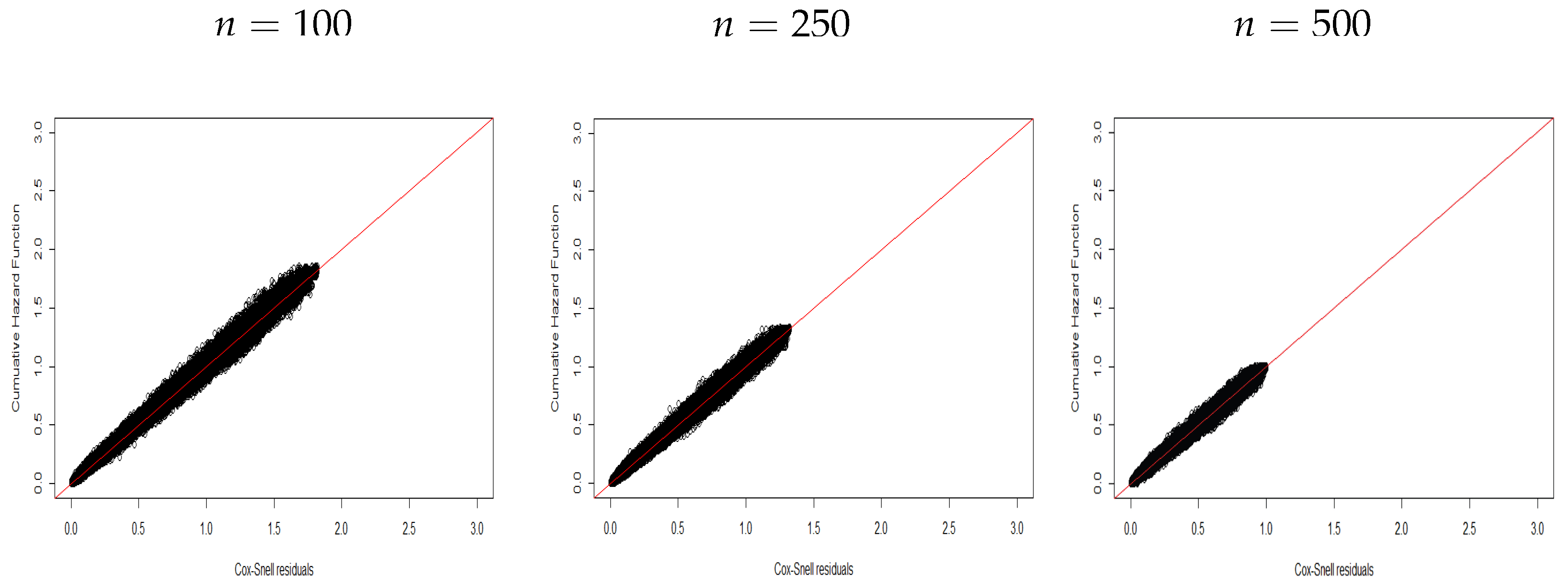
Figure 1. CHF versus residuals for Scenario A 1 .
Stats 07 00030 g001
Figure 2. CHF versus residuals for Scenario A 1 .
Stats 07 00030 g002
Figure 3. CHF versus residuals for Scenario A 1 .
Stats 07 00030 g003
Figure 4. CHF versus residuals for Scenario A 2 .
Stats 07 00030 g004
Figure 5. CHF versus residuals for Scenario A 2 .
Stats 07 00030 g005
Figure 6. CHF versus residuals for Scenario A 2 .
Stats 07 00030 g006
Figure 7. CHF versus residuals for Scenario B 1 .
Stats 07 00030 g007
Figure 8. CHF versus residuals for Scenario B 1 .
Stats 07 00030 g008
Figure 9. CHF versus residuals for Scenario B 1 .
Stats 07 00030 g009
Figure 10. CHF versus residuals for Scenario B 2 .
Stats 07 00030 g010
Figure 11. CHF versus residuals for Scenario B 2 .
Stats 07 00030 g011
Figure 12. CHF versus residuals for Scenario B 2 .
Stats 07 00030 g012
Figure 13. The KM and estimated survival function from the PEW model with cure fraction.
Stats 07 00030 g013
Figure 14. The KM survival function.
Stats 07 00030 g014
Figure 15. Cox–Snell residuals with envelope for the fitted PEW regression.
Stats 07 00030 g015
Figure 16. Estimatedsurvival functions from the PEW regression and empirical survivals for the nodule categories in the melanoma data.
Stats 07 00030 g016
Table 1. Percentages of censoring and cure fraction for the simulations.
Level of CensoringPercentage of CensoringPercentage of Cure Fraction
Light20%10%
Moderate30%20%
High40%30%
Table 2. Fixed values of β 0 and u for generating data without covariates.
Level of
Censoring
β 0 u
Light0.503.45
Moderate0.182.05
High−0.101.42
Table 3. Fixed parameters values and u and β for generating data with covariates.
Level of
Censoring
β 0 β 1 β 2 β 3 u
Light0.251.201.801.002.70
Moderate0.501.351.20−0.901.40
High−0.351.001.20−0.901.10
Table 4. Findings from the fitted PEW model with cure fraction.
ParameterEstimateSE
β 0 −0.38280.0820
α 1.87810.3646
γ 0.87340.2474
λ 0.37690.0562
Table 5. Findings from the fitted new regression.
ParameterEstimateSEp-Value
β 0 −0.38610.35120.2715
β 1 0.01920.14410.8937
β 2 −0.00890.00560.1096
β 3 0.22040.06880.0013
β 4 −0.10420.14910.4848
β 5 0.06250.21440.7706
β 6 −0.00150.02260.9464
α 1.87840.3684-
γ 0.7760.2458-
λ 0.36780.0544-
Table 6. Findings from the final fitted model.
ParameterEstimateSEp-Value
β 0 −0.99730.1889<0.001
β 3 0.27730.0672<0.001
α 1.74890.4416-
γ 0.99640.3671-
λ 0.38430.0713-
Disclaimer/Publisher’s Note: The statements, opinions and data contained in all publications are solely those of the individual author(s) and contributor(s) and not of MDPI and/or the editor(s). MDPI and/or the editor(s) disclaim responsibility for any injury to people or property resulting from any ideas, methods, instructions or products referred to in the content.