Article

Asymptotic Relative Efficiency of Parametric and Nonparametric Survival Estimators

BioPharma Early Biometrics and Statistical Innovation, Data Science & AI, BioPharmaceuticals R&D, AstraZeneca, 43183 Gothenburg, Sweden
Stats 2023, 6(4), 1147-1159; https://doi.org/10.3390/stats6040072
Submission received: 13 September 2023 / Revised: 20 October 2023 / Accepted: 21 October 2023 / Published: 25 October 2023
(This article belongs to the Section Survival Analysis)

Abstract

:
The dominance of non- and semi-parametric methods in survival analysis is not without criticism. Several studies have highlighted the decrease in efficiency compared to parametric methods. We revisit the problem of Asymptotic Relative Efficiency ( A R E ) of the Kaplan–Meier survival estimator compared to parametric survival estimators. We begin by generalizing Miller’s approach and presenting a formula that enables the estimation (numerical or exact) of A R E for various survival distributions and types of censoring. We examine the effect of follow-up time and censoring on A R E . The article concludes with a discussion about the reasons behind the lower and time-dependent A R E of the Kaplan–Meier survival estimator.

1. Introduction

In medical statistics, survival analysis is often performed using the nonparametric Kaplan–Meier estimator [1] together with the semiparametric Proportional Hazards Model by Cox [2]. Although the theory of parametric estimators of survival is well-developed [3], their application has been limited in biomedical research. Miller [4] was one of the first to criticize this practice and highlight the loss of efficiency compared to parametric methods. Miller’s work was continued by Klein and Moeschberger [5] and Aranda-Ordaz [6] and was partly rebutted by Meier and collaborators [7] and recently touched upon by Jullum and Hjort [8]. Cheng and Lin [9] proposed a new maximum likelihood estimator under the competing risks model with proportional hazards and assessed its efficacy against the Kaplan–Meier estimator.
In this paper, we revisit the problem of the Asymptotic Relative Efficiency ( A R E ) of the Kaplan–Meier estimator compared to parametric estimators of survival. We begin by extending Miller’s method for calculating the Asymptotic Relative Efficiency ( A R E ) and present a formula that enables the estimation (numerical or exact) of A R E for various survival and censoring distributions, as well as different censoring types. We examine how censoring and the type of censoring affect A R E and discuss the reasons behind the lower and time-dependent A R E of the Kaplan–Meier estimator compared to parametric estimators of survival.

2. Notation and Estimators

We assume that the survival times for an event of interest, X 1 , , X n , are distributed independently and identically according to the distribution function F ( x ) and the survival function S ( x ) = 1 F ( x ) . We do not always have complete information for all subjects due to loss to follow-up or insufficient follow-up time. The times to censoring are denoted by C 1 , C n , and are assumed to be independent and identical, and survival function G ¯ ( c ) = 1 G ( c ) . Further censoring occurs when the study period ends at the pre-determined time τ ; all remaining subjects at risk are censored. Thus, the actual observed time for the subject j is T j = min X j , C j τ . We assume independence between failure and censoring time. We define δ j = I X j C j τ as an event indicator, taking values 1 if an event is recorded prior to censoring, otherwise 0. We consider two competing estimators for the survival function S ( t ) , the nonparametric Kaplan–Meier estimator, and the parametric maximum likelihood estimator, noted hereafter with the subscripts k m and m l . Their respective variances will be noted as v k m and v m l . In addition, we define N ( t ) = j n I ( T j t , δ j = 1 ) , the process that counts the number of events in ( 0 , t ] and R ( t ) = j n I ( T j > t ) the number at risk at time t. Although the index is not used to simplify notation through the whole of the text, we generally deal with sequences of estimators indexed by the sample size n.

2.1. The Kaplan–Meier Estimator

The naïve nonparametric survival function estimator S ( t ) = n 1 N ( t ) is only feasible when there is no censoring in the data, i.e., P ( X C ) = 1 . In this case, the survival at t is a binomial probability with variance n 1 S ( t ) ( 1 S ( t ) ) .
The nonparametric product limit or Kaplan–Meier estimator [1] that can incorporate censored data is given by
S k m t = T i t 1 δ i R T i ,
where T i is the ordered sequence of observed event times and t is the absolute time. The Kaplan–Meier is asymptotically unbiased and has as a limiting distribution
n S ^ k m ( t ) S ( t ) D N ( 0 , v k m ) ,
with asymptotic variance
v k m ( t ) = 1 n 1 F ( t ) 2 0 t f ( u ) 1 F ( u ) 2 1 G ( u ) d t .
This requires knowledge of the survival and censoring distribution, thus is not applicable in real-life situations and its nonparametric variant, the Greenwood estimator, is used:
v k m ( t ) = S k m 2 t T i t δ i R T i R T i δ i .
There are alternatives to the Greenwood variance estimator, but as Klein [10] concluded, the variance-bias trade-off favours the Greenwood estimator.

The Parametric Survival Estimator

Next, we establish the notation for the maximum likelihood estimators. The parametric survival function is given by S ^ m l ( t , θ ^ ) , where θ ^ = arg max θ l n ( θ ) with l n ( θ ) = i = 1 n log f ( X i , θ ) being the log-likelihood function of the data
l ( θ T i , δ i ) = i = 1 n f ( T i ) G ¯ ( T i ) δ i ( 1 F ( T i ) ) g ( T i ) 1 δ i .
As the censoring distribution G does not depend on θ , censoring does not contribute to the estimation of θ m l and it is factored out during maximization of the likelihood. On the other hand, the variance and Fisher information of θ m l does account for censoring [11,12], with
J T ( θ ) = 0 θ log f 2 f G ¯ d x = J X ( θ ) P ( X < C ) ,
with the superscript T indicating that calculation refers to the observed follow-up time, while the superscript X is the possibly unobserved survival times. Here, P ( X < C ) = 0 F ( u ) g ( u ) d u [13]. In addition we define the score function U ( t , θ ) as the first derivative of log f ( X i , θ ) with regard to θ .
Under mild regularity conditions, the maximum likelihood estimator is consistent and converges in probability θ ^ m l P θ as the sample size n and is asymptotically normally distributed,
n S ^ m l ( θ ^ ; t ) S ( θ 0 ; t ) D N ( 0 , v m l ) ,
with variance v m l
v m l ( t ) = 1 n S m l ( t , θ ) θ t J 1 S m l ( t , θ ) θ ,
where J is the Fisher information matrix.

3. Asymptotic Relative Efficiency

For the statistic of interest S ( t ) and for consistent estimators S k m ( t ) and S m l ( t ) , the Asymptotic Relative Efficiency is given by
A R E ( S k m ( t ) , S m l ( t ) , F ) = v m l ( t ) v k m ( t ) .
From the Cramér–Rao theorem, we know that A R E ( S k m S m l , F ) 1 , and A R E are the needed factor change in the sample size so that the competing estimators perform equally [14].
Theorem 1. 
Under the assumption that S k m ( t ) S ( t ) and S m l ( t ) S ( t ) as n , Equation (9) with censoring considered can be defined as
A R E ( S k m ( t ) , S m l ( t ) , F ) = S m l ( t , θ ) θ t J X ( θ ) P ( X < C ) S ( t ) ( 1 S ( t ) ) φ ( t ) 1 S m l ( t , θ ) θ .
Proof. 
The naïve nonparametric survival function estimator S ^ ( t ) = n 1 N ( t ) it is feasible only when there is no censoring in the data, i.e., P ( X C ) = 1 . In this case, the survival at t is a binomial probability with variance n 1 S ( t ) ( 1 S ( t ) ) . As information is lost due to censoring of the binomial variance being inflated by factor φ t [15], where
φ t = S t 1 S t 0 t α u S u G ¯ u d u
and n 1 S ^ t 1 S ^ t φ t is estimated by the Greenwood variance estimator. Censoring causes a loss of information with J T ( θ ) = J X ( θ ) P ( X < C ) [11,12], where P ( X < C ) = 0 F ( u ) g ( u ) d u [13]. The Delta-method variance of the maximum likelihood survival estimate, considering the proportion of censoring, is
1 n J X ( θ ) P ( X < C ) S m l ( t , θ ) θ 2 ,
while the variance of the nonparametric Kaplan–Meier estimate with variance inflation due censoring is given by
1 n S k m ( t ) ( 1 S k m ( t ) ) φ ( t ) .
By plugging these two estimators into Equation for A R E , we conclude the proof. □

4. ARE as Correlation between Estimates

Crámer [16] showed that A R E equals the square of the correlation between the competing estimates, ρ 2 , with
ρ ^ ( S k m ( t ) , S m l ( t ) ) = v c ( t ) v k m ( t ) v m l ( t ) ,
where v c = C o v ( S k m ( t ) , S m l ( t ) ) . A necessary and sufficient condition for Crámer’s A R E to equal A R E as defined in Equation (9) is that v c equals the variance of the most efficient estimator. As both S k m ( t ) and S m l ( t ) are consistent estimates of S ( t ) , then for any constant α , a linear combination of the two in the form of α S k m ( t ) ( 1 α ) S m l ( t ) is also unbiased and has variance
{ 1 α } 2 v k m ( t ) + 2 α { 1 α } v c ( t ) + α 2 v m l ( t ) .
This variance is minimum at α = 0 and the derivative at α = 0 , thus v c ( t ) = v m l ( t ) . This of course does not imply that v c ( t ) and v m l ( t ) will return equal estimates in finite samples but they have the same limit as n . The estimator for v c ( t ) is presented in the Appendix.

5. ARE for Exponential Survival and Exponential Censoring

In this section, we provide closed form solutions based on Theorem 1 for exponential survival and censoring times. Besides the existence of a closed form solution for A R E , the A R E of the exponential distribution can be considered as a lower bound to many distributions used in survival analysis such as Weibull, Gamma, or Generalized Gamma, or any other parametric extension of the exponential distribution. The addition of extra parameters to the model results in the diagonal elements of the inverse of the information matrix being always greater than the corresponding elements of the simpler model. In the following, we assume exponential survival times with hazard λ and exponential censoring times with hazard γ . The survival function for exponential survival times is S λ ( t ) = e t λ with variance V a r ( S λ ( t ) ) = t 2 ( e t λ ) 2 λ 2 n 1 . Moreover, as F is known to be an exponential distribution, the event probability for the binomial distribution is p ( t ) = e λ t . In this case, we have a closed form solution for Theorem 1,
A R E ( t ) = ( t λ ) 2 ( e λ t 1 ) P ( X < C ) φ ( t ) .
We will now consider four scenarios: (1) no censoring, (2) random censoring, (3) type I censoring with fixed censoring times, and (4) hybrid, type I, and random censoring times. For the sake of simplicity, we will denote A R E with subscripts 1, 2, 3, and 4 for each scenario.

5.1. No-Censoring

If the survival time is recorded for every study participant, then φ ( t ) = P ( x < Y ) = 1 giving
A R E 1 ( t ) = ( t λ ) 2 ( e λ t 1 ) .
In this case, the maximum efficacy of the nonparametric estimator is 64.76% and happens at t = 1.593 λ 1 , i.e., 1.6 times the mean survival time.

5.1.1. Random Censoring Times

In this scenario, the observed time for subject j is T j = min X j , C j and δ j = I X j C j . Additionally, we have
P ( X < C ) = λ λ + γ and φ t = λ λ + γ e t λ + γ 1 e t λ 1 .
Combing the above with Equation (15), the asymptotic relative efficiency is
A R E 2 ( t ) = { t ( λ + γ ) } 2 ( e t ( λ + γ ) 1 ) .
The maximum efficacy of the nonparametric estimator is observed at t = 1.593 ( λ + γ ) 1 , and as for the non-censored case, it equals 64.76%. As 1.593 ( λ + γ ) 1 1.593 ( λ ) 1 , this maximum is reached earlier, and in the beginning of the follow-up period, censoring increases the efficiency of the Kaplan–Meier estimator (Figure 1).

5.1.2. Type I or Fixed Censoring

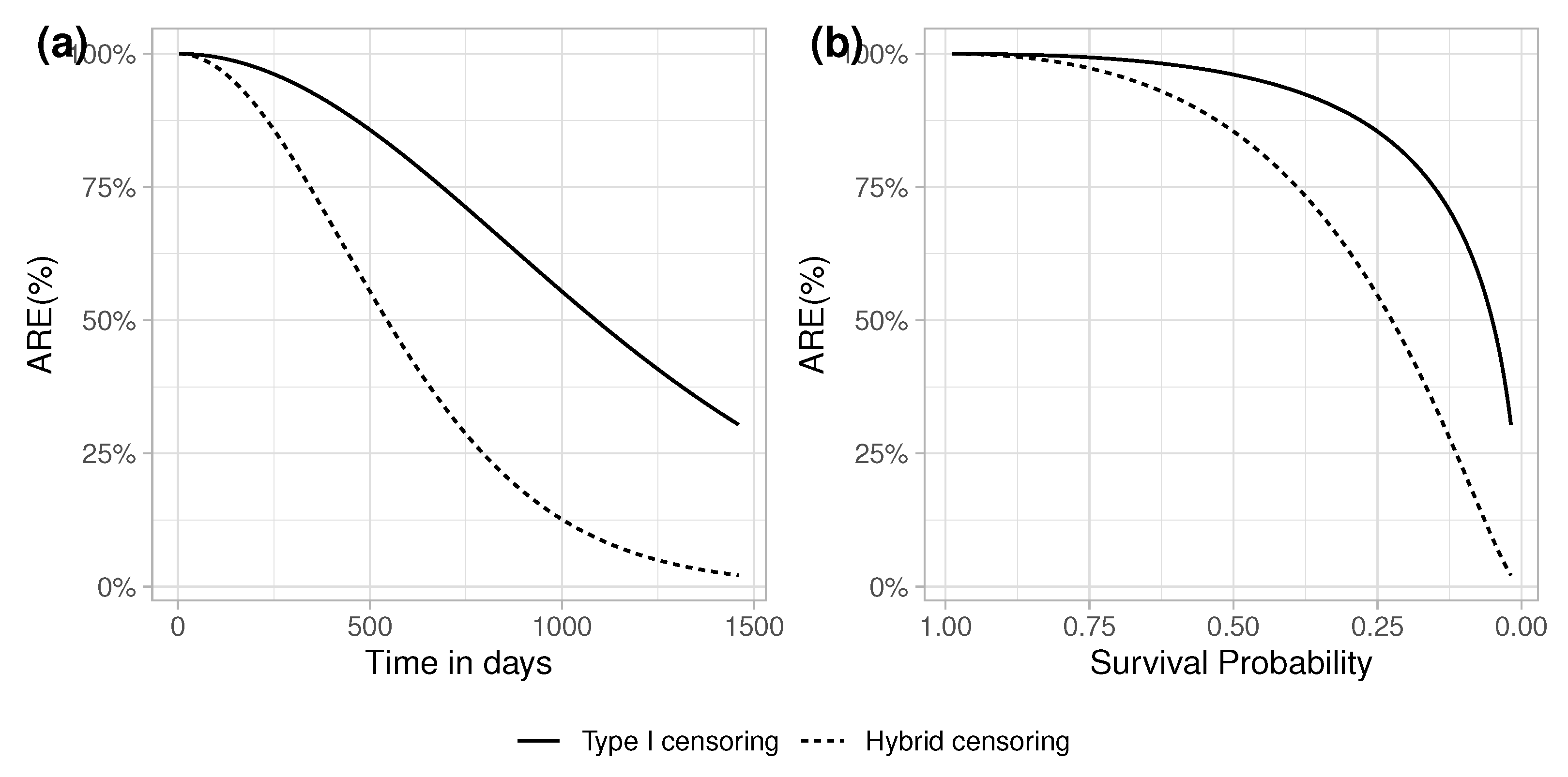
Here, the observed time for subject j is T j = min X j , τ and δ j = I X j τ . In this case, t < τ φ ( t ) = 1 and P ( X < τ ) = ( 1 e λ τ ) , resulting in
A R E 3 ( t ) = ( t λ ) 2 ( e t λ 1 ) ( 1 e λ τ ) .
As ( 1 e λ τ ) 1 , the A R E of the nonparametric variance estimator exceeds the A R E of the nonparametric variance estimator when there is no censoring and lim τ A R E 2 ( t ) = A R E 1 ( t ) .

5.1.3. Hybrid Type I and Random Censoring

Here, just as for Type I censoring, follow-up is stopped at a pre-assigned time point τ , but in addition participants might leave the study prior to τ for reasons unrelated to the studied disease. Thus, T j = min X j , C j τ . The minimum of two exponentially distributed variables with parameters λ and γ is also exponentially distributed with parameter λ + γ , thus
A R E 4 ( t ) = ( t ( λ + γ ) ) 2 ( e t ( λ + γ ) 1 ) ( 1 e ( λ + γ ) τ ) .
Type I (or fixed) censoring has no impact on the Greenwood variance estimator, but it does reduce the information available in the data for the estimation of the parametric variance with P ( X < C τ ) and improves the A R E of the Kaplan–Meier estimator up τ by P ( X < C τ ) 1 . At relatively short follow-up times (i.e., less than the average survival time) and high survival rates, the point-wise ARE of the Kaplan–Meier estimator at τ and close to τ can exceed 64% (Figure 2). Of course, if there is additional random censoring, the heavier the censoring the greater the asymptotic relative efficiency of the parametric survival estimator (see Appendix B). For the effect of additional dimensions to the parametric estimators, see Appendix C.

5.2. Efficiency in Finite Samples

While comparing the asymptotic variances of different estimates is essentially comparing confidence intervals and is invariant under nonlinear transformation of the target parameter, Cox [17] highlighted that such stability of interpretation does not always hold true for small-sample comparisons. Serfling [14] noted that asymptotic relative efficiencies pertain to large sample comparisons and need not reliably indicate small sample performance, and exemplified with the relative efficiency of median vs mean as an estimator of location for normal distribution. Identical trends can be seen in the survival analysis as well. For the closely related Nelson–Allen estimator, Peña and Rohatgi [18] concluded that, for sample sizes under 30 asymptotic approximations can be misleading, specially at the extremes of the follow-up times. With the use of a simulation study, we looked at the ratio of variances’ small sample characteristics. We assumed survival times are exponential with a rate of 1 / 365 and with sample sizes ranging from 25 to 1000. We have fitted a parametric and the non-parametric Kaplan–Meier estimator to the data and survival times of 50, 180, and 365. Table 1 summarises the results of 1000 such simulations. The findings imply that the Kaplan–Meier estimator’s small sample relative effectiveness depends on both the sample size and the survival time. In finite samples, the ratio of variances typically surpasses A R E , and this is particularly clear at the start of the follow-up when A R E is low. This can be somewhat explained by how reliable the estimation is. Outliers in small samples can inflate variances and skew parametric survival estimates [6]. The finite sample bias of the maximum likelihood parameter [19,20] and the Kaplan–Meier estimator complicates comparisons, and the likely comparison of Mean Squared Errors should be preferred over a comparison of variances [21].

6. Discussion

With a focus on the impact of censoring and different forms of censoring on A R E , we compared the asymptotic relative efficiency of the Kaplan–Meier survival estimator vs. parametric survival estimators in this work. Due to the existence of closed-form solutions as well as historical considerations, we have used the exponential distribution as an example. Previous papers on the subject noted that the maximum A R E of the Kaplan–Meier estimator in the case of exponential survival times is 64% [4,8,22]. However, the maximum A R E can be close to 1, as we have demonstrated in studies using type I censoring. This is particularly clear when the average survival time is longer than the follow-up time. Heuristically, the amount of information available for estimation and the way in which this information is used are the two main factors that account for the Kaplan–Meier estimator’s relatively low A R E in comparison to parametric estimators. The Kaplan–Meier survival and the Greenwood variance estimator only use data up to time t and censor anything after that for any given time-point t. All available data are utilized by parametric estimators. The way in which these data are used is the second factor that needs to be taken into account. The parameter vector of the assumed distribution is estimated by parametric models. Since the parameters of the distribution and time are mapped one-to-one to parametric survival probabilities, the correlation between survival estimates at any given two time points is 1. Naturally, knowledge of the survival probabilities at t 1 also provides knowledge of the Kaplan–Meier estimates at t 2 . If t 1 < t 2 , then the two survival probabilities are correlated and, by definition, S ( t 1 ) > S ( t 2 ) . However, as the time interval between t 1 and t 2 increases and as the percentage of censored observations increases, the correlation between S ( t 1 ) and S ( t 2 ) decreases (see Appendix D). Asymptotic Relative Efficiency was long associated with significance testing, and the alternative formulation as the limiting correlation coefficient between estimators was first applied in [23,24]. With the help of simulation, we have illustrated that the realizations, on average, are equal between the ratio of variances and the Crámer correlation estimate of A R E . From the perspective of correlation, we can look at A R E as the amount of (linear) information that the Kaplan–Meier estimate contains about the form of the parametric model. Near zero A R E or correlation at the beginning of the follow-up likely suggests that the Kaplan–Meier estimate confers limited knowledge about possible parametric estimators, which might complicate the data driven choice of parametric estimators [8,25,26]. While theoretically this is a problem at follow-up times where the survival probability approaches zero, in practice, at that time, survival estimates are rarely meaningful from an interpretation point of view [27].
In this paper, we offered a more nuanced view of the question raised by Miller [4], the price (i.e., loss of efficiency) of the routine use of the Kaplan–Meier estimator. We looked into the different censoring types and their effect of the A R E . Contrary to previous studies, we suggest that the price of the Kaplan–Meier estimator is acceptable. As we have shown, studies with Type I censoring have relatively high efficiency. We have also seen that adding extra dimensions to parametric estimators increases the efficiency of the Kaplan–Meier estimator. While the exponential distribution is widely used in theoretical works and research planning phases, its relatively rigid form makes it an unlikely candidate for a parametric model. Looking at A R E from the perspective of correlation suggests that applying the framework of Jullum and Hjort [8,25] to select parametric models for studies with follow-up times shorter than the mean survival time could be difficult. It is likely that, for the foreseeable future, the Kaplan–Meier estimator will be the method of choice in survival analysis.

Funding

This research received no external funding.

Institutional Review Board Statement

Not applicable.

Informed Consent Statement

Not applicable.

Data Availability Statement

Not applicable.

Conflicts of Interest

The author declares no conflict of interest.

Appendix A. Covariance and Correlation between Estimators of Survival

Approximation by Averages theorem [28] states that for W i that are i i d the statistic T ( W 1 , . . . , W n ) has the following approximation
T T = 1 n j = 1 n h ( X j ) + R n
where n R n P 0 as n . For finding h we define the survival function as a functional statistic T represented in terms of the empirical distribution function F n , indexed by the sample size n. For functional statistics h is represented by influence curve (or function)
h T ( w ) = lim ϵ 0 T [ ( 1 ϵ ) F + ϵ Δ w ] T ( F ) ϵ .
where Δ w is a a distribution function that puts all probability mass in the point w.
Further, for afunctional T ( F ) = R a ( x ) d F ( x ) we denote the influence components
h F ( w j ) = a ( w j ) T ( F ) ,
a measure the effects of individual data point j on the estimand. Using the functional Taylor’s theorem (von Mises expansion) we can expand the statistical functional of interest as
T ( F ^ ) = T ( F ) + 1 n j h F ( x j ) + o p ( 1 ) .
which leads to
E { h F ( x ) } = 0 and V a r ( T ( F ) ) = E { h F 2 ( x ) } n .
This is true irrespective if we consider the nonparametric ( h k m ) or parametric ( h m l ) influence components.
Reid [29] derived the influence function for censored data and showed that variance based on h is equivalent to the Greenwood estimator.
For a parametric family with parameter θ Equation (A1) can be rewritten as
θ m l θ = 1 n j = 1 n J 1 ( θ ) θ log f ( x j , θ ) + R n
thus influence function and the score function of the likelihood function are scalar multiples of each other, with Fisher information as multiplication factor [3]. With all this in place, by using the characteristics of the covariance
C o v { S ^ k m ( t ) S ( t ) , S ^ m l ( t ) S ( t ) } = C o v { S ^ k m ( t ) , S ^ k m ( t ) }
and noting that the
E { S ^ k m ( t ) S ( t ) } = E { h k m } = 0
and
E { S ^ m l ( t ) S ( t ) } = E { h m l } = 0
we have
v c = 1 n S m l ( t , θ ) θ j U θ ( x j ) h k m ( x j )
With the help of a simulation study we compare the long-run properties of the two competing estimators: the ratio of variances and Crámer correlation estimate of A R E . We assumed exponential survival and censoring times, both with rate parameters of 1 / 365 , i.e., a 50% censoring rate. The sample size was set to 1000, to assure that we could obtain nonparametric estimates of survival and associated variability up to twice the mean survival time. We run 1000 simulations and used as reference the analytically derived A R E (Equation (18)). As Figure A1 illustrates the the choice of estimator between the ratio and Crámer correlation estimate of A R E it is a choice of convenience, and no appreciable differences between the two were observed. True, simulation studies falls short of analytical proof of equivalence. However, changing the parameters of the simulation led to similar results.
Figure A1. (a) The ratio of variances and Crámer correlation estimate of A R E of the Kaplan–Meier estimator relative to the maximum likelihood estimator for exponential survival and censoring times (rate of 1/365) and (b) the Mean Squared Error of the tow estimators as function of follow-up time.
Stats 06 00072 g0a1

Appendix B. ARE under Hybrid Censoring

As we noted in the main text, Type I fixed censoring increases the A R E of the Kaplan–Meier survival estimator with factor P ( X < C τ ) . As Figure A2 illustrates at relatively short Type I censoring times the A R E of the Kaplan–Meier estimator increases and at any time point up to τ , and this increase { P ( X < C τ ) } 1 . As τ this effect diminishes.
Figure A2. Asymptotic Relative Efficiency as a function of random censoring and the timing of the Type I censoring.
Stats 06 00072 g0a2

Appendix C. Multi-Dimensional Parametric Models
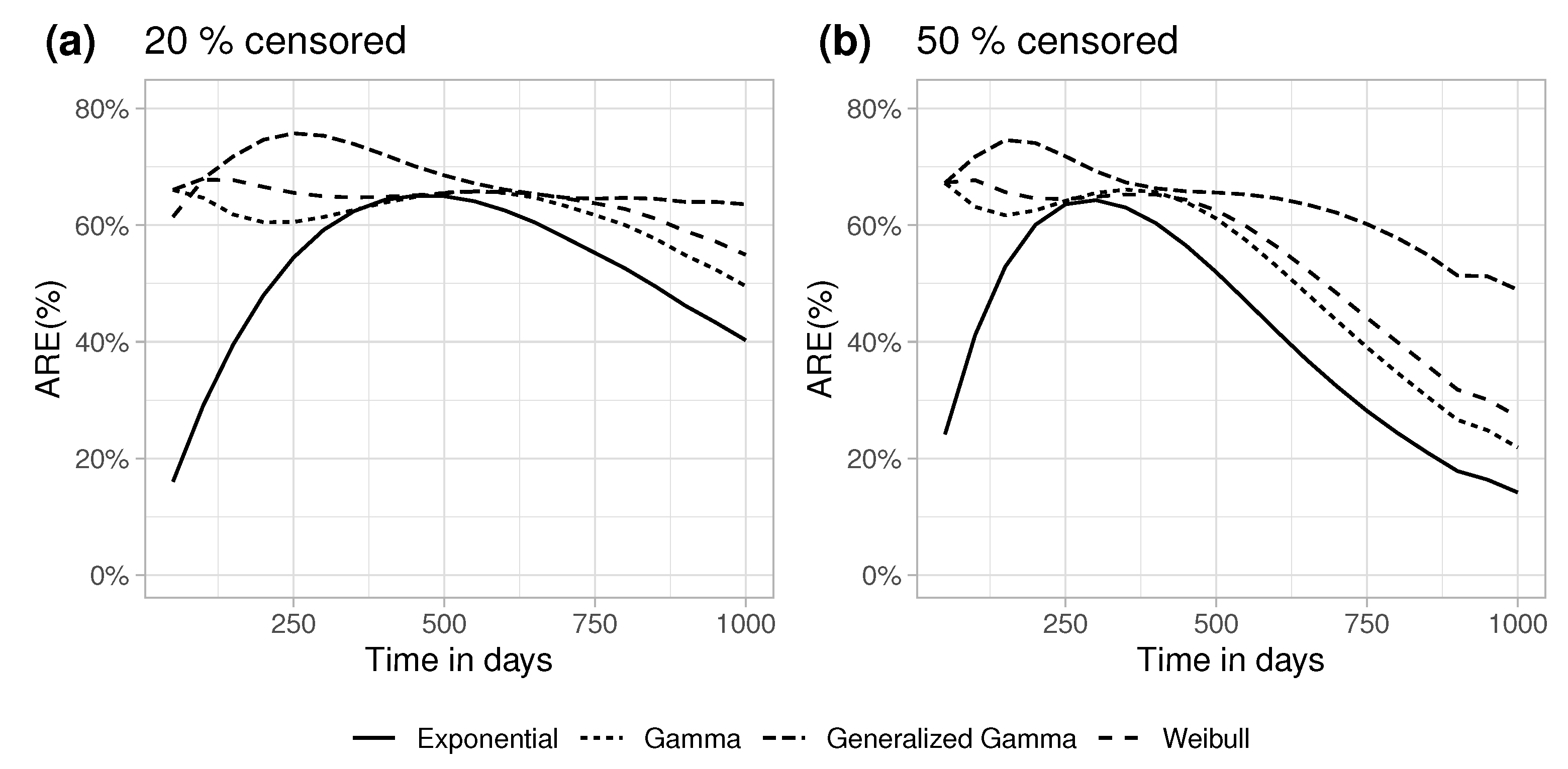
A set of simulations was run to illustrate the effect of adding additional parameters to the parametric models. As previously, we have simulated 1000 observation with exponential survival times (rate of 1 / 365 ) and exponential censoring times (rate of 1 / 365 leading to 50% and 1 / 1460 leading to 20% cenoring). In addition to the Exponential distribution, we have used the Weibull, Gamma and Generalized Gamma distributions for estimation of survival probabilities and associated variances. These later three distributions are extensions of the Exponential distribution with the addition of a power parameter (Weibull), convolution parameter (Gamma) or both (Generalized Gamma) [30], and if these additional parameters equal 1 then they simplify to the Exponential distribution. Thus, all three are consistent estimators of the survival probability. Figure A3 summarises the results of 1000 simulations. As expected the A R E for Kaplan–Meier estimator increases as additional parameters added to the parametric models. While A R E against the Exponential model followed what Equation (18) showed, the Kaplan–Meier estimator had better efficiency when compared against the Gamma, Weibull, and especially the three-parameter generalized Gamma distribution. This results are expected and the loss in efficacy generally becomes small as the number of parameters in the parametric model increases [31]. In addition one can see that increase in censoring reduced the A R E of the Kaplan–Meier estimator.
Figure A3. Asymptotic Relative Efficiency of the Kaplan–Meier estimator against parametric models with moderate (a) and high censoring precentage (b).
Stats 06 00072 g0a3
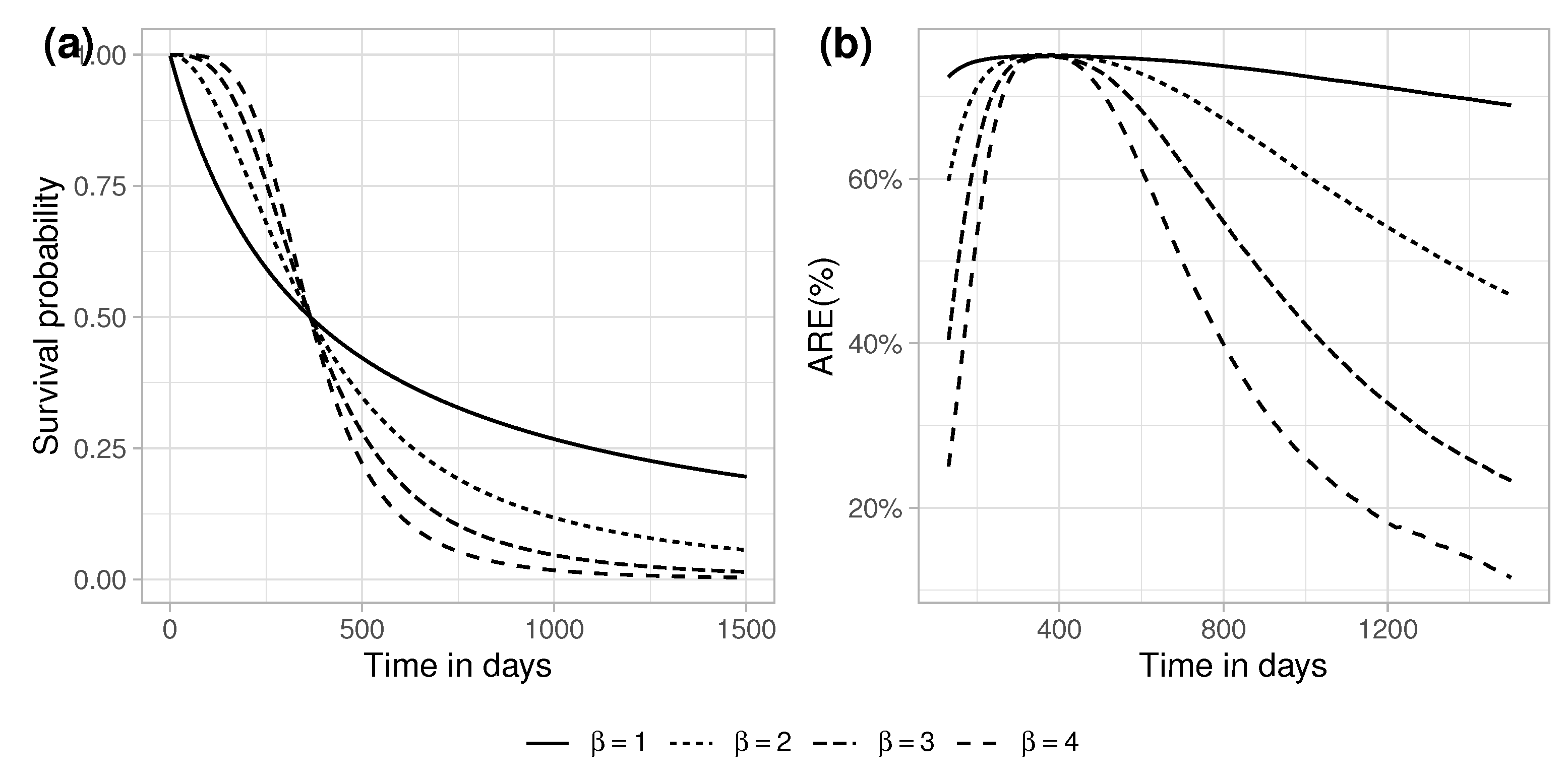
In addition to the three above mentioned distributions related to the Exponential distribution, we have tested the Log-logistic distribution. The log-logistic distribution is frequently used for events whose rate increases initially and decreases later, as, for example, mortality rate from cancer following diagnosis or treatment. The survival function is given by S ( t ) = 1 + ( t / α ) β 1 , β is the shape parameter and α is the scale. Both parameters are strictly positive and α is the median of the survival times and with increasing β the probability distribution of the survival a times are increasingly concentrated around α . In a simulation study we have set α = 365 and β = 1 , 2 , 3 , & 4 .
As it can be seen on Figure A4 a with increasing β the events are concentrated more and more around the median survival time. In addition with accelerated event rate the A R E of the Kaplan–Meier estimator rapidly approaches zero at the extremes of the survival time. At β = 1 the A R E of the Kaplan–Meier estimator stays in the vicinity of the maximum A R E of 75%.
Figure A4. Survival (a) and Asymptotic Relative Efficiency of the Kaplan–Meier estimator for Log-logistic survival times (b).
Stats 06 00072 g0a4

Appendix D. Correlation between Kaplan–Meier Survival Estimates at Different Time Points

Derivation of the correlation coefficient for Kaplan–Meier survival estimates at different time points largely follows Kaplan and Meier [1] (see Section 6.2 and Equations (2h) and (2g)), however with the notation updated according to Meier [22].
For survival times t 1 t 2 the correlation ( ρ ) between the Kaplan–Meier survival estimates is
ρ { S k m ( t 1 ) , S k m ( t 2 ) } = 1 S k m ( t 1 ) S k m ( t 1 ) S k m ( t 2 ) 1 S k m ( t 2 ) φ ( t 1 ) φ ( t 2 )
where φ ( t ) is the variance inflation factor of the binomial variance due to censoring. For any given t 1 the correlation between S k m ( t 1 ) and S k m ( t 2 ) decreasing with distance between t 1 and t 2 . This is easy to see, as with t 2 increasing S k m ( t 2 ) decreasing and S k m ( t 2 ) { 1 S k m ( t 2 ) } 1 is getting smaller. For survival times t 1 t 2 we have that φ ( t 2 ) φ ( t 2 ) so its easy to see that censoring further reduces correlation.

References

  1. Kaplan, E.L.; Meier, P. Nonparametric estimation from incomplete observations. J. Am. Stat. Assoc. 1958, 53, 457–481. [Google Scholar]
  2. Cox, D.R. Regression models and life-tables. J. R. Stat. Soc. Ser. B (Methodol.) 1972, 34, 187–202. [Google Scholar] [CrossRef]
  3. Hjort, N.L. On inference in parametric survival data models. Int. Stat. Rev./Rev. Int. Stat. 1992, 60, 355–387. [Google Scholar] [CrossRef]
  4. Miller, R.G., Jr. What price Kaplan–Meier? Biometrics 1983, 39, 1077–1081. [Google Scholar] [CrossRef]
  5. Klein, J.P.; Moeschberger, M.L. The robustness of several estimators of the survivorship function with randomly censored data. Commun. Stat.-Simul. Comput. 1989, 18, 1087–1112. [Google Scholar] [CrossRef]
  6. Aranda-Ordaz, F.J. Relative efficiency of the Kaplan–Meier estimator under contamination: Relative efficiency of the kaplan-meier. Commun. Stat.-Simul. Comput. 1987, 16, 987–997. [Google Scholar] [CrossRef]
  7. Meier, P.; Karrison, T.; Chappell, R.; Xie, H. The price of Kaplan–Meier. J. Am. Stat. Assoc. 2004, 99, 890–896. [Google Scholar] [CrossRef]
  8. Jullum, M.; Hjort, N.L. What price semiparametric Cox regression? Lifetime Data Anal. 2019, 25, 406–438. [Google Scholar]
  9. Cheng, P.E.; Lin, G.D. Maximum likelihood estimation of a survival function under the Koziol-Green proportional hazards model. Stat. Probab. Lett. 1987, 5, 75–80. [Google Scholar]
  10. Klein, J.P. Small sample moments of some estimators of the variance of the Kaplan–Meier and Nelson-Aalen estimators. Scand. J. Stat. 1991, 18, 333–340. [Google Scholar]
  11. Zheng, G.; Gastwirth, J.L. On the Fisher information in randomly censored data. Stat. Probab. Lett. 2001, 52, 421–426. [Google Scholar] [CrossRef]
  12. Zheng, G.; Balakrishnan, N. Fisher Information: Nonstandard Situations. In Wiley StatsRef: Statistics Reference Online; John Wiley & Sons, Inc.: Hoboken, NJ, USA, 2014. [Google Scholar]
  13. Nadarajah, S. Reliability for lifetime distributions. Math. Comput. Model. 2003, 37, 683–688. [Google Scholar] [CrossRef]
  14. Serfling, R. Asymptotic Relative Efficiency in Estimation. Int. Encycl. Stat. Sci. 2011, 23, 68–72. [Google Scholar]
  15. Nemes, S.; Gustavsson, A.; Taib, Z. Variance Inflation Due to Censoring in Survival Probability Estimates. Statistica 2020, 80, 395–412. [Google Scholar]
  16. Cramér, H. Mathematical Methods of Statistics; Princeton University Press: Princeton, NJ, USA, 1946. [Google Scholar]
  17. Cox, D.R. Principles of Statistical Inference; Cambridge University Press: Cambridge, UK, 2006. [Google Scholar]
  18. Peña, E.A.; Rohatgi, V.K. Small sample and efficiency results for the Nelson-Aalen estimator. J. Stat. Plan. Inference 1993, 37, 193–202. [Google Scholar] [CrossRef]
  19. Mardia, K.V.; Southworth, H.R.; Taylor, C.C. On bias in maximum likelihood estimators. J. Stat. Plan. Inference 1999, 76, 31–39. [Google Scholar] [CrossRef]
  20. Xuemao Zhang, S.P.; Wang, Y.G. Small sample bias correction or bias reduction? Commun. Stat.-Simul. Comput. 2021, 50, 1165–1177. [Google Scholar] [CrossRef]
  21. Geurts, J. Some Small–Sample Non–Proportional Hazards Resulis For The Kaplan–Meier Estimator. Stat. Neerl. 1985, 39, 1–13. [Google Scholar] [CrossRef]
  22. Meier, P. Estimation of a distribution function from incomplete observations. J. Appl. Probab. 1975, 12, 67–87. [Google Scholar] [CrossRef]
  23. Noether, G.E. On a theorem of Pitman. Ann. Math. Stat. 1955, 26, 64–68. [Google Scholar] [CrossRef]
  24. Van Eeden, C. The relation between Pitman’s asymptotic relative efficiency of two tests and the correlation coefficient between their test statistics. Ann. Math. Stat. 1963, 34, 1442–1451. [Google Scholar] [CrossRef]
  25. Jullum, M.; Hjort, N.L. Parametric or nonparametric: The FIC approach. Stat. Sin. 2017, 27, 951–981. [Google Scholar] [CrossRef]
  26. Nemes, S.; Gustavsson, A.; Jauhiainen, A. Focused Information Criterion for Restricted Mean Survival Times: Non-Parametric or Parametric Estimators. Entropy 2022, 24, 713. [Google Scholar] [CrossRef] [PubMed]
  27. Gebski, V.; Garès, V.; Gibbs, E.; Byth, K. Data maturity and follow-up in time-to-event analyses. Int. J. Epidemiol. 2018, 47, 850–859. [Google Scholar] [CrossRef] [PubMed]
  28. Boos, D.; Stefanski, L. Essential Statistical Inference: Theory and Methods; Springer: New York, NY, USA, 2013. [Google Scholar]
  29. Reid, N. Influence Functions for Censored Data. Ann. Stat. 1981, 9, 78–92. [Google Scholar] [CrossRef]
  30. Marshall, A.W.; Olkin, I. Life Distributions; Springer: Berlin/Heidelberg, Germany, 2007; Volume 13. [Google Scholar]
  31. Efron, B. Logistic regression, survival analysis, and the Kaplan–Meier curve. J. Am. Stat. Assoc. 1988, 83, 414–425. [Google Scholar] [CrossRef]
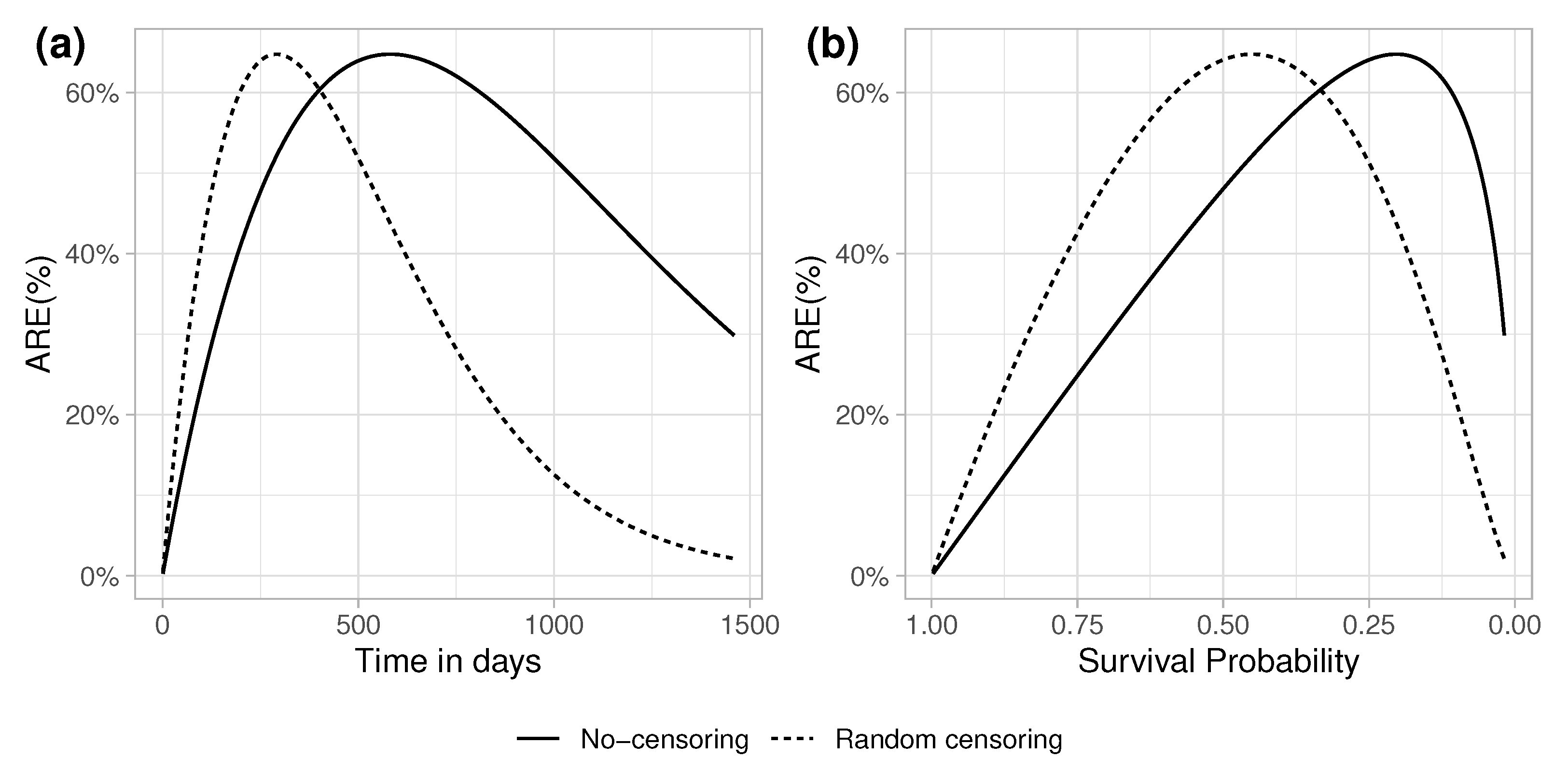
Figure 1. Numeric illustration of the Asymptotic Relative Efficiency (ARE) of the Kaplan–Meier estimator relative to the maximum likelihood estimator with a known exponential distribution with a rate of 1/365; ARE as a function of time (a) and as a function of survival probabilities (b).
Stats 06 00072 g001
Figure 2. (a) Numeric illustration of the Asymptotic Relative Efficiency (ARE) of the Kaplan–Meier estimator relative to the maximum likelihood estimator with known exponential distribution with rate of 1/365 at time of the Type I censoring; ARE as a function of time (a) and as a function of survival probabilities (b).
Stats 06 00072 g002
Table 1. Ratio of variances for Kaplan–Meier and parametric survival estimates for exponential survival times with a median survival time of 365 as a function of sample size and the procentual deviation for A R E in parenthesis.
Nt = 50t = 180t = 365
ARE12.7838.1558.20
2516.35 (27.92%)40.63 (19.4%)59.15 (7.45%)
5014.89 (16.49%)39.32 (9.15%)58.67 (3.70%)
7514.03 (9.77%)39.09 (7.35%)58.48 (2.21%)
10013.65 (6.79%)38.65 (3.91%)58.31 (0.88%)
12513.57 (6.17%)38.69 (4.22%)58.51 (2.44%)
15013.35 (4.45%)38.61 (3.59%)58.41 (1.66%)
20013.22 (3.43%)38.44 (2.26%)58.34 (1.11%)
25013.11 (2.57%)38.27 (0.93%)58.30 (0.37%)
100012.89 (0.85%)38.23 (0.62%)58.23 (0.25%)
Disclaimer/Publisher’s Note: The statements, opinions and data contained in all publications are solely those of the individual author(s) and contributor(s) and not of MDPI and/or the editor(s). MDPI and/or the editor(s) disclaim responsibility for any injury to people or property resulting from any ideas, methods, instructions or products referred to in the content.