1. Introduction
The consideration, collection and importance of data and their analysis is gaining more and more attention in many different fields—as it does in several sports disciplines. For example, in US sports such as baseball, basketball and American football, data regarding many aspects of a game, team or player have been recorded for many years. This trend can be observed in other areas of sports such as athletics, as well. Thus, statistical methods and analysis have become a topic of growing interest, and an interesting part in sports analysis are predictions and forecasts.
Among many other authors and articles on statistical methodology in sports, we refer to some of them. Based on results for order statistics and record values, Noubary [
1] proposed methods to forecast athletic records. Several authors applied extreme value theory. In Einmahl and Magnus [
2], the authors examined and compared world records in athletics based on extreme value theory, and they forecast the ultimate record in a specific discipline. By this, they initiated a series of subsequent works in this area. Noubary [
3] was concerned with athletic records and calculated the probabilities of future best performances based on tail estimation in extreme value theory. Einmahl and Smeets [
4] estimated ultimate world records for the 100 m running of women and men. Henriques-Rodrigues et al. [
5] focused on the semiparametric estimation of the extreme value index and of the right endpoint of the underlying distribution in case it was finite. The ultimate record in men’s long jump was examined in Fraga Alves et al. [
6]. Annual best times were used in Stephenson and Tawn [
7] to fit a model based on extreme value distributions to come up with extrapolated values which served as predicted records. Adam and Tawn [
8] considered annual records in athletics and swimming disciplines and fitted the parameters of the generalized extreme value distribution as underlying distribution.
A variety of other approaches for data from, e.g., baseball, football and athletics, can be found in the literature. As examples, we refer to Albert et al. [
9] and Wunderlich and Memmert [
10].
In contrast to forecasting procedures via extreme value theory in the sense of a long-term prediction by determining an extreme value distribution, the focus of our approach is on statistical prediction of the next record or records by means of previous record values in a particular sports discipline. We first repeat properties of upper and lower record values while focusing on lower records. We use the maximum product of spacings prediction procedure to derive a point predictor of the next record value based on previous ones, which are usually recorded. In the statistical model, we assume the lower/upper record values to be based on a sequence of independent and identically distributed random variables having a power function distribution/Pareto distribution due to our focus on explicit statistical prediction methods. Then, we derive some exact and approximate prediction intervals. We compare these intervals with regard to their expected lengths, and we analyze their percentages of coverage in a simulation study. We apply our results to real data from women’s 100 m and various other disciplines of athletics as well as to American football data by considering the evaluation of players by assigning so-called fantasy football points to players’ actions. Moreover, we discuss the distributional assumptions.
2. Prediction of Record Values
We first recall some basic properties of record values. For details, we refer to the monograph of Arnold et al. [
11].
Let
be a sequence of independent and identically distributed (iid) random variables with absolutely continuous cumulative distribution function (cdf)
F and probability density function (pdf)
f. Here,
denotes the set of positive integers. The random variables
are called upper record times. The random variables
,
, are then called upper record values. Analogously, the lower record times
are used to define the sequence of lower record values
,
. The joint densities for the first
upper and lower record values
and
are given by
where
and
where
, respectively.
It is well known that, in distribution, the upper record values
as well as the lower record values
can be simultaneously expressed by independent and identically standard exponentially distributed random variables
via
where
denotes equality in distribution (see Arnold et al. [
11]).
Aiming at deriving explicit statistical procedures, we choose power function distributions in case of lower records and Pareto distributions in case of upper records as underlying distributions; both families of distributions turn out to have a good fit to various data sets in sports. For parameters
and
, the cdf and pdf of the power function distribution
are given by
and, for parameters
and
, the cdf and pdf of the Pareto distribution
are given by
In the sequel, we assume the parameters and to be unknown and the (threshold) parameters and to be fixed.
There is a close relationship between power function and Pareto distributions, namely, if
holds then
follows, where
and
. Because of this relationship, we get consistent results for running (looking for minimum times), throwing and jumping events in athletics (looking for maximum lengths, widths and heights) without transforming times in velocities, as, e.g., in Einmahl and Magnus [
2].
2.1. Point Prediction
We consider point prediction of future record values based on previous records in a sequence of iid random variables. Among others, Kaminsky and Rhodin [
12] presented the maximum likelihood predictor (MLP) and Volovskiy and Kamps [
13] introduced the maximum observed likelihood prediction (MOLP). Based on a Pareto distribution, the MLP and MOLP for upper record values were shown in Volovskiy and Kamps [
14]. However, both methods share the disadvantage that neither the next upper nor the next lower record value can be predicted reasonably, since the methods lead to the last record as predictor of the next one. Raqab et al. [
15] derived the MLP and the so-called conditional median predictor. Moreover, there are some Bayesian results for estimation and prediction in the upper record Pareto setting in Ahmadi and Doostparast [
16], Madi and Raqab [
17] and Raqab et al. [
15]. For further references, we refer to Volovskiy and Kamps [
13] and Volovskiy and Kamps [
14].
We applied the maximum product of spacings prediction (MPSP) procedure for lower record values along the lines of Volovskiy and Kamps [
14] for upper record values. The idea underlying the MPSP method is to apply a transformation to the sequence
of observed records
,
as well as the yet-to-be-observed record values up to
, such that the transformed random variables are distributed as order statistics
from an iid sample of
uniform random variables. Then, by considering the spacings of the observed data after applying the transformation, the MPSP method chooses the prediction value
for the record value
that renders the observed data as uniform as possible according to some measure of uniformity. For a related estimation method in parametric inference utilizing the probability integral transform, we refer to Cheng and Amin [
18] and Ranneby [
19].
In what follows, we assume that the observed record values are from a sequence of iid random variables with continuous cdf
, which may depend on an unknown parameter
, where
denotes the set of parameters. Let
denote the function
,
. Then, Equation (
3) reveals that
where
is the sequence of upper record values in an iid sequence of standard exponential random variables. Reasoning as in Volovskiy and Kamps [
14], we conclude that
As mentioned above, the prediction of the
sth record is assumed to be based on observations of the record values
. Since the expected values of the order statistics
are equidistantly arranged in the interval
, Equation (
7) motivates the following inferential procedure for the future realization of
: using the notational convention that, for an interval
and
,
, for
, we define
and
and we call any function
a maximum product of spacings predictor of
if, for a suitable function
, we have that
and
maximize
, i.e., for any
,
and
where
and
denote the left and right endpoint of
, respectively. Note that the maximization of
with respect to
is necessary since
is considered to be unknown. However, given that in the present situation our focus is exclusively on predictive inference, the main object of interest is the point predictor given by the function
. By actually carrying out the above maximization, one obtains that the MPSP of
takes the form
where the function
is such that, for any
,
and
The proof of Equation (
8) proceeds along the same lines as the proof of (Volovskiy and Kamps [
14], Theorem 2.3). The maximum product of spacings prediction procedure is applied to the problem of sports records prediction in
Section 3.
In the particular situation of an underlying power function distribution as in Equation (
4), one easily sees that, for any sequence of observed lower record values
, the objective function
is independent of the shape parameter
, since the ratio in Equation (
7) is
Consequently, according to Formula (
8), the MPSP of
is given by
The MPSP is based on the ratios of evaluated for certain arguments. Hence, in the power function situation, the shape parameter drops out.
Analogously, the MPSP of the
sth upper record value in a Pareto distributed sequence of random variables is given by
It should be noted that the threshold parameters and are supposed to be known.
2.2. Interval Prediction
There are only a few articles in the literature dealing with prediction and prediction intervals for lower record values. In one of them, Wang et al. [
20] discussed estimation and prediction in a lower record setting with a baseline cdf
for
with parameters
from the proportional reversed hazard family, where
is a cdf itself depending only on the parameter
.
Prediction intervals for upper record values have been studied in several articles. For example, Awad and Raqab [
21] compared different intervals for records based on an exponential distribution. Asgharzadeh et al. [
22] and Raqab et al. [
15] introduced some intervals for upper record values from Pareto distributions. The intervals for lower record values proposed in this section are similar to those in the aforementioned articles and are applied to sports data in
Section 3.
2.2.1. Lower Record Values from Power Function Distributions
According to Equation (
2), the density of the first
r lower record values is
From the log-likelihood function
we obtain the maximum likelihood estimator
of
, which is required in the sequel.
In order to derive some prediction intervals for future lower record values, we examine the statistic
By using Equation (
3), one gets
Since the
are standard exponential random variables, the sums in the numerator and denominator follow a gamma distribution. Furthermore, the sums in the latter expression are independent, and, after scaling, we find
where
denotes an F-distribution with respective degrees of freedom. Now, we can compute a
-prediction interval for the
sth lower record value by using F-quantiles, namely
where
. Next, we consider
Hence, a
-prediction interval is given by
A generalized version of the statistic
is used in Wang et al. [
20] in a setting with unknown parameter
. For a known parameter
, prediction interval
will be applied instead of
.
In addition to those exact intervals, we study some approximate
-prediction intervals based on statistics similar to
and
, starting with
. It follows that
where
denotes a
-distribution with respective degrees of freedom. Plugging in
for
leads to the approximate
-prediction interval
containing
-quantiles. Furthermore, we consider the statistic
. From Equation (
3), one gets
and plugging in
, leads to
as an approximate
-prediction interval.
The prediction intervals are compared via the expected length and coverage percentage in a simulation study below.
2.2.2. Upper Record Values from Pareto Distributions
The corresponding prediction intervals for upper record values based on Pareto distributed random variables can be obtained analogously and are given by
was introduced in Asgharzadeh et al. [
22].
and
can be derived from the corresponding intervals in Awad and Raqab [
21] via an analogous formulation of the transformation in Equation (
6) for upper record values. Raqab et al. [
15] proposed
.
2.2.3. Expected Lengths of Prediction Intervals
For the expected lengths of the prediction intervals , , for future lower record values, the following expressions can be derived.
According to Equation (
3), the expectation of the upper bound of
is given by
In the last step, it was used that the moment-generating function of a standard exponential random variable
Z takes the form
for
. Hence,
The expected lengths of the other prediction intervals can be calculated similarly. They are given by
In the comparisons of prediction intervals, we restricted ourselves to the most relevant cases in practice, namely
and
. Moreover, as examples, we chose the parameters as
and
, which corresponded to the women’s 100 m and the men’s 400 m, respectively (see
Table 1 and
Table 2 and
Section 3).
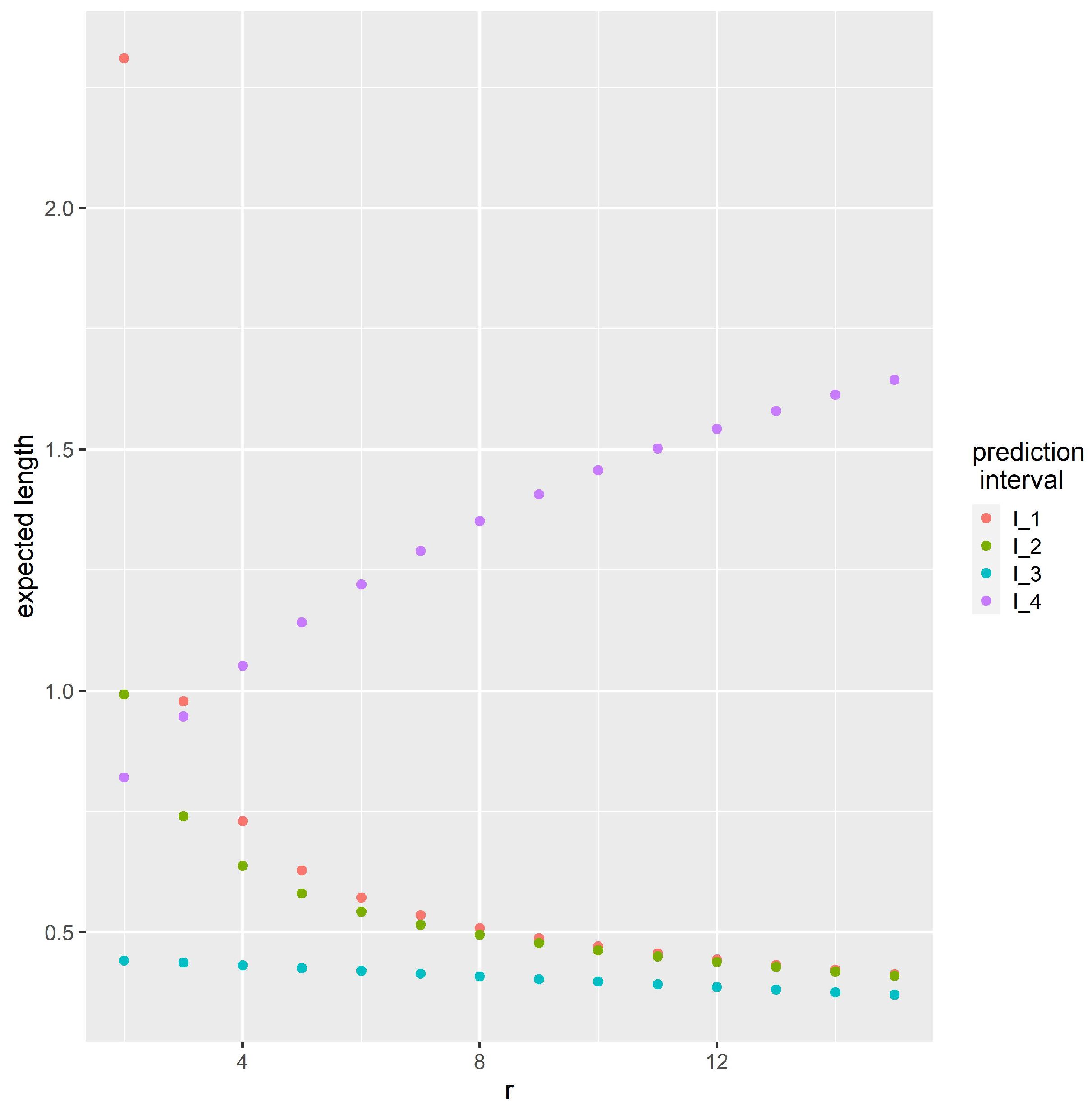
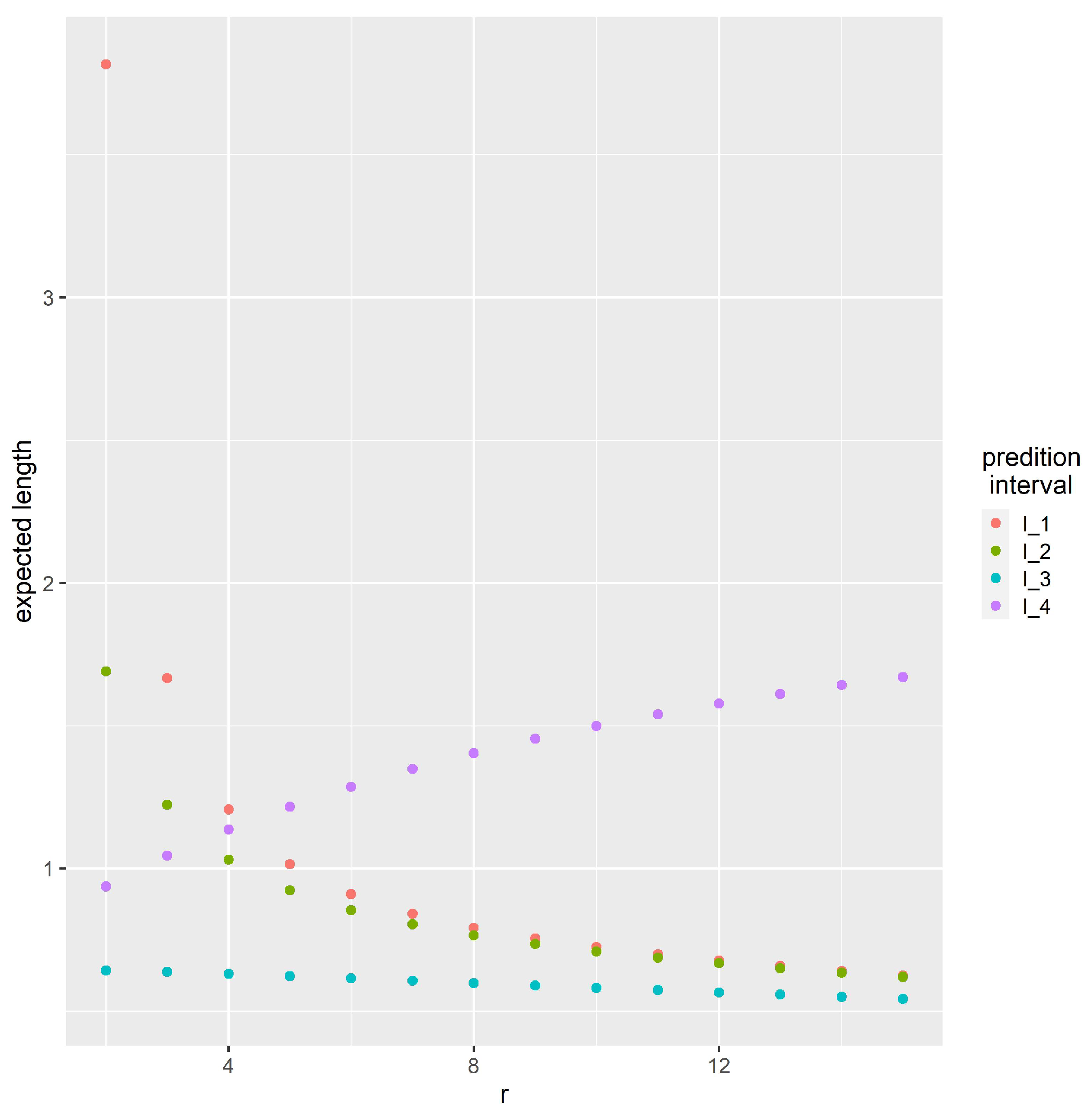
In
Table 1, the expected lengths of the prediction intervals
are shown for the two chosen parameter combinations and for different values of
r and
s. The prediction interval
which uses
as a known parameter outperforms
, where the first record value is used. Compared with the other intervals,
has large expected lengths, which are even increasing in the number of record values used in the prediction method. The asymptotic method
tends to have slightly shorter prediction intervals than the exact ones,
and
.
Figure 1 and
Figure 2 illustrate the expected lengths of all intervals for
and
, respectively.
We performed a simulation study concerning the percentages of coverage of the prediction intervals. We generated
n = 10,000 sequences of record values from a power function distribution and considered the first
r record values as known and the remaining records as unknown. Then, we computed the four prediction intervals based on these sequences and their empirical percentages of coverage. The results in
Table 2 show that the empirical coverage of the exact prediction intervals
and
was always close to
. As observed in
Table 1,
had small expected lengths, which corresponded to percentages of coverage (considerably) smaller than 90%, throughout. The asymptotic prediction interval
turned out to be too conservative. Summarizing, the exact prediction intervals
and
seemed to outperform the approximate approaches
and
.
3. Application to Athletics and American Football Data
Records play an important role in athletics. We applied statistical prediction methods for future lower and upper record values, namely, future world records, in athletic events, and we focused on the respective next record, i.e.,
was chosen. We assumed that lower records, as in running events, were based on a power function distribution, and that upper records, as in throwing and jumping events, were based on a Pareto distribution. These assumptions have to be justified in a given data situation. As an example, we considered the women’s 100 m; data of this discipline have been studied by extreme value methods before (Einmahl and Magnus [
2], Einmahl and Smeets [
4], Stephenson and Tawn [
7]). We used the data provided at
https://www.worldathletics.org/records/all-time-toplists, accessed on 19 December 2019. These data contain the personal bests of respective athletes, and we considered results until 2018. Since the times were taken with an accuracy of 0.01 s, we further adjusted those times in order to eliminate ties as in Einmahl and Magnus [
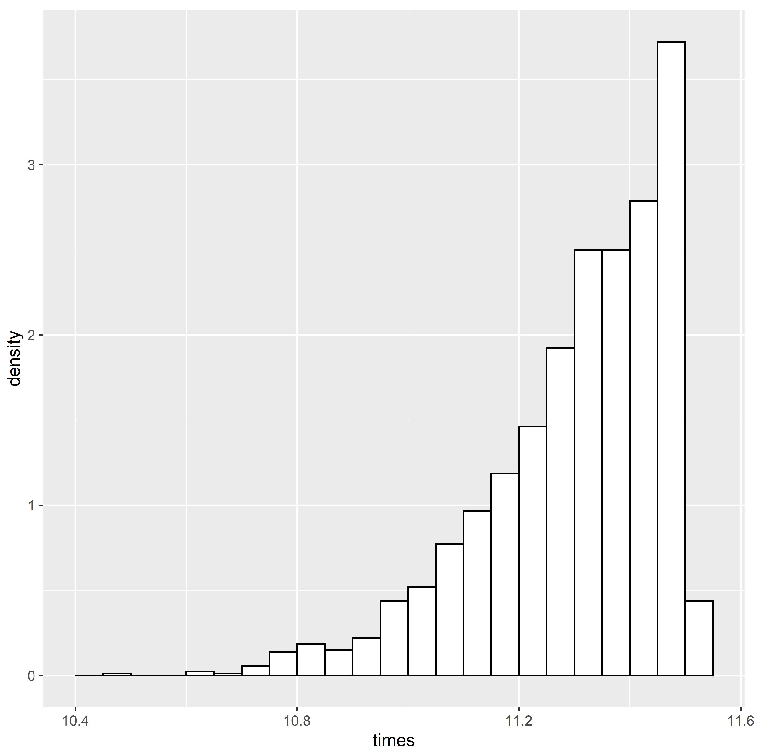
2]. A histogram of these slightly modified times is given in
Figure 3.
The common record model as introduced in
Section 2 is based on a sequence of iid random variables. While the assumption of independence seems to be reasonable, the assumption of identical distribution is questionable due to a possible trend in the data over time. In what follows, we stick to the iid situation. For the reason of comparability of sports results and in order to better approximately meet the assumption of identical distributions, we considered the times of top athletes only, whose running times were below a given threshold. In
Figure 4 and in our prediction results, this threshold was chosen to be
.
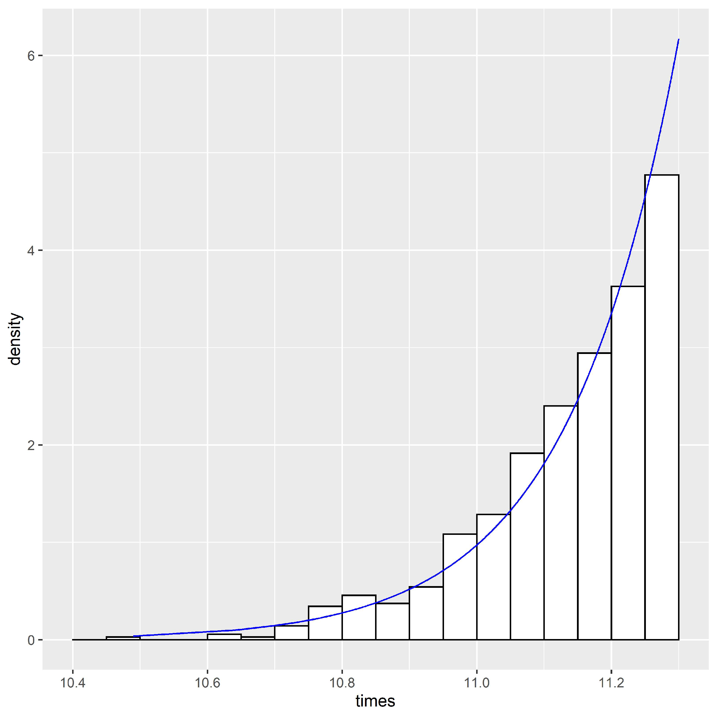
The curve in
Figure 4 illustrates the density function of a power function distribution with parameters
and
, where the latter value is a maximum likelihood estimate.
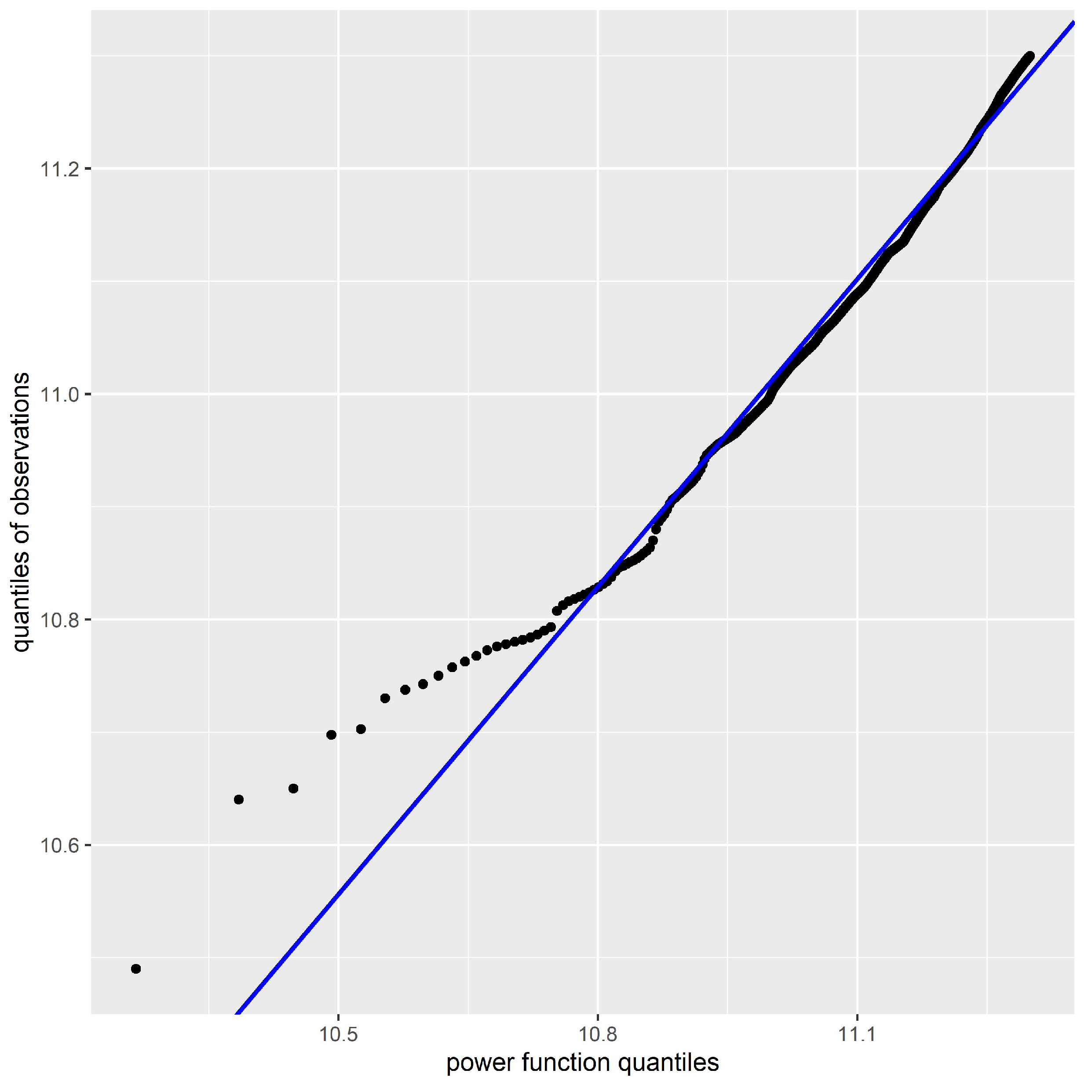
Figure 4 suggests that the power function assumption seems to be reasonable. However, the respective quantile–quantile (Q–Q) plot in
Figure 5 gives rise to question the assumptions.
Maybe the power function assumption should be modified as the smallest values indicate, or the assumptions of independence and identical distributions should be modified. Nevertheless, due to the histogram plot and for illustration of our theoretical results, we stuck to the power function assumption.
Then, we applied the point predictor MPSP for lower and upper records and the prediction intervals
/
,
/
and
/
, which were shown in
Section 2. The world record progression for the different events was recorded in
https://www.worldathletics.org/records/by-category/world-records, accessed on 25 November 2022. Unfortunately, not all of these lists were consistent. For example, some times in the running events were measured by hand and therefore had an accuracy of 0.1 instead of 0.01 for electronically measured times. In this listing, a record of 11.20 was regarded as faster than the old record 11.1 for the women’s 100 m. To avoid such data problems, we excluded times measured by hand. To illustrate the prediction results,
Table 3 shows world records in the women’s 100 m along with respective MPSP and prediction intervals
,
and
based on the previous record values. The point predictor (MPSP) and the prediction interval shown in row
i of
Table 3 are based on the previous records listed in rows
,
.
It can be observed that most world records were close to the MPSP and were within the prediction intervals. An exception was the record ran by Florence Griffith-Joyner in 1988. It was considerably smaller than the MPSP and the lower bound of the statistical prediction intervals. Moreover, such an exceptional record had a strong effect on the statistical prediction of subsequent record values.
By using the same procedure in other running events and an analogous approach for upper records in throwing and jumping events with underlying Pareto distributions, where the distributional assumption was approximately met, we derived the results shown in
Table 4.
Obviously, the number of world records was small in the women’s 800 m, 1500 m, marathon and javelin throw. Therefore, the predictions in
Table 4 may differ from the actual next record. Moreover, the respective prediction intervals were quite large. For example, the lower bound for the next marathon record was nonsatisfying.
However, in the men’s marathon, the lower bound was smaller than two hours as well. The number of records was , so the prediction interval was expected to be quite reasonable having a lower bound below the two-hour mark. In October 2019, the world record holder Eliud Kipchoge broke this mark under special conditions regarding, for example, the course, wherefore it was not considered an actual world record.
In general, prediction intervals tend to be large, if the number of observed records is fairly small. Thus, in such a real data situation, the prediction interval may not be of practical use (see
Table 4).
In addition to the analysis of athletic events, we applied point and interval prediction to data from American football. A possible data set could result from the NFL Combine with its athletics disciplines.
However, we focused on data resulting from actual football games in the NFL. To combine most relevant metrics in the analysis of a player’s performance on the field, we considered so-called fantasy football points (see, e.g.,
https://fantasy.nfl.com/research/scoringleaders, accessed on 2 March 2021). These fantasy points are calculated according to the points per reception (PPR) scoring scheme (see
Table 5 and the glossary at
https://www.pro-football-reference.com, accessed on 14 January 2020), for each game separately. Many providers of football data additionally offer fantasy points of players that are added up to a full season performance. Here, we focus on single game performances.
Related to these data of fantasy football points, we may define world records in American football. When measured by means of the PPR scheme, the respective world record performance (as of December 2019) by quarterback Michael Vick was composed of 333 passing yards, 4 passing touchdowns, 80 rushing yards and 2 rushing touchdowns in a single game, which yielded
We distinguished between the skill positions quarterback, wide receiver, running back and tight end. Other players such as linemen, defense players and special teams were not included in the analysis. The points of kickers and whole defense teams were measured in the standard scoring scheme as well, but they followed a discrete distribution and were therefore not considered here.
We determined the sequences of records for quarterbacks, wide receivers, running backs and tight ends as the basis for point and interval prediction. The underlying game data are provided at
https://www.pro-football-reference.com (accessed on 14 January 2020, publicly available until 2020) and cover each game of the regular seasons from 2000 to 2019. The fantasy football points were rounded to one digit for quarterbacks as well. The Pareto assumption could be justified by comparing the histogram and the estimated density function as above. Only for the tight end’s points did a Pareto distribution not seem to be reasonable. Since there were just two records in the wide receiver’s data, we did not compute predictions for this position either. The progressions of the world records and the corresponding predictions can be found in
Table 6 and
Table 7.
Using box score statistics such as fantasy points to measure a player’s performance has been discussed intensively, since it does not weight the yardage made by its effectiveness in a drive. Four yards at third and three are regarded as valuable as four yards at third and five, although the outcome of the play is different.
4. Discussion
We developed and applied point and interval prediction based on a sequence of lower or upper record values to various data sets from athletics and American football to come up with predictions of future record values. In the examples, these predicted values were successively compared with actual subsequent record values. Several prediction methods were discussed and results for lower record values were established, which were used, e.g., for analyzing data from running disciplines in athletics. The procedure as well as the results can also be applied to other sports disciplines. In the model of common record values, we assumed that the considered record values were smallest or largest observations of a sequence of independent and identically distributed random variables. In particular, this assumption of underlying identical distributions presumed that the athletes were able to perform on the same level. In order to approximately meet the assumption of identical distribution, we only considered results better than some threshold interpreted in such a way that we considered just top athletes and top performances. Here, we applied power function distributions with respect to lower record values and Pareto distributions with respect to upper record values, which often are seen to have a reasonable fit to the data. Of course, there are disciplines mentioned in this article, where the distributional assumptions are not really justified, such as in women’s 800 m and in tight end’s fantasy points. Moreover, certain dependencies within sports data cannot be avoided. For example, some sportspersons in athletics broke a record more than once and therefore, their names occur several times in the list of records. These results cannot be regarded as independent. However, if there are many people involved in a list of records, independence may be assumed at least approximately. Furthermore, in sports such as American football, there are dependencies among a team or between competitors. Despite some possible criticism on the model of common record values in sports applications, the prediction methods performed quite well. Most world records and point predictions lay within the respective prediction intervals. Prominent exceptions are, e.g., the records of Florence Griffith-Joyner in the women’s 100 m and Bob Beamon’s world record in the men’s long jump. Such exceptional performances were much better than expected and had a strong influence on statistical predictions.
