1. Introduction
The heterogeneity of economic development is an immanent property of the spatial organisation. The matters of mitigating social and economic inequalities are becoming relevant for Russia—a country of natural resource endowment, a vast territory with unequal population density and concentration of extractive industries.
In conditions of uneven economic development, income inequality is one of the most urgent issues not only in Russia but also in the world. Many studies explore intra- and interregional disparities and differences in data between centre and periphery come from China [
1,
2,
3,
4,
5], the United States [
6,
7,
8], Canada [
9,
10], India [
11], Brazil [
12], and European countries [
13,
14,
15].
Hierarchical interrelations in large countries, including Russia, both vertical (municipalities, regions and country) and horizontal (inter-municipal and inter-regional), actualises the study of inequality with the use of multilevel analysis, which takes into account the nested nature of data.
Multilevel modelling is actively applied to exploring income inequality and allows for developing differentiated management decisions in relation to each level of the administrative division of the country. The heterogeneity of the economic space and the different development paths of the south/north/east/west, urban/core and rural/peripheral areas within individual countries determine the prerequisites and factors of increasing/decreasing income inequality. Therefore, the factors must be considered in the territorial context [
9]. Recent studies highlight the following factors that influence the variance of the population income: level of social and economic development, sectoral structure of the economy, human capital and unemployment [
9,
12,
16,
17,
18]. Countries have different structures of population income and various shares of wage and social transfers in population income, which defines the need to study conditions and factors having an impact on wage variance [
19,
20,
21,
22,
23,
24]. The contribution of certain factors to interregional and intraregional inequalities depends on the local specifics of municipalities and the role of the regions in the national economy.
Our research enriches the existing body of the literature in terms of social inequality factors across Russian regions and municipalities, focusing on spatial effects and their relationships within the framework of multilevel models. It could be used as an initial background to study the causal relationships between social policy, transfers and population income.
Our research addresses the following questions: What factors matter in one group of regions but do not matter in the others? How do regional and municipal contexts simultaneously affect population income? The listed reasons determine the relevance of this research area, and our aim here is threefold, to determine:
- (1)
How do regions and municipalities contribute to the variances of population income and wages?
- (2)
What factors affect the variances of population income and wages?
- (3)
What is the relationship between population income, wages and transfers?
The remainder of the paper is organised as follows.
Section 2 provides a theoretical framework to study inequality in population income at a small scale and justifies using a multilevel approach.
Section 3 includes research design, where we present model specifications and justify each factor embedded into the model.
Section 4 introduces a brief description of the population income variance, results of population income and wages modelling, and highlights the main empirical findings, focusing on intra-regional and inter-regional variances.
Section 5 presents the discussion.
Section 6 concludes the paper.
3. Research Design
3.1. Multilevel Model with Cross-Classified Random Effects
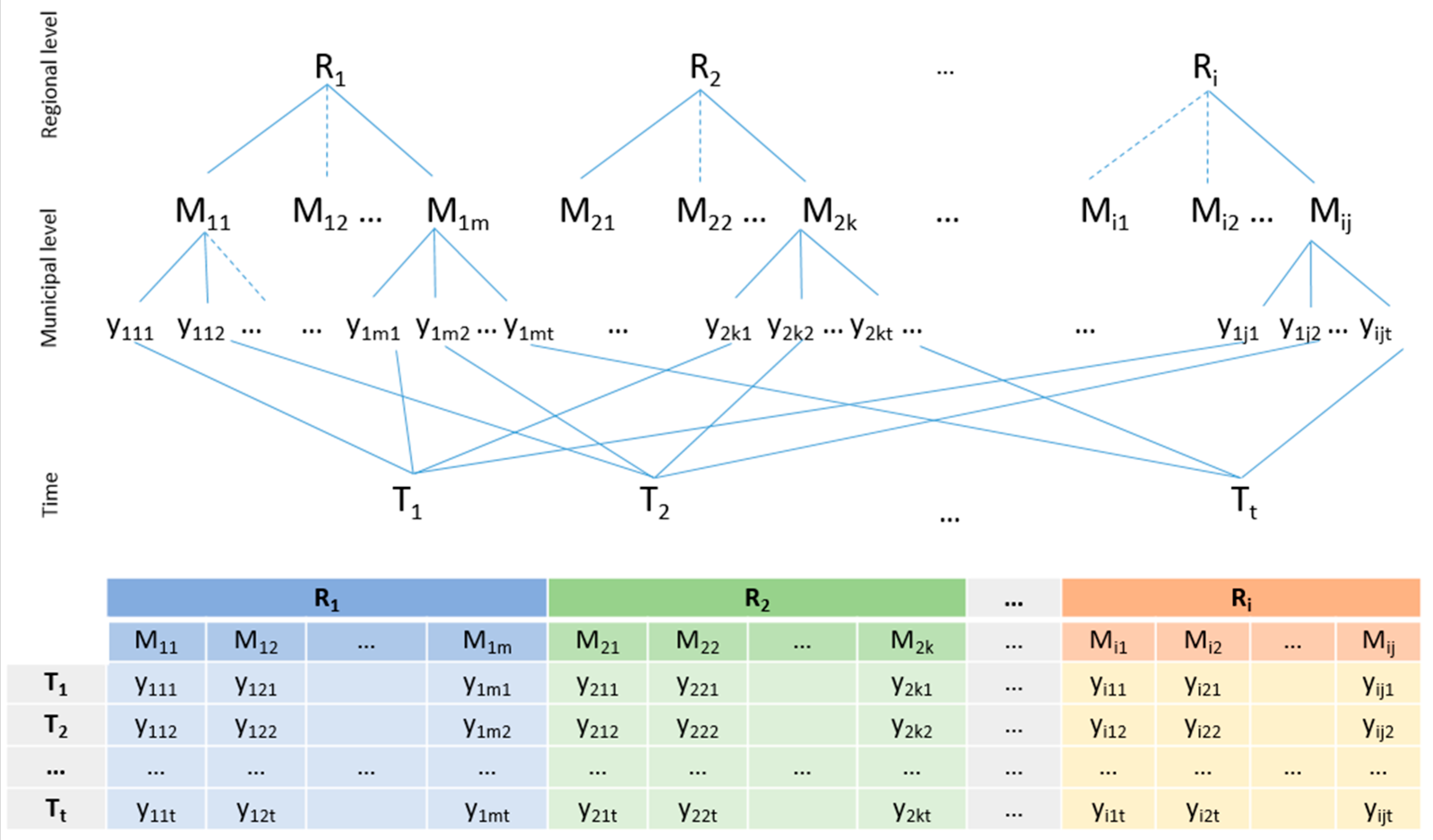
Our study analyses cross-classified effects formed in conditions when each value in the data set simultaneously refers to a certain municipality and a particular year of the study (
Figure 1). At the same time, the nesting of municipalities into regions (subjects of the Russian Federation) is taken into account in the data set.
A Hierarchical Linear Model with Cross-Classified Random Effects (HLMHCM) can be used to analyse the data grouped in this way. It has three submodels, within which the dependencies of level 1, level 2 and cross-classified random effects are considered.
The rationale for using hierarchical models is determined by the presence of group and intergroup variance and heterogeneity of data in the context of certain levels of territorial division (municipality, region). These differences can be revealed in various ways. We carried out Levene’s Test to check whether the variances between two or more groups are equal. Levene’s test was previously used for non-normally distributed data. Given the features of the analysed data, we additionally used the Figner-Killeen non-parametric test for abnormal data. The null hypothesis for each test: the variance among the groups is the same.
The multilevel approach involves the sequential construction of several models. In the first stage, we built a null model without predictors (model 1):
Level 1 (Municipal level):
Level 2 (Regional level):
Cross-Classified Effects:
where
Ymijt—dependent variable, characterising observation m related to
i-municipality (1…2016) nested in
j-region (1…75) in
t year (2015…2019).
—constanta;
rmijt—random effects for each observation m, where rmijt ~ N(0, σ2);
ε0jt—random effects for each municipality i, where ε0jt ~ N(0, τ2);
φ000j—random effects for each region j, where φ00jt ~ N(0, ej2);
π000t—random effects for each year t, where π00jt ~ N(0, et2).
The values of obtained effects as a result of constructing the null model were used to estimate the contribution of each level to the overall variance of the dependent variable by estimating the share of
σ2,
τ2,
ej2,
et2 in the total sum of effects. The intra-unit correlation coefficient (
IUCC) is represented as follows [
46]:
IUCC allows for identifying to what extent the variance of the examined indicator is determined by the chosen levels. The inclusion of predictors in subsequent models reduces the value of random effects as a result of their explanation of observed variance. Thus, within the framework of the null model, we consider the contribution of each level without specifying the factors associated with this contribution at each level.
Given the assumption that included factors enable us to explain the variance, we constructed model 2 on the next step (Equations (4)–(6)):
Level 1 (Municipal level):
Level 2 (Regional level):
Cross-Classified Effects:
where
Xmijt—independent variable attributed to municipality
i (1…2017) nested in region
j (1...75) in
t year (2015…2019), %;
Zjt—independent variable related to j-region (1...75) in t year (2015…2019), %.
The uneven development of a municipality is determined both by its own indicators and the region’s factors to which it belongs. In order to account for these relationships, the inter-level interaction was introduced into model 4, which allows for assessing coefficients related to municipal factors (Level 1) as a function of regions’ ones (Level 2). Given the included estimates of the inter-level interaction of indicators, model 4 has the following form (Equations (7)–(10)):
Level 1 (Municipal level):
Level 2 (Regional level):
Cross-Classified Effects:
The models were compared according to the logarithm of likelihood, Akaike criteria (AIC), Schwartz (BIC) and deviation (DIC). All the above models are estimated using Restricted Maximum Likelihood (REML) and Maximum Likelihood (ML). REML estimation is preferable since it produces unbiased estimates for the random parameters, but it is inappropriate to perform likelihood-ratio tests for fixed effects when the model is fit by REML. Thus, for model exploration and hypothesis testing, ML was used, with a final REML estimation as recommended [
39]. DIC criterion is preferable to use for the comparison of multilevel models. DIC criterion takes into account model deviations, and unlike AIC, the DIC is based on a posteriori average when models with a smaller DIC are preferable [
47].
The analysis was carried out in the R environment using Car, lmer, EMAtools and lmerTest libraries.
3.2. Data Source
The analysis was carried out on the data of 2017 municipalities in the context of 75 regions of the Russian Federation in 2015–2019. The main data source is the database of municipalities formed by the Federal State Statistics Service of the Russian Federation (
https://www.gks.ru/dbscripts/munst/ (accessed on 1 June 2022)).
The regional-level data were obtained from sources of the Federal State Statistics Service (
https://rosstat.gov.ru/ (accessed on 1 June 2022)) and the Unified Interdepartmental Information and Statistical System (
https://www.fedstat.ru/ (accessed on 1 June 2022)). This data set covers 86% of the municipalities in Russia. The characteristics of the indicators are presented in
Table 1 and
Appendix A.
3.3. Factors Determining the Variance of Population Income
This study is aimed at exploring contextual factors that determine the difference in population income across the regions of the country.
We take the volume of social transfers and taxable income of the population across municipalities (municipal districts, urban districts) as a dependent variable characterising population income within the municipal district (city district) boundaries (variable Income per capita). This variable comprises:
- -
Personal income, including wages and incomes of individual entrepreneurs;
- -
Pension, social transfers and benefits, including unemployment allowance, social benefits and assistance measures, benefits and compensations to military personnel, maternity benefits, child care and other "child" benefits;
- -
Insurance indemnities; lottery winnings; interest on deposits, and compensation for deposits, scholarships, and money transfers.
The average value of social transfers and taxable income per capita was obtained by dividing the amount of the volume of social transfers and taxable income by the total population of municipalities. In order to obtain comparable types of indicators, their nominal values were adjusted for the price indices for goods and services. Since the Federal Statistics Service does not estimate these price indices at the municipal scale, we used regional price indices for goods and services.
Recent studies underlined several groups of factors that determine differences in population income. Our research embraces data aggregated at both the municipal and regional levels, which was publicly available. All variables are in comparable form due to their adjustment for the price indices for goods and services.
3.3.1. Economy of Territory and Its Structure
The sources of population income are different. The more economically developed the territory is, the more opportunities the population has to earn income. Traditionally, GRP per capita is a basic indicator of regional economic development [
5,
26]. Since this indicator is not collected at the municipal level, we used an indicator of the volume of goods, works, and services produced and shipped divided by the total resident population as an independent variable (variable Production per capita). The examined indicator does not include data on small business production because it is not collected at the municipal scale. In general, the share of small business production in Russia is quite small, and its absence does not distort obtained estimates.
Industry profitability varies significantly. The structure of the economy is considered through income disparities across industries [
9,
12,
16,
17,
18,
22]. Our study explores the share of employees in the following industries: agriculture and fisheries (variable EmpAgricultura), mining (variable EmpMining), manufacturing (variable EmpManufacturing), construction (variable EmpConstruction), catering and hotels (variable EmpCateringHotels). We have also included the number of entrepreneurs per capita to take into account the development of small businesses in the region’s economy (variable Entrepreneurship).
The study uses the population of the municipalities (variable Population size) as a variable characterising the size of the economy to control for agglomeration effects [
48] and allows us to gain a better understanding of the income inequality reasons [
17,
49,
50,
51].
3.3.2. Human Capital
Education is one of the most frequently used factors in exploring income inequality [
9,
17,
18,
48,
52]. Scientists separately consider the proportion of the population with higher secondary and primary education. Our study also separately explores the share of the employed population with higher education (variable High school), secondary education (variable College education), primary education and incomplete school (variable Elementary school). Education is considered to be an engine of innovation activity. The development and implementation of new technologies increase labour productivity and contribute to economic growth. Our study involves the volume of patents granted for inventions and utility models per 10,000 population as an indirect factor of human capital development (variable Patent).
In Russia, men and women have equal rights to work. However, due to various cultural and social reasons, women often prefer not to work and manage the household. At the same time, studies show that women’s economic activity has a positive effect on average income [
10]. Therefore, the analysis considers the level of women’s participation in the labour force (variable Female).
3.3.3. Income Inequality
Regional income disparities considered in the paper are closely associated with social imbalances. People with significant differences in income may live within the same territory, but average income may not reflect it.
Scientists underline the complex and contradictory relationship between income inequalities and GDP per capita [
16,
48,
52]. The state aims to alleviate income inequalities with transfers, but results are mixed because they influence the people’s need to work. Therefore, we consider two indicators: the Gini coefficient of population income (variable Gini) and the share of social transfers in the monetary population income (variable Transfers).
3.3.4. Spatial Correlations
Many studies emphasise the importance of including spatial correlation [
10,
52], which arises from the openness of the market economy with free-moving flows of capital and labour. The equilibrium in neighbouring markets is achieved faster because of filling vacancies with workers from areas in the vicinity. We included in the model the average volume of social benefits and taxable income of the population of municipalities in the neighbourhood (variable WIncome per capita).
A model that includes all the above-mentioned factors is presented as follows (Equations (11)–(15)):
Level 1 (Municipal level):
Level 2 (Regional level):
Cross-Classified Effects:
where
—constanta;
rmijt—random effects for each observation m, where rmijt ~ N(0, σ2);
ε0jt—random effects for each municipality i, where ε0jt ~ N(0, τ2);
φ000j—random effects for each region j, where φ00jt ~ N(0, ej2);
π000t—random effects for each year t, where π00jt ~ N(0, et2).
3.4. Factors Influencing the Wage Variance
The wage is a base of population income that depends on invested individual efforts; therefore, its exploration is an important component of population income analysis. We use the real average monthly wage of employees in organisations as a dependent variable (variable Average wages). This indicator is being collected at the municipal scale and embraces information on the average monthly wage in large, medium-sized and non-profit enterprises, including state-owned ones. At the same time, this indicator does not include data on the average monthly wages of small enterprises and entrepreneurial income. The value of the indicator is brought to the level of 2015 using the price indices for goods and services as in other studies [
24,
53].
The set of factors that influence the wage is, to a large extent, the same as that considered while analysing the volume of social transfers and taxable income of the population. However, numerous studies showed that some factors are more influential for wages [
19,
20,
21,
23,
24].
3.4.1. Labour Productivity and Unemployment
Labour productivity is considered to be tightly associated with wages [
20,
53,
54]. This close relationship is a long-running issue in economics, addressed both in theoretical and empirical studies [
53]. We calculated the variable Productivity by dividing the volume of goods, works, and services produced and shipped by the number of enterprises’ employees.
Unlike the model of income per capita that uses the volume of goods, works, and services produced and shipped divided by the total population as an independent variable, here we emphasise the volume of production provided by employees of enterprises because it better explains the relationship with salary. In a number of regions, the value of production per capita and the volume of production per employee does not coincide due to the differences between the number of enterprises’ employees and the local population. These differences are clearly visible in relation to the average number of enterprises’ employees and the resident population (variable Working population per capita) in the northern regions of Russia, where the resident population is small, and workers from other regions are being attracted to mining. In certain municipalities, the number of enterprises’ employees is 2.5 times more than the number of the resident population.
According to the laws of supply and demand, high unemployment negatively affects the wage because the population is ready to work at lower wages. Thus, we included unemployment (variable Unemployment) in the model similar to the other studies [
20,
21,
24,
53,
54,
55].
3.4.2. Spatial Autocorrelation of the Unemployment Rate and Wages
Alongside the unemployment rate within the region, we included unemployment in neighbouring regions as a factor in the analysis. Employers are less likely to lower wages in response to an increase in the local unemployment rate if they fear that their workers quit current jobs for similar ones in a neighbouring region [
55]. Thus, we incorporated into the analysis the average value of the unemployment rate in neighbouring municipalities (variable WUnemployment), which was assessed by multiplying the value of unemployment by a row-standardised, first-order adjacency matrix.
Exploring the spatial correlation of the unemployment rate, scientists underline the need to consider the share of the rural population because labour supply elasticity, measured by the share of the agricultural population in each area, explains wage differences [
56]. The population from rural areas often migrates to urban areas because it is easier to find work there. The unemployment rate is assumed to be lower in the city [
57]. Another reason to include the urban/rural share of the population in the analysis is that urban areas have higher wages (variable Urban/Rural) [
24,
58].
At the same time, scientists recommend taking into account average wages in neighbouring territories and controlling spatial effects [
23,
24,
54]. The openness of markets suggests the free movement of labour and, as a consequence, the wage balance within neighbouring territories. Our analysis considers the average spatial wage (variable WWage), obtained by multiplying the value of the average wage in municipalities by a row-standardised, first-order neighbourhood matrix.
3.4.3. Open Economy
The influence of neighbouring territories is not limited by the movement of labour. Regional economies are strongly linked, so the analysis of wages involves characteristics of the economy’s openness [
13] and market potential [
59].
Firstly, firms in remote areas are assumed to have greater transport costs on both exports and intermediate inputs, reducing the amount of value-added left to remunerate domestic factors of production, so they can only afford to pay relatively low wages in comparison with regions with high market access [
13].
Secondly, the economy’s openness provides wider opportunities for product sales to foreign markets and, consequently, an increase in profits. In particular, export activity in the region might encourage the creation of new jobs, a decline in the unemployment rate, and an increase in real wages [
57].
Recent studies show that the difference in regional economies’ openness is manifested in the variance in real wages. For instance, rising intermediate goods export openness in the last decade was a 23% increase in the average economy’s variance of real wages [
60].
We used two indicators to reflect economies’ openness in our study. The first indicator is the volume of exports which represents both possibilities of selling products to foreign markets and the economic potential of the territory (variable Export). The second one is a spatially weighted value of regional GRP as a characteristic of the local markets’ potential (variable WGRP). Spatially weighted distance allows considering the proximity of the sales market; therefore, when calculating this indicator, we take data from all regions, adjusted for the inverse distance to them [
13,
59].
3.4.4. The Structure of the Employed Population
The average wage in the region is largely connected with the industries in which employees are involved [
19,
20,
23,
24,
55,
56,
61]. Our study comprises the shares of employees in the agriculture and fishing (variable EmpAgricultura), mining industry (variable EmpMining), manufacturing industry (variable EmpManufacturing), catering and hotels (variable EmpCateringHotels).
We include several control variables in the study at the regional level to estimate the share of employees in small businesses: average number of employees of small and medium-sized enterprises to the total population (variable EmpSmallBusiness); the number of individual entrepreneurs per capita according to state registration data (variable Entrepreneurship). Small businesses are supposed to provide different employment opportunities and a variety of wage levels accordingly. Innovatively active small enterprises could have a higher level of wages. At the same time, recent studies indicate that the share of small firms may negatively affect the level of wages [
55].
Simultaneously with the industrial structure of the employed population, the current study examines the educational structure of the population. Recent studies showed the benefits of higher education ("education pays") in terms of salary [
23]; therefore, the wage model involves the share of employees with higher education [
13,
20,
23,
24,
53,
62]. Scientists also investigate such variables as college graduates per capita [
56], workers without education [
20], and the share of low-skilled workers in the total number of employees [
53]. Our study separately examines the proportions of the workers with higher education (variable High school) and post-secondary education (variable College education). Additionally, the model includes a variable Patent per capita to take into account the ability of employees to innovate, which may also influence the wage [
13].
Experience is often associated with the age of employees. Young workers have less work experience, and they often combine work and study. They usually earn less, so in a region with a large share of the younger population, the average wage may be lower [
24]. At the same time, they have better scores for mental speed and memory [
23]. Older employees with a lot of work experience have less physical strength and pay more attention to their health [
23]. Older employees do not tend to work too much; thus, lower average wages can also be expected in regions with a large proportion of older workers [
24]. Given these relationships, academics explore the causal links between wages and the shares of young [
19,
23,
24] and elderly [
20,
23,
24] people. Our research incorporates two variables, reflecting the role of labour force employees under 20 years of age (variable Younger) and over 50 (variable Older).
Labour force participation among women has a significant impact on the wage [
14,
20,
23,
55,
61]. Studies reveal a wage gap between men and women. As a result, an increase in the share of women in the labour force leads to a decrease in the average regional wage [
61]. An increase in the proportion of women affects labour supply elasticity [
23,
55].
3.4.5. Income Inequality
The average wage in the region is an aggregated indicator that does not reveal the degree of wage inequality at the individual level. Therefore, we added the Gini coefficient to the model (variable Gini). In most countries, the state tries to alleviate inequality in the living standard of the population through social transfers. Ideally, such compensation should not affect the labour-market arrangements. For example, Candelaria et al. [
56] reveal no correlation between real wages and government transfers; thus, the Chinese government does not compensate or exacerbate wage differences. In turn, studies on the data from the Russian Federation show a significant negative impact of regional subsidies on real wages in cities outside the Far North and the weakening effects of extractive industries on real wages [
37]. We included the share of social transfers in the total monetary population income in the analysis (variable Transfers).
3.4.6. Working Conditions and the Trade Union Activity
We consider two factors that are rarely considered in the scientific literature, but they need testing. First, it should be taken into account that not only the educational level but also hazardous working conditions increase salary.
Hazardous working conditions can be associated both with work in very cold areas, at height, and in an area harmful to health. In particular, there are high health risks in the areas of high radiation or in chemical industries. Conducted research showed that working conditions had no significant effect on individual wages in the labour market, whereas hazardous working conditions significantly increased the perception of pay inequities in the workplace [
21].
To understand how working conditions influence wages in Russia, we included the proportion of workers employed in harmful and (or) hazardous working conditions in the total number of employees (variable Harmful) in the analysis.
In addition to the state, one of the factors influencing the minimum wage is trade unions. Current studies show that regional variances in wage rigidity are directly correlated with regional variances in union strength [
19]. Thus, we included the number of trade union organisations at the regional level in the analysis to control trade union activity in the region (variable Trade union).
A model that includes all the above-mentioned factors is presented as follows (Equations (16)–(19)):
Level 1 (Municipal level):
Level 2 (Regional level):
Cross-Classified Effects:
where
—constanta;
rmijt—random effects for each observation m, where rmijt ~ N(0, σ2);
ε0jt—random effects for each municipality i, where ε0jt ~ N(0, τ2);
φ000j—random effects for each region j, where φ00jt ~ N(0, ej2);
π000t—random effects for each year t, where π00jt ~ N(0, et2).
4. Results
4.1. Variance of Population Income
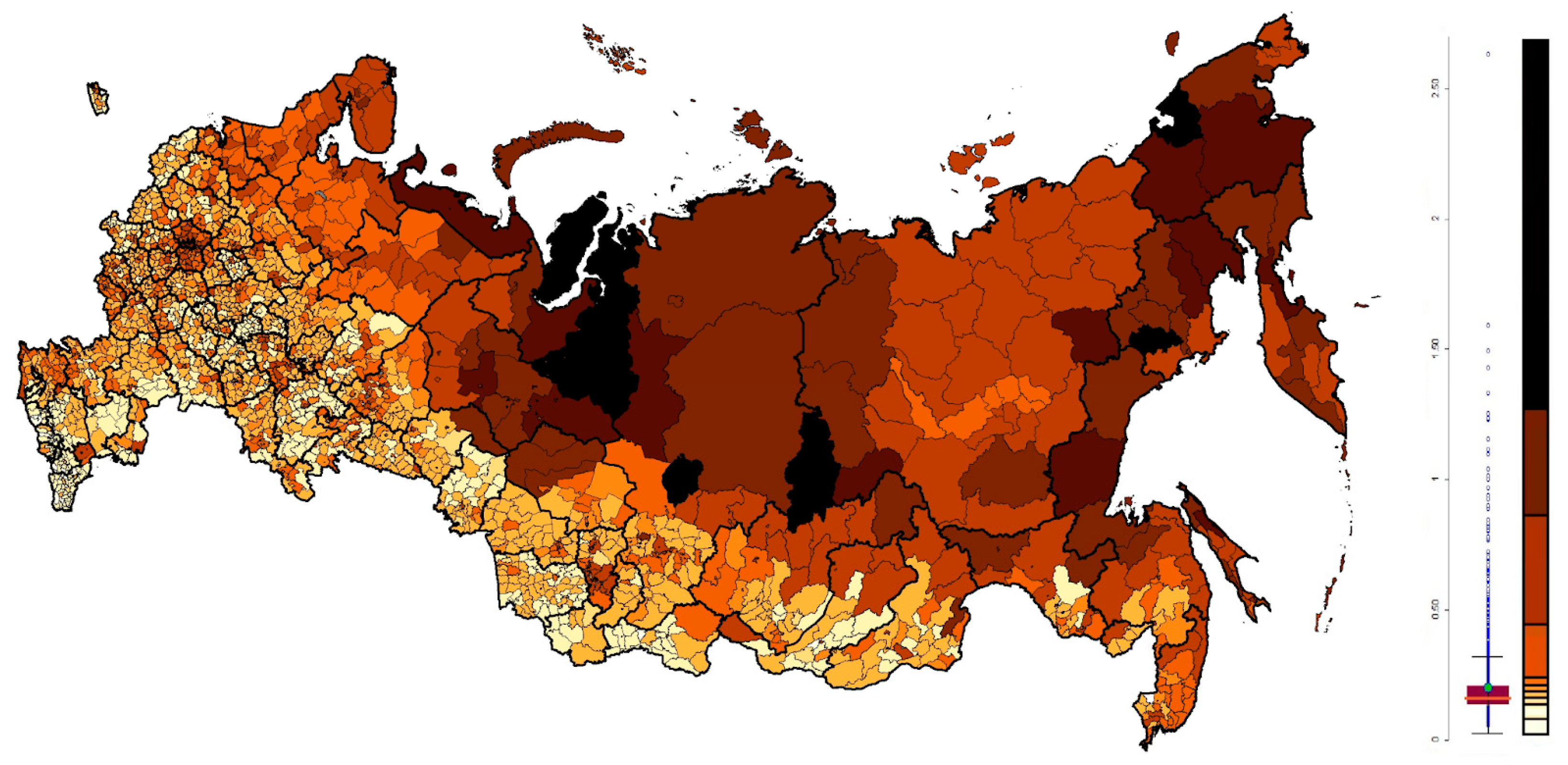
Our research considers two main indicators characterising the population income: volume of social transfers and taxable income (
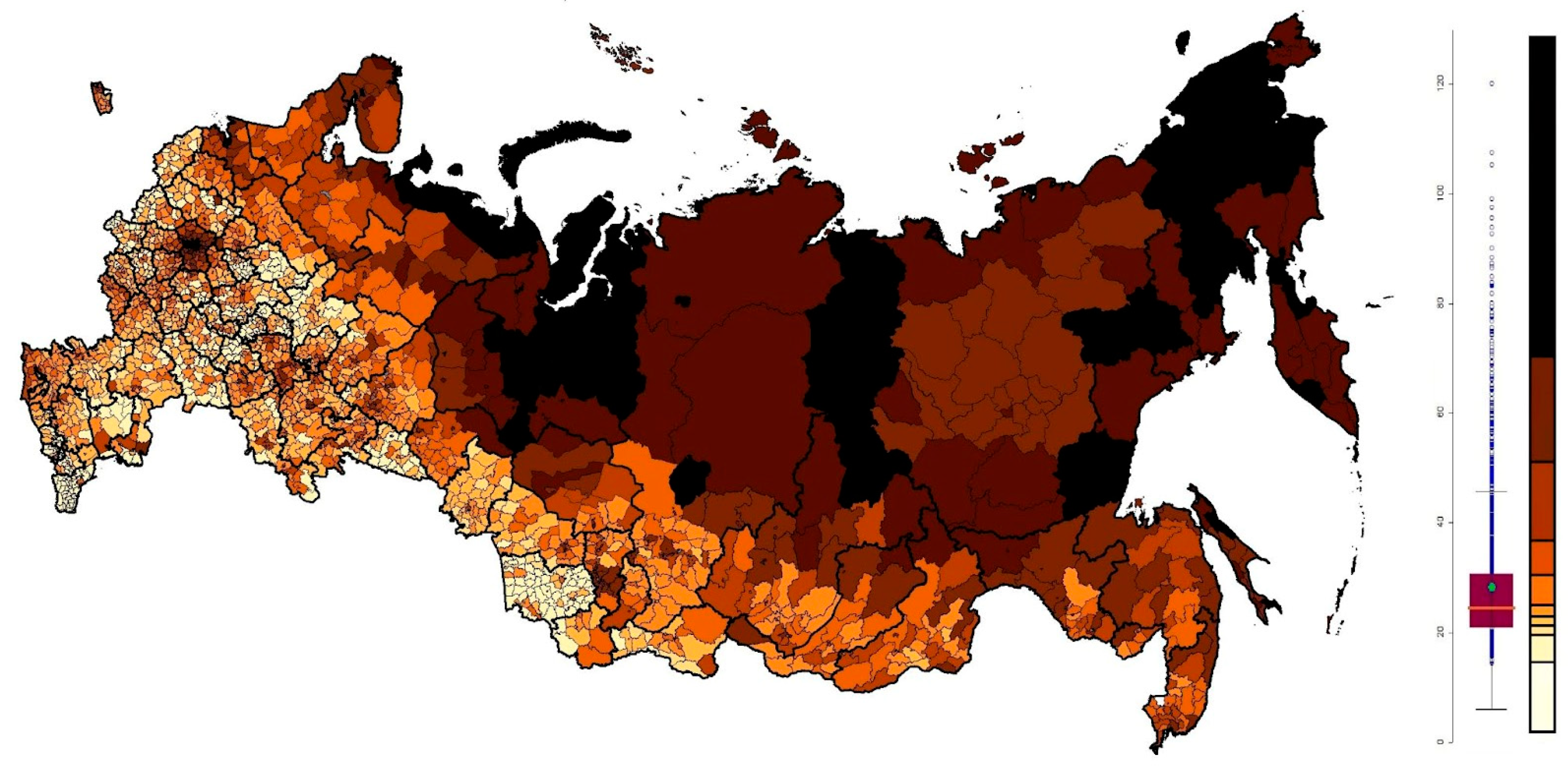
Figure 2) and average nominal employees’ wages of large, medium-sized and non-profit enterprises (
Figure 3).
The variance of social transfers and population taxable income per capita (variable Income per capita) is steadily increasing under the examined period, whereas it remains higher than the variance of average nominal employees’ wages (variable Average wages) which has a downward trend (
Table 1). The largest differences were in 2018. The gap between the lowest and highest municipalities’ peaks of income per capita in 2018 was 64 times (3.22/0.05), while in terms of average wages, it was 8 times (128.84/15.32).
It is worth noting that significant regional differences are combined with a high proportion of municipalities with low population incomes. As a result, we deal with non-normally distributed data that is confirmed by the Shapiro–Wilk normality test. Non-normal data are often found in economic and social studies [
40,
63,
64,
65,
66]. Previous research shows that multilevel models can be resistant to some violations of normality [
66]. The effectiveness of statistical methods when the data distribution is non-normal can be noticeably worse if the type of non-normality is not the same in different groups [
67]. However, in our study, the type of non-normality is the same for all regions: there is an administrative centre with relatively high population incomes and numerous areas with low population incomes.
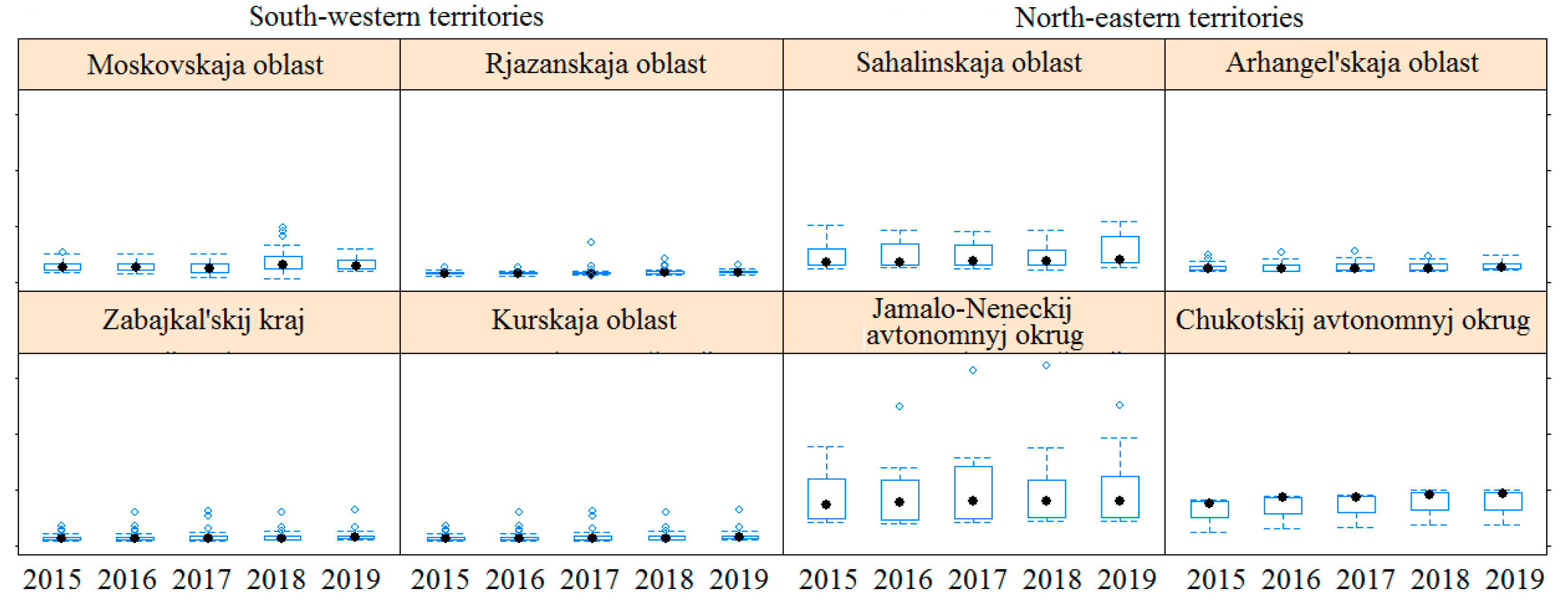
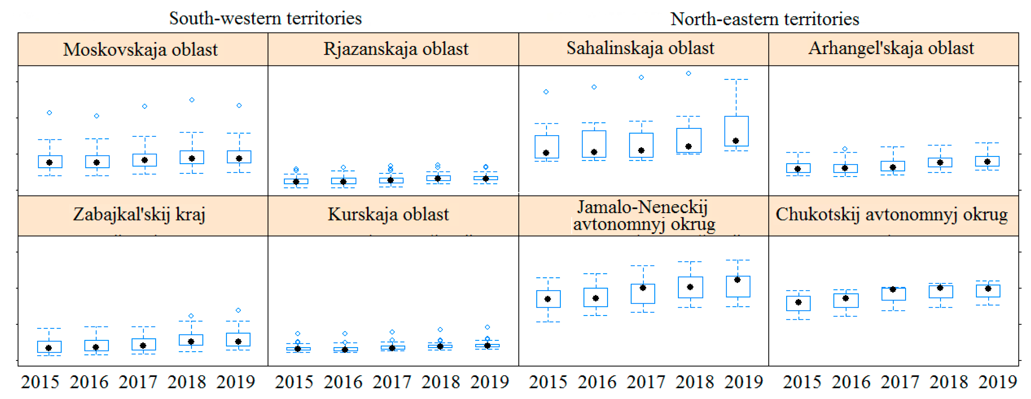
Significant differences between municipalities’ average wages and population income are also found across the regions (
Figure 4 and
Figure 5).
The box plot shows data distribution over time. Observations beyond the «whiskers» are outliers. For some regions, outliers remained during the entire examined period.
The high spread of population income is observed in the northern and north-eastern regions of the country. The low variance of population income is typical for the south-western territories at the municipal scale.
Levin’s and Fligner-Killeen’s tests allow for rejecting the null hypothesis of the same variance among the groups (
Table 2). The tests show that the differences within years are less pronounced than the interregional differences.
Revealed interregional differences indicate the advisability of using multilevel analysis.
4.2. Model of Population Income
Table 3 contains modelling results. The null model (model 1i) is a baseline for comparison of further models; it allows assessment of each level’s contribution to the total variance. Having analysed within- and between-group variance, we found that 23.7% of total variance was associated with municipalities’ differences while 71.9% of total variance was related to differences between regions. Only 0.3% of the total variance was attributed to year differences.
Intra-unit correlation coefficient (IUCC) showed that municipal and regional levels explained 95.9% of the total variance in our data. With adding new predictors into the null model, the random effects in three subsequent models decreased by the part which was explained by enrolled predictors.
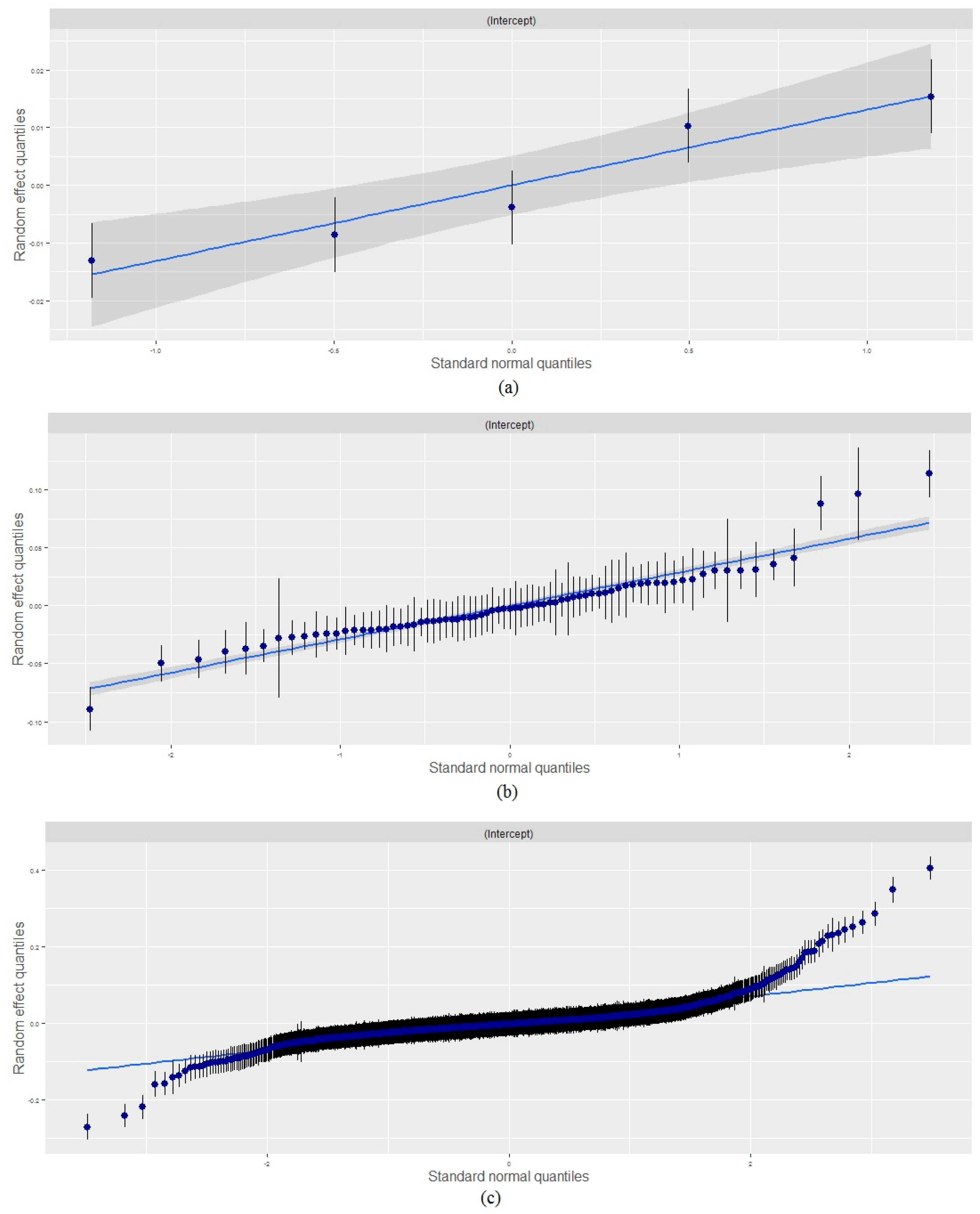
Figure A2 displays model 4i with random effects for every year, region and municipality.
Comparisons of the logarithm of likelihood, Akaike information criteria (AIC), Schwartz (BIC), and deviations (DIC) indicated that each subsequent model was statistically better than the previous one.
Our findings showed that a set of municipal-level factors positively affected population income per capita. Thus, higher population income was observed in municipalities which had a high ratio of working population to population size (Working population per capita). Population size had a positive effect on income per capita, which indicated the positive contribution of population concentration and agglomeration effects. We revealed a positive relationship between production per capita and population income. Moreover, spatial dependency existed. High values of average per capita income in municipalities were positively associated with income in neighbouring territories.
Factors at the regional level had multidirectional influence. In particular, in municipalities with a higher share of agriculture (EmpAgriculture), the population income was lower. Population income was higher in regions with a high share of the extractive industry (EmpMining). The share of employees in the other industries did not have a significant impact on income per capita, while the number of entrepreneurs per capita (Entrepreneurship) had a positive impact.
The relationship between human capital and population income per capita was ambiguous. Only the proportion of employees with secondary vocational education was significant at the p < 0.1 level. This educational level involves the acquisition of working professions (mechanics, builders, drillers, hairdressers, etc.). The rest of the indicators characterising human capital showed insignificance. This indirectly suggested that the drivers of income growth were working professions.
A positive relationship emerged between income per capita, the proportion of working women (Female) and patents registration per capita (Patent). Patenting activity in the region was positively associated with income per capita. At the same time, cross interaction estimate (Production per capita *Patent, γ31jt) had a positive effect on income per capita (model 4i). Cross-interaction estimates showed that factors attributed to the regional level (Patent) determined the relationship between dependent variables (Income per capita) at the municipal level and predictors (Production per capita).
Similarly, cross-interaction estimates demonstrated complex dependencies for indicators of inequality (Gini) and share transfers in population income (Transfers). To explore them in model 4i, we considered the relationship between income per capita and production volume as a function upon which the slope of regression was determined by β coefficient depending on regional predictors: β3ijt = 43.59 + 3.625 * Patent − 2.166 * Transfers.
The obtained coefficients for variables Patent and Transfers indicated the following:
- -
A high volume of production was associated with high volume of income per capita (γ30jt = 43.59);
- -
This relationship would be stronger in regions with a higher share of patent activity (γ31jt = +3.625);
- -
This relationship would be weaker in regions with a higher share of transfers (γ32jt = −2.166).
Constructed model 4i showed mixed manifestations of dependencies across regions.
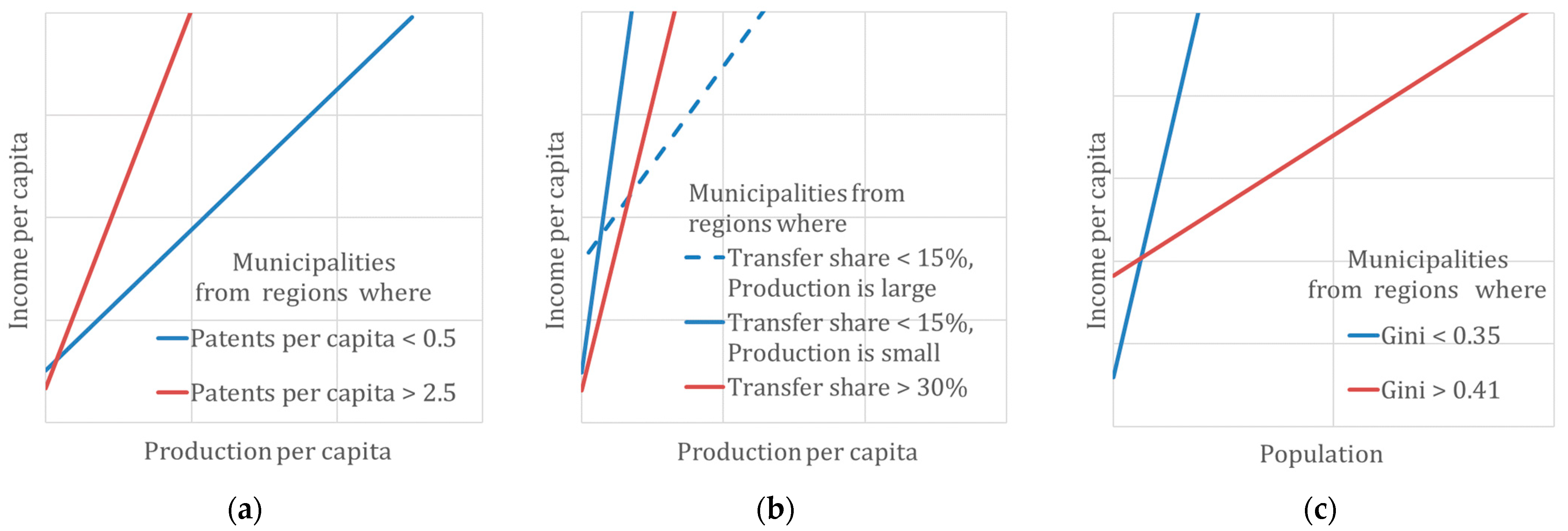
To clearly demonstrate them, we chose municipalities in regions where the number of patents per capita was from 0.5 to 2.5. For each of these groups, we built linear regressions (
Figure 6a). The blue regression line reflects the relationship between income per capita and production volume in regions where the number of granted patents per 10,000 people is below 0.5. The red regression line shows the interconnectedness between income per capita and production volume in regions where the number of granted patents per 10,000 people is more than 2.5. For municipalities attributed to regions that have a larger number of granted patents per 10,000 people, the same production volume is associated with higher population income.
The relationships between the share of transfers in population income, production volume and income per capita are much more complicated.
Figure 6b shows that regions that have a low share of transfers in population income embrace municipalities with high and low production volumes. There, we could distinguish two different dependencies. Regions with a high share of transfers do not include municipalities that have high production volumes per capita.
The multilevel analysis deals with these regional differences.
Figure A1 contains predicted values of income per capita on interaction terms, where other factors are fixed. It also displays differences in marginal effects of interaction terms in model 4i related to various regions.
The dependencies between population size, income per capita and regional Gini coefficient are mixed. In general, inequality is a common characteristic of densely inhabited municipalities while spacely populated regions with low Gini coefficient, growth in population will contribute to increasing income per capita.
4.3. Wage Model
The wage is a part of the population income which people receive for their work and services. Analysis of the total variance showed that 16.2% of average wage variance was attributed to municipalities, 80.8% of it accounted for differences between regions and 1.8% of average wage variance was associated with differences by periods.
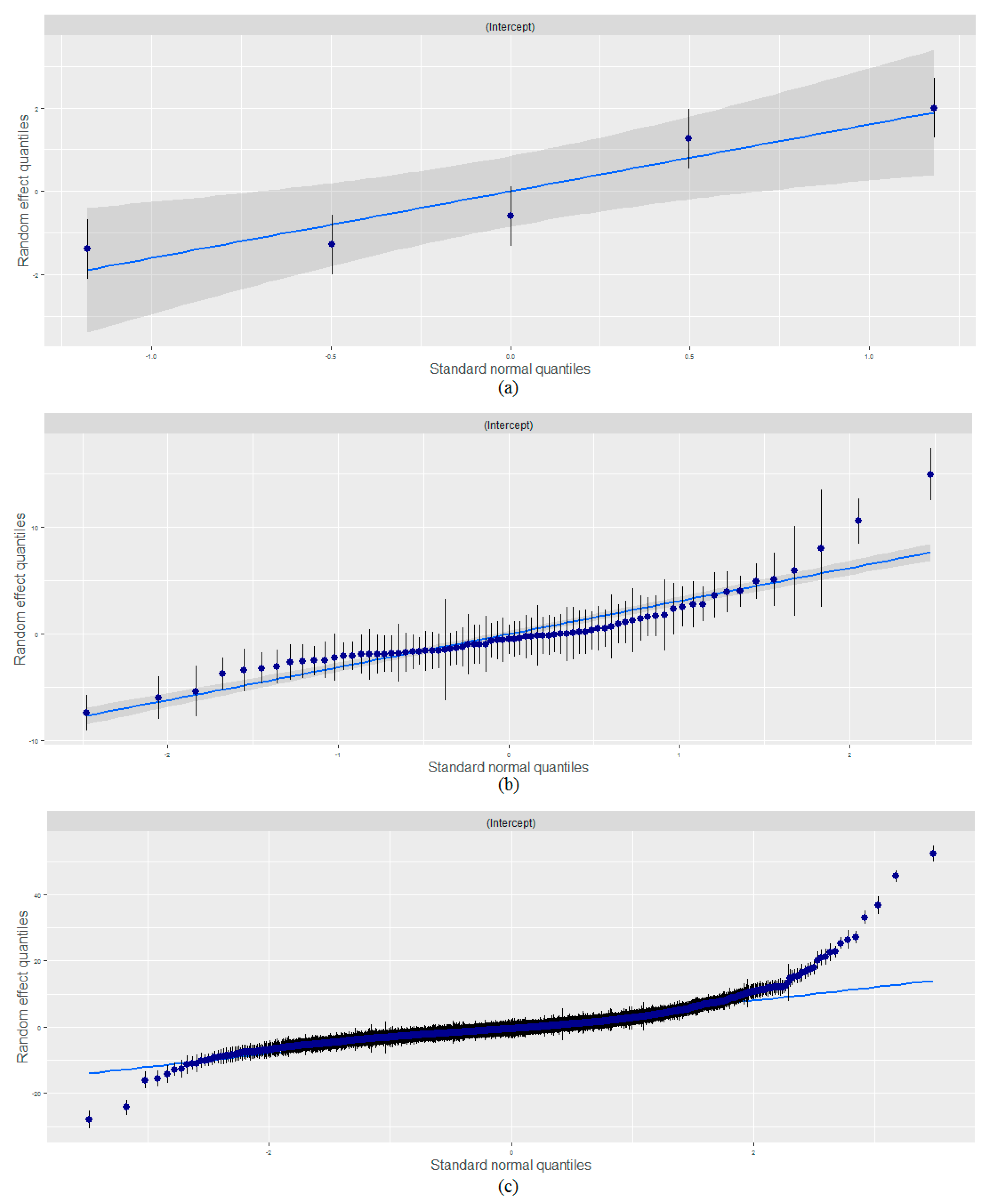
Figure A3 displays model 4w with random effects for every year, region and municipality.
Model 2w embraced factors only at the municipal level (
Table 4) that had a positive effect on the dependent variable. Similar to the model of average per capita income (models 2i, 3i, 4i), the number of the working population had a positive impact on the wage. In contrast to the per capita income model, the wage model took into account the production volume not per capita but per employee, as that was more consistent with productivity. The high productivity complied with the high wage, which was characteristic of municipalities with a high percentage of the urban population.
Wages in municipalities were positively associated with wages in neighbouring municipalities, while unemployment in surrounding regions had no impact on them.
The following factors at the regional scale were not significant in model 3w: the share of employees in manufacturing (EmpManufacturing), the share of employees in catering and hotels (EmpCateringHotels); entrepreneurial activity (Entrepreneurship); the share of the employed population with secondary education (College education); patenting activity (Patent); percentage of employees under 20 years of age (Younger); hazardous working conditions (Harmful), and market potential (WGRP).
Unemployment rate, share of agriculture (EmpAgriculture) and share of transfers in population income (Transfers) are significant at the level p = 0.1 (model 3w). The latter two factors (EmpAgriculture and Transfers) became more significant after adding inter-level interaction in model 4w.
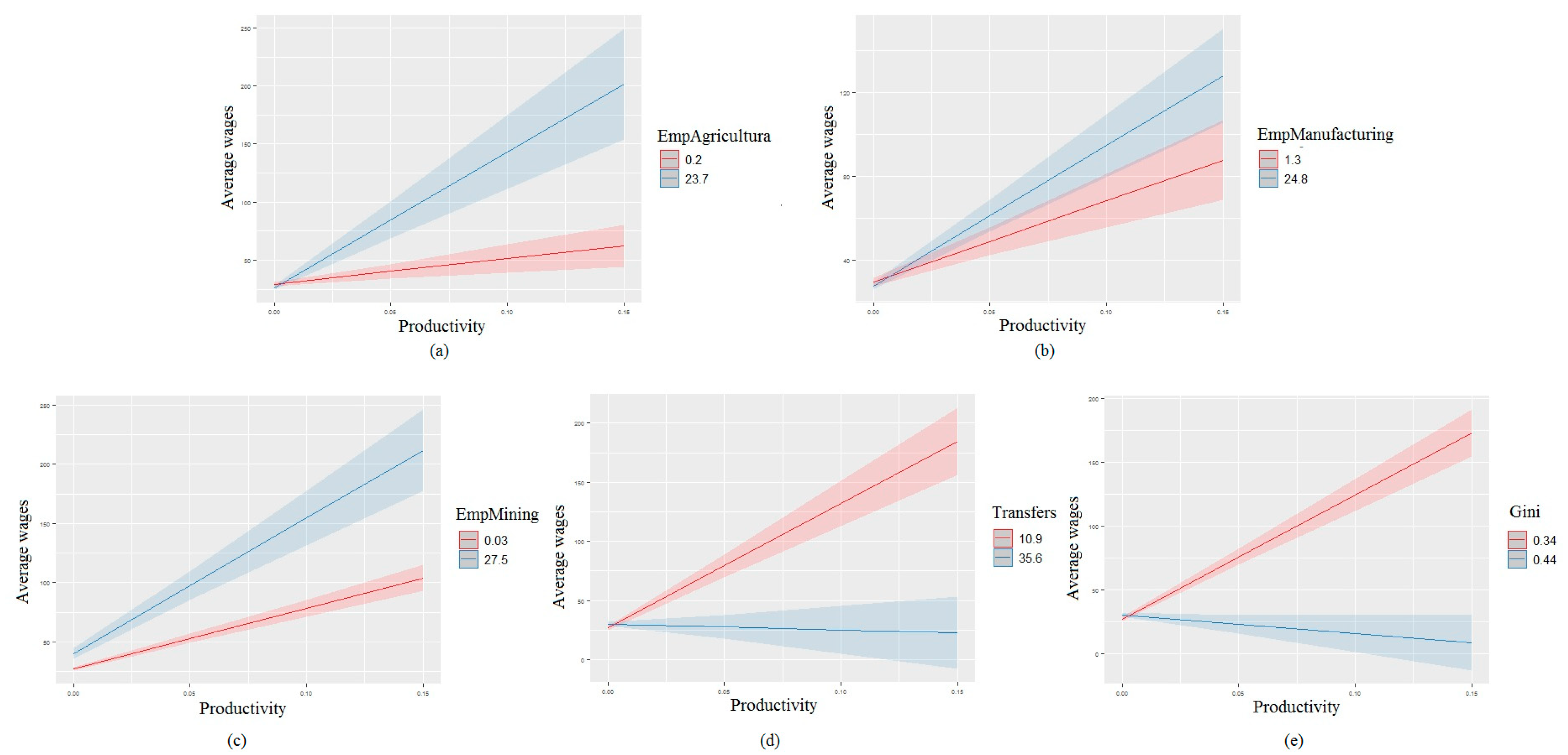
After introducing inter-level interaction into model 4w, p-values improved for many factors, which pointed to the increased statistical quality of the model. We revealed that the relationships between labour productivity and wages were mixed in regions with different economic structures. The high shares of employees in agriculture and mining had a negative impact on the average wage. However, these factors had a positive impact on the relationship between labour productivity and wages. In general, labour productivity growth in these industries had a positive impact on average wages, while the increase in the share of employees had a negative effect. Similarly, the multidirectional influence was also observed for indicators related to income inequality.
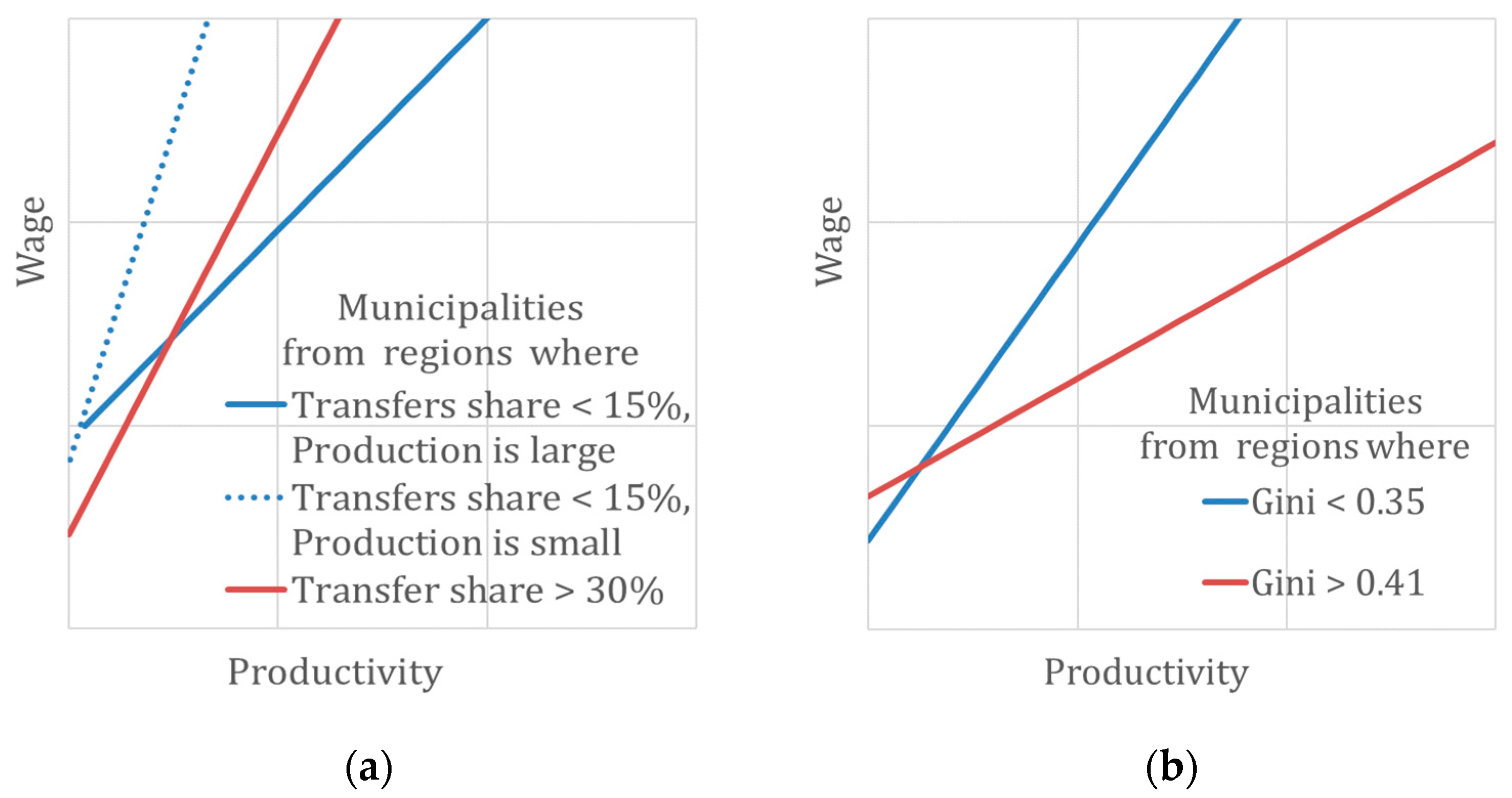
The high value of the Gini coefficient and the share of transfers in the population income had a positive impact on the average wage. The higher the inequality and the more transfers are given, the higher the average wage. However, in regions with high values of these indicators, the relationship between labour productivity and average wages decreases. These dependencies are displayed in
Figure 7, where we highlight municipalities located in regions with high and low values of the Gini coefficient and the share of transfers in population income. This dependence is also observed when calculating the effects for average wages model 4w, where other factors are fixed (
Figure A4).
A comparison of the logarithm of likelihood, Akaike information criteria (AIC), Schwartz (BIC) and deviations (DIC) indicates that each subsequent model is better than the previous one. Thus, model 4w takes into account the inter-level interactions and better explains the observed interregional and intraregional wage differences.
5. Discussion
Our research underlines once again that each country has its own characteristics determining the uneven income distribution. Our study shows that in Russia, 23.7% of the total variance of per capita income is associated with municipalities (intraregional differences), and 71.9% of it is attributed to differences between regions. Regions contribute more to the heterogeneity of wages: 80.8% of the total variance accounts for regions, i.e. it manifests itself at the upper level of administrative-territorial division. Studies conducted on data from other countries showed that the lower level of the hierarchy had a much greater influence on indicators under consideration [
42].
This situation is largely due to the significant climatic differences between the north and south and the sectoral differences between the regions determined by the endowment of natural resources [
31,
32,
36]. Against the background of significant interregional differences, intraregional ones are not so strong. Income variance is higher and tends to increase while wage variance is declining. Population income embraces wages, social transfers, entrepreneurial incomes and property incomes. Our empirical results show that a number of factors have different impacts on population income and wage. Population income and wages are strongly dependent on the structure of the economy. The high share of employees in agriculture (EmpAgriculture) in the economy is negatively associated with these variables, while the high share of employees in mining (EmpMining) has a positive impact on them. Revealed relationships are common for many countries [
12,
16,
55,
56,
68], including Russia [
24]. The development of the other industries did not influence the population income per capita, whereas we found additional effects related to wages. In line with Demidova and Timofeeva [
24], the share of employees in construction had a positive effect on the average wage in municipalities. The share of employees in manufacturing (EmpManufacturing) had a mixed impact. On the one hand, it negatively affected the average wage. This situation was similar to Stansel [
17], who found a negative relationship between manufacturing share and growth in the log of real per capita money income. Breau [
9] revealed negative interconnectedness between the labour force employed in manufacturing and inequality, which was examined using employment earnings. Demidova and Timofeeva [
24] pointed out the same negative relationship in exploring wages in Russia. On the other hand, our calculations showed that Manufacturing had a positive effect on the relationship between labour productivity and wages. It could be explained by lower wages in Manufacturing than in other industries (for example, Mining). However, we observed higher wages in manufacturing industries in regions with high labour productivity. Thus, we clarified that manufacturing share was not so important itself, but the labour productivity in this industry. Baddeley et al. [
19] identified that manufacturing employment had a different impact on regional wages in Europe and USA. The number of individual entrepreneurs per capita (Entrepreneurship) had a positive impact on the population’s income, and it was insignificant for the average wage. This finding could be explained by the inclusion of entrepreneurial income in population income. The more people gain entrepreneurial income, the higher the population income. The nonsignificant relationship between entrepreneurial income and population income might be due to the low share of the entrepreneurship sector in the country’s economy. At the same time, the ratio of the average number of employees of small and medium-sized enterprises to the total population (variable EmpSmallBusiness) was negatively associated with average wages, which supported previous studies [
24,
55].
Working population per capita had a positive impact on both average wage and population income. The variable Working population per capita had regional features, one of which was severe climatic conditions that made northern areas sparsely populated, causing the engagement of a labour force from the other regions for extractive activities. In a number of municipalities, the number of employees of organisations is 2.5 times more than the number of permanent inhabitants. The south regions are attractive to retirees. There are other labour flows circulating within regions. Huge cities absorb many employees while the unemployed adult population is located in surrounding areas, which feature a small share of the working population per capita and a large share of the population receiving social transfers. Our study shows that the average wage and income per capita are higher in municipalities with a high share of the working population. This result is consistent with previous research, which highlights that higher labour force ratio leads to a lower poverty incidence [
5]. At the same time, the unemployment rate variable shows a low significance. In our view, our study does not contradict previous studies in which unemployment is closely associated with wages [
20,
24,
53,
54,
55]. The structure of the data must be taken into account. We included the variable of unemployment at the regional level because these estimates were missed at the municipal scale. At the regional level, they poorly account for unemployment in the cities and villages, in the centre and the periphery generalising the assessment. We took the variable of working population per capita as an indirect measure of unemployment in municipalities which showed a significant impact on population income because it took into account the characteristics of each municipal labour market.
Thus, the insignificance of the unemployment rate in the model did not arise from its weak connection with wages; it was a consequence of the unemployment indicator aggregated at the regional scale without consideration of municipal characteristics. To gain a better understanding of intraregional (urban–rural, core–periphery) patterns of disparities, we included variables of population distribution within regions. Our findings revealed that population concentration positively affected income per capita; Stansel [
17] found the same relationship. The share of the urban population is an essential factor of urban–rural income disparity [
24,
58]. Our study confirmed its significant positive impact on wages. Our study disclosed the significance of such spatial factors as the proximity of regions. Two models showed that population income in certain regions had a direct relationship with the population income in neighbouring regions. Thus, the growth of incomes and wages in one region will have an impact on their growth in neighbouring regions.
The quality and structure of labour determine wages [
9,
17,
18,
48,
52]. The educational level is one of the essential factors influencing inequality in the level and rate of income growth. Recent developments established different relationships between educational level and population income. In particular, a number of studies showed that a bachelor’s degree had a positive effect on the population income in the United States, while a college graduate had a negative effect [
48,
52]. Breau and Saillant [
10] revealed that the percentage of the labour force with a bachelor’s degree or higher did not affect real average total income growth in Canada. Candelaria et al. [
56] showed a positive relationship between the number of college graduates per capita and average real wages. López-Rodríguez and Faíña [
13] established that the share of the economically active population with medium and high educational levels positively affected compensation per employee, defined as the total remuneration in wages and salaries. The number of patents per capita also depends on the level of human capital development [
13]. In our study, the different educational levels positively affected wages and population income. The wage was dependent on a bachelor’s degree and a higher educational level. The income per capita was associated with college degrees and the number of patents per capita. This difference may have several reasons. Population income includes, in addition to the wage, property income, which may be higher for owners actively introducing new technologies in regions with high patent registration. The benefits of higher education (“education pays”) are perceived to influence wages [
23], but our research showed that they might not be reflected in the total income. These assumptions remain highly debatable, requiring a deeper study of the relationship between education and population income. Čadil et al. [
69] suggested that one of the reasons for such a different impact may be unsuitable education. It should be noted that the quality of education may be variable within Russian regions [
70]. As a result, an estimation of the people proportion with a certain level of education without its quality measurement may be insignificant. In our models (3i, 4i), the share of people with higher education is not significant, while the number of registered patents has a significant effect on population income. This actually indicates that the number of people with higher education is not so important as whether they can generate new knowledge and new products.
In addition to benefits of higher education, wages may reflect benefits for speed and memory of younger workers, the work experience of older workers [
23] and hazardous working conditions [
21]. Our study showed that a high proportion of workers over 50 (Older) had a significant negative impact on average wages. Demidova and Timofeeva [
24] gained similar results in their model specifications. This suggests that benefits for work experience are not formed in the labour market. Older people, due to various factors (health status, the value of free time, etc.), are ready to take less-paid jobs. The share of employees working in hazardous conditions is not significant in the model, which is consistent with previous research [
21]. This raises questions on the fairness of pay, which gets scant attention in Russia. In fact, work in hazardous conditions is not compensated by wages. Bockerman and Ilmakunnas [
21] revealed the same relationship. They additionally conducted experiments with alternative definitions of the disamenity variables. They take the coefficient for the HARM as a sum of the adverse job characteristics; it has a positive impact on wages at the 10% significance level [
21]. Despite the weak relationship between work in hazardous conditions and wages in Russia, the government provides early retirement as another type of compensation. Protection of the interests of employees is one of the main tasks of trade unions. Conducted analysis showed a significant and positive impact of trade union activities on the average wage in Russia, while studies in other countries disclosed that trade unions might influence wages [
54] or might not [
19].
The differences in labour productivity are a crucial factor in understanding wage heterogeneity. An important condition for the growth of population income per capita is the growth of production per capita. These close relationships have been the research focus of academics for many years [
5,
20,
26,
53,
54]. Inequality and mechanisms of government regulation of population income and wages are also actively studied [
9,
16,
28,
38,
48,
52,
56]. Russian scientists also found a strong positive correlation between population income and inequality in most regions, but some of them did not demonstrate this interconnectedness [
22].
Many studies underlined the controversial relationship between income inequality and population income per capita [
16,
48,
52]. Our study aimed to address the problem comprehensively; it showed that the government could directly influence the growth of income and implicitly affect the relationship between population income and productivity.
We took the Gini coefficient as the measure of inequality in income distribution; it had a direct effect on the dependent variable in both models. Thus, inequality growth led to an increase in average wage and population income through the income rise of the richest. The increase in social transfers also contributed to the growth of population income. At the same time, we established a direct impact of transfers on the average wage. To attract workers, the employer should provide wages higher than the social transfers that a person could get without work. Our calculations also showed an indirect effect. The relationship between labour productivity and wages manifests itself differently in regions with high- and low-income inequality and in regions with a high and low share of the social transfers. An increase in labour productivity in regions with a higher Gini coefficient will have less impact on wages than in regions with a low Gini coefficient.
The impact of social transfers is more complex and additionally determined by the size of economies. Since social transfers are usually allocated to the least developed regions, it is reasonable to compare regions with a high share of transfers and regions with a weak economy but a low share of transfers in the population income.
For both income per capita and average wage, productivity gains in regions with a high share of transfers led to lower growth of income than in regions with a low share of transfers. These results confirmed a complex and contradictory relationship between population income, inequality and government support measures which could have an ambiguous impact [
16,
48,
52].
Our findings are in line with previous studies that revealed a contradiction between real economies and the neo-classical paradigm, which suggests that in a market economy, regional income disparities should be eliminated through labour mobility, trade, etc. [
56]. In transitional Russia, laws of neoclassical economics were not implemented. Thus, further studies aimed at exploring regional contexts are becoming important. We found that income inequality differed from wage inequality while the influence of social transfers on them was mixed. Our findings are similar to Blundell et al. [
30]. We revealed different wage and population income trends reflecting volatile wage share in population income and regional specifics. Regional wage disparities were declining while inequalities in population income were rising. Thus, the other components of population income changed in structure and contributed to this gap and increase in regional inequalities over time. This explains the importance of further research on variances of population income and wage in the heterogeneous economic system of Russia.
6. Conclusions
Our study contributes to a growing body of literature on population income inequality patterns at regional and municipal scales. We used data on 2017 municipalities across 75 from 85 Russian regions. We took population income and average wage as dependent variables; the data set covers the period from 2017 to 2019. Our paper aimed to provide a deeper study of population income inequality, emphasising interregional and intraregional factors within the framework of multilevel models. Our findings showed that differences between regions had the greatest influence (71.9% for income per capita and 80.8% for an average wage). Only 0.3% of the total variance is attributed to year differences. Thus, intra-regional differences are not as great as inter-regional ones, which differs from the ratios for other countries. The variance of income per capita is steadily increasing under the examined period, whereas it remains higher than the variance of average employees’ wages which has a downward trend. Multilevel models allow separate consideration of factors at municipal and regional scales, which determine these disparities.
The modelling results showed that income per capita and average wage were positively associated with such factors at the municipal scale as working population per capita and production per capita. The concentration of population had a positive effect on income per capita; the relationship between the share of the urban population and the average wage was positive. Moreover, we revealed spatial dependencies of indicators. We found direct positive relationships between (a) income per capita and income per capita in neighbouring municipalities; (b) average wage and the average wage in neighbouring municipalities.
The share of employees in the mining industry (variable EmpMining), women’s participation in the labour force, Gini coefficient and transfers had both a positive impact on income per capita and average wage. However, a high share of employees in agriculture and fishing was negatively associated with dependent variables. These dependencies were established previously, but our study had an important addition to existing studies.
We quantified the negative impact of income inequality and a policy of high social transfers on the relationship between labour productivity and dependent variables (income per capita and average wage), including cross-level interactions in the model. We also showed that a high share of employees in agriculture and in manufacturing, despite a direct negative impact on the average wage, enhanced the role of labour productivity in wage formation.
Another important result of the study was uncovering the reasons behind different variances in population income per capita and the average wage. At the regional level, we revealed that the number of entrepreneurs per capita, the share of the employed population with secondary education (variable College education) and the volume of patents granted for inventions and utility models per 10,000 population had a positive impact on the population income per capita.
At the same time, the share of employees in the construction industry, the share of the employed population with high education, the activity of trade unions and exports are positively associated with average wage while the share of employees in manufacturing, the average number of employees of small and medium-sized enterprises to the population and employees over 50 years had a negative impact on the average wage. Thus, the factors that influence wages and total income are different.
Our paper is one of the few studies considering the problem of income inequality in Russia with data of such magnitude. However, our study is not without shortcomings. Firstly, we study the total population income without close examination of differences in property income and conditions of their formation. Secondly, we measured income inequality only through the Gini index, and further studies should include the individual as the additional level of the hierarchy. This will allow us to take a close look at the personal skills determining inequality and reveal the role of education that showed mixed results. Thirdly, examined data have non-normal distribution. This is a common problem for many socio-economic processes, and the performance of different methods under non-normality for multilevel designs is being widely discussed [
40,
63,
64,
65,
66,
67]. Thus, the results should be treated with caution. Fourthly, the current state of the Russian economy in light of recent events is unstable. Thus, the significance of our study is currently determined not so much by the assessment of inequality in the period 2017–2019 but by highlighting the variety of unevenness forms and determining the possibilities of multilevel modelling in their analysis.
Our study on population income inequality is insightful because it allows disclosing the causes and separating the influence of factors at the regional and municipal levels, which corresponds to the hierarchy of administrative-territorial demarcation.
The use of cross-level interactions within the framework of a hierarchical (multilevel) model made it possible to illuminate the importance of the regional context for the development of municipalities and establish why in some regions, certain factors have a greater impact on population income than in others. Therefore, a universal approach to the development of regional policy cannot be efficient due to the existence of various factors in the regions. Given these constraints, we attempted to show the advantages of this method in exploring regional peculiarities for making spatial decisions.

