Analytic Error Function and Numeric Inverse Obtained by Geometric Means

Abstract

Using geometric considerations, we provided a clear derivation of the integral representation for the error function, known as the Craig formula. We calculated the corresponding power series expansion and proved the convergence. The same geometric means finally assisted in systematically deriving useful formulas that approximated the inverse error function. Our approach could be used for applications in high-speed Monte Carlo simulations, where this function is used extensively.

1. Introduction

High-speed Monte Carlo simulations are used for across a broad spectrum of applications, from mathematics to economics. As input for such simulations, the probability distributions are usually generated by pseudo-random number sampling, a method derived from the work of John von Neumann in 1951 [1]. In the era of “big data”, such methods have to be fast and reliable, and a sign of this necessity was the release of Quside’s inaugural processing unit in 2023 [2]. However, these samplings need to be cross-validated by exact methods, and for this, the knowledge of analytical functions that describe the stochastic processes, and among those, the error function, are of tremendous importance.

By definition, a function is called analytic if it is locally given by a converging Taylor series expansion. Even if a function itself is not found to be analytic, its inverse could be analytic. The error function could be given analytically, and one of these analytic expressions was the integral representation found by Craig in 1991 [3]. Craig mentioned this representation only briefly and did not provide a derivation of it. Since then, there have been a couple of derivations of this formula [4,5,6]. In Section 2, we describe an additional one that is based on the same geometric considerations as employed in [7]. In Section 3, we provide the series expansion for Craig’s integral representation and show the rapid convergence of this series.

For the inverse error function, the guidance for special functions (e.g., [8]) do not unveil such an analytic property. Instead, this function has to be approximated. Known approximations date back to the late 1960s and early 1970s [9,10]) and include semi-analytical approximations by asymptotic expansion (e.g., [11,12,13,14,15,16]. Using the same geometric considerations, as shown in Section 4, we developed a couple of useful approximations that can easily be implemented in different computer languages, resulting in the deviations from an exact treatment. In Section 5, we discuss our results and evaluate the CPU time. Section 6 contains our conclusions.

2. Derivation of Craig’s Integral Representation

The authors of [7] provided an approximation for the integral over the Gaussian standard normal distribution that is obtained by geometric considerations and is related to the cumulative distribution function via $P\left(t\right)=\Phi \left(t\right)-\Phi (-t)$, where $\Phi \left(t\right)$ is the Laplace function. The same considerations apply to the error function $\mathrm{erf}\left(t\right)$ that is related to $P\left(t\right)$ via

$$\mathrm{erf}\left(t\right)=\frac{1}{\sqrt{\pi }}{\int }_{-t}^t{e}^{-x^2}dx=\frac{1}{\sqrt{2\pi }}{\int }_{-\sqrt{2}t}^{\sqrt{2}t}{e}^{-x^2/2}dx=P\left(\sqrt{2}t\right).$$

(1)

Translating the results of [7] into the error function, we obtained the approximation of order p by the following:

$${\mathrm{erf}}_p{\left(t\right)}^2=1-\frac{1}{N}\sum _{n=1}^N{e}^{-k_{p,n}^2{t}^2},$$

(2)

where the $N=2^p$ values $k_{p,n}$ ($n=1,2,\dots ,N$) are found in the intervals between $1/cos\left(\pi \right(n-1)/(4N\left)\right)$ and $1/cos(\pi n/(4N\left)\right)$. A method for selecting those values was extensively described in [7], where the authors showed the following:

$$|\mathrm{erf}\left(t\right)-\sqrt{1-e^{-k_{0,1}^2{t}^2}}|<0.0033$$

(3)

for $k_{0,1}=1.116$. With $14\approx 0.0033/0.00024$ times larger precision, the following was expressed:

$$|\mathrm{erf}\left(t\right)-\sqrt{1-\frac{1}{2}(e^{-k_{1,1}^2{t}^2}+e^{-k_{1,2}^2{t}^2})}|<0.00024,$$

(4)

for $k_{1,1}=1.01$ and $k_{1,2}=1.23345$. For the parameters $k_{p,n}=1/cos(\pi n/\left(4N\right))$ of the upper limits of those intervals, we calculated the deviation by the following:

$$|\mathrm{erf}\left(t\right)-{\mathrm{erf}}_p\left(t\right)|<\frac{exp(-t^2)}{2N}\sqrt{1-exp(-t^2)}.$$

(5)

Given the values $k_{p,n}=1/cos\varphi \left(n\right)$ with $\varphi \left(n\right)=\pi n/\left(4N\right)$, with the limit $N\to \infty$, the sum over n in Equation (2) could be replaced by an integral with measure $dn=(4N/\pi )d\varphi \left(n\right)$ to obtain the following:

$$\mathrm{erf}{\left(t\right)}^2=1-\frac{4}{\pi }{\int }_0^{\pi /4}exp\left(\frac{-t^2}{{cos}^2\varphi }\right)d\varphi .$$

(6)

3. Power Series Expansion

The integral in Equation (6) could be expanded into a power series in $t^2$,

$$\mathrm{erf}{\left(t\right)}^2=1-\frac{4}{\pi }\sum _{n=0}^{\infty }{c}_n\frac{{(-1)}^n}{n!}{\left(t^2\right)}^n$$

(7)

with

$$\begin{array}{ccc}{c}_n\hfill & =& {\int }_0^{\pi /4}\frac{d\varphi }{{cos}^{2n}\varphi }={\int }_0^{\pi /4}{(1+{tan}^2\varphi )}^{n}d\varphi ={\int }_0^1{(1+y^2)}^{n-1}dy\hfill \\ & =& \sum _{k=0}^{n-1}\left(\begin{array}{c}n-1\\ k\end{array}\right){\int }_0^1{y}^{2k}dy=\sum _{k=0}^{n-1}\frac{1}{2k+1}\left(\begin{array}{c}n-1\\ k\end{array}\right),\hfill \end{array}$$

(8)

where $y=tan\varphi$. The coefficients $c_n$ could be expressed by the hyper-geometric function, $c_n={}_2{F}_1(1/2,1-n;3/2;-1)$, also known as Barnes’ extended hyper-geometric function. However, we could derive a constraint for the explicit finite series expression for $c_n$ that rendered the series in Equation (7) convergent for all values of t. In order to be self-contained, the intermediate steps to derive this constraint and to show the convergence were shown by the following, in which the sum over the rows of Pascal’s triangle was required:

$$\sum _{k=0}^n\left(\begin{array}{c}n\\ k\end{array}\right)=2^n.$$

Returning to Equation (8), we had $0\le k\le n-1$. Therefore,

$$\frac{1}{2n-1}\le \frac{1}{2k+1}\le 1.$$

The result in Equation (8) led to the following:

$$\frac{1}{2n-1}\sum _{k=0}^{n-1}\left(\begin{array}{c}n-1\\ k\end{array}\right)\le c_n\le \sum _{k=0}^{n-1}\left(\begin{array}{c}n-1\\ k\end{array}\right)=2^{n-1},$$

where the existence of a real number $c_n^{\ast }$ is between $1/(2n-1)$ and 1, such that $c_n=c_n^{\ast }{2}^{n-1}$. We found the following:

$${\mathrm{erf}}_p{\left(t\right)}^2=1-\frac{4}{\pi }\sum _{n=0}^N{c}_n\frac{{(-1)}^n}{n!}{\left(t^2\right)}^n=1-\frac{2}{\pi }\sum _{n=0}^N{c}_n^{\ast }\frac{{(-2t^2)}^n}{n!}.$$

Because of $0\le c_n^{\ast }\le 1$, there was again a real number $c_N^{\ast \ast }$ in the corresponding open interval so that the following was true:

$$\frac{2}{\pi }\sum _{n=0}^N{c}_n^{\ast }\frac{{(-2t^2)}^n}{n!}=c_N^{\ast \ast }\frac{2}{\pi }\sum _{n=0}^N\frac{{(-2t^2)}^n}{n!}<\frac{2}{\pi }\sum _{n=0}^N\frac{{(-2t^2)}^n}{n!}.$$

As the latter was the power series expansion of $(2/\pi )e^{-2t^2}$, which was convergent for all values of t, the original series was then also convergent and, thus, ${\mathrm{erf}}_p{\left(t\right)}^2$ with the limiting value shown in Equation (7). A more compact form of the power series expansion was expressed by the following:

$$\mathrm{erf}{\left(t\right)}^2=\sum _{n=1}^{\infty }{c}_n\frac{{(-1)}^{n-1}}{n!}{\left(t^2\right)}^n,c_n=\sum _{k=0}^{n-1}\frac{1}{2k+1}\left(\begin{array}{c}n-1\\ k\end{array}\right).$$

4. Approximations for the Inverse Error Function

Based on the geometric approach described in [7], we were able to describe simple, useful formulas that, when guided by consistently higher orders of the approximation (2) for the error function, led to consistently more advanced approximations of the inverse error function. The starting point was the degree $p=0$, that is, the approximation in Equation (3). Inverting $E={\mathrm{erf}}_0\left(t\right)={(1-e^{-k_{0,1}^2{t}^2})}^{1/2}$ led to $t^2=-ln(1-E^2)/k_{0,1}^2$, and using the parameter $k_{0,1}=1.116$ from Equation (3) yielded the following:

$$T_0=\sqrt{-ln(1-E^2)}/k_{0,1}^2.$$

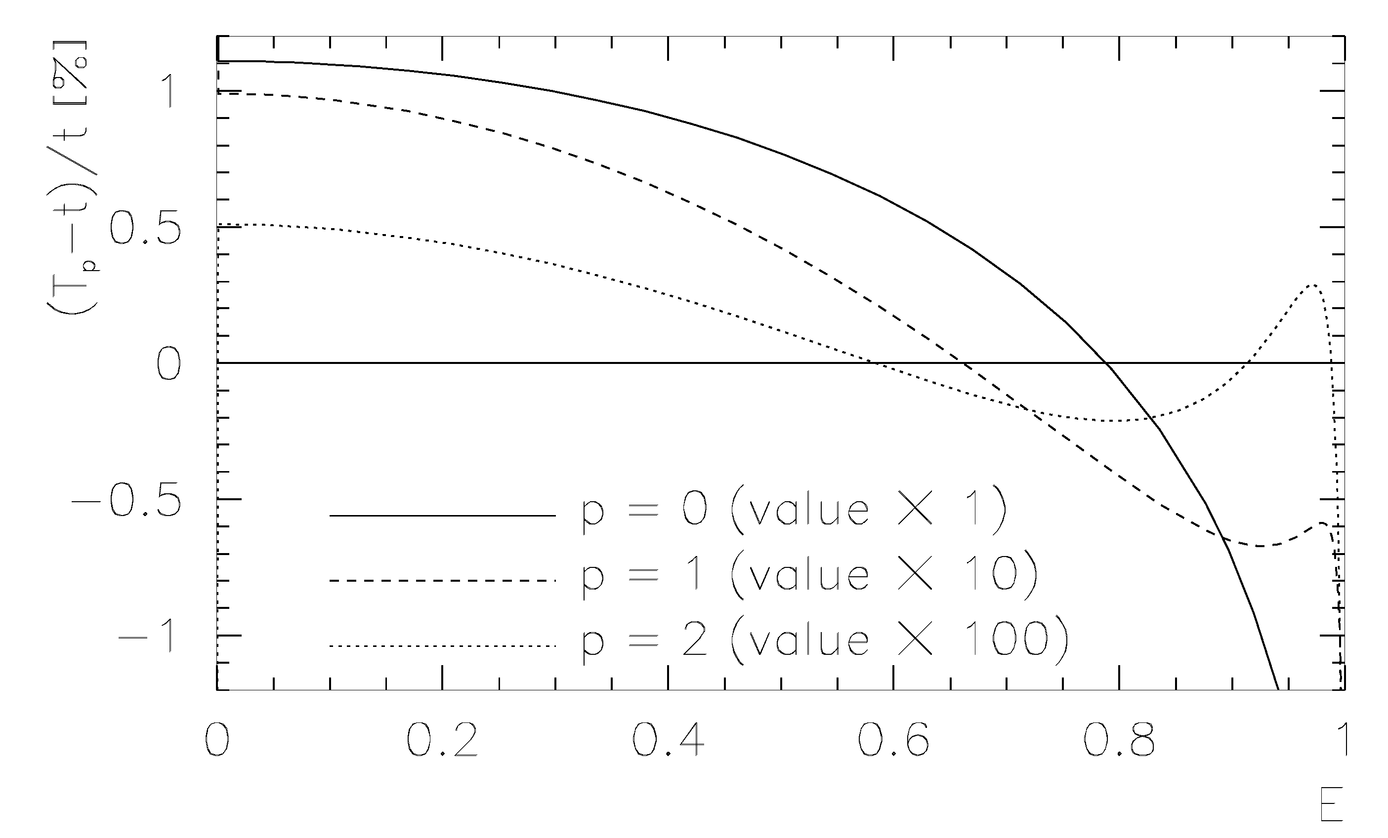
For $0\le E\le 0.92$, the relative deviation $(T_{\left(0\right)}-t)/t$ from the exact value t was less than $1.11\%$, and for $0\le E<1$, the deviation was less than $10\%$. Therefore, for $E>0.92$, a more precise formula has to be used. As such, higher values for E appeared only in $8\%$ of the cases, so this would not significantly influence the CPU demand.

Continuing with $p=1$, we inserted $T_0=\sqrt{-ln(1-E^2)}/k_{0,1}^2$ into Equation (2) to obtain the following:

$${\mathrm{erf}}_1\left(T_0\right)=\sqrt{1-\frac{1}{2}(e^{-k_{1,1}^2{T}_0^2}+e^{-k_{1,2}^2{T}_0^2})},$$

where $k_{1,1}=1.01$ and $k_{1,2}=1.23345$ are the same as for Equation (4). Using the derivative of Equation (1) and approximating this by the difference quotient, we obtained the following:

$$\frac{\mathrm{erf}\left(t\right)-\mathrm{erf}\left(T_0\right)}{t-T_0}=\frac{\Delta \mathrm{erf}\left(t\right)}{\Delta t}{|}_{t=T_0}\approx \frac{d\mathrm{erf}\left(t\right)}{dt}{|}_{t=T_0}=\frac{2}{\sqrt{\pi }}{e}^{-T_0^2},$$

resulting in $t\approx T_1=T_0+\frac{1}{2}\sqrt{\pi }{e}^{T_0^2}(E-{\mathrm{erf}}_1\left(T_0\right))$. In this case, for the larger interval $0\le E\le 0.995$, the relative deviation $(T_1-t)/t$ was less than $0.1\%$. Using ${\mathrm{erf}}_2\left(t\right)$ instead of ${\mathrm{erf}}_1\left(t\right)$ and inserting $T_1$ instead of $T_0$, we obtained $T_2$ with a relative deviation of maximally $0.01\%$ for the same interval. The results are shown in Figure 1.

The method could be optimized by a method similar to the shooting method in boundary problems, which would add dynamics to the calculation. Suppose that following one of the previous methods, for a particular argument E, we found an approximation $t_0$ for the value of the inverse error function of this argument. Using $t_1=1.01t_0$, we could adjust the improved result

$$t=t_0+A(E-\mathrm{erf}\left(t_0\right))$$

by inserting $E=\mathrm{erf}\left(t\right)$ and calculating A for $t=t_1$. In general, this procedure provided a vanishing deviation close to $E=0$. In this case as well as for $t_0=T_1$, in the interval $0\le E\le 0.7$, the maximal deviation was slightly larger than ${10}^{-6}=0.0001\%$, while up to $E=0.92$ the deviation was restricted to ${10}^{-5}=0.001\%$. A more general ansatz

$$t=t_0+A(E-\mathrm{erf}\left(t_0\right))+B{(E-\mathrm{erf}\left(t_0\right))}^2$$

could be adjusted by inserting $E=\mathrm{erf}\left(t\right)$ for $t=1.01t_0$ and $t=1.02t_0$, and yielded the system of equations:

$$\Delta t=A\Delta E_1+B\Delta E_1^2,2\Delta t=A\Delta E_2+B\Delta E_2^2$$

with $\Delta t=0.01t_0$. Therefore, $\Delta E_i=\mathrm{erf}\left(t_i\right)-\mathrm{erf}\left(t_0\right)$ could be solved for A and B to obtain the following:

$$A=-\frac{(2\Delta E_1^2-\Delta E_2^2)\Delta t}{\Delta E_1\Delta E_2(\Delta E_1-\Delta E_2)},B=\frac{(-2\Delta E_1+\Delta E_2)\Delta t}{\Delta E_1\Delta E_2(\Delta E_1-\Delta E_2)}.$$

For $0\le E\le 0.70$, we obtained a relative deviation of $1.5·{10}^{-8}$. For $0\le E\le 0.92$, the maximal deviation was $5·{10}^{-7}$. Finally, an adjustment of

$$t=t_0+A(E-\mathrm{erf}\left(t_0\right))+B{(E-\mathrm{erf}\left(t_0\right))}^2+C{(E-\mathrm{erf}\left(t_0\right))}^3$$

led to the following:

$$\begin{array}{ccc}A\hfill & =& (3\Delta E_1^2\Delta E_2^2(\Delta E_1-\Delta E_2)-2\Delta E_1^2\Delta E_3^2(\Delta E_1-\Delta E_3)\phantom{(}\hfill \\ & & \phantom{(}+\Delta E_2^2\Delta E_3^2(\Delta E_2-\Delta E_3))\Delta t/D,\hfill \\ B\hfill & =& (-3\Delta E_1\Delta E_2(\Delta E_1^2-\Delta E_2^2)+2\Delta E_1\Delta E_3(\Delta E_1^2-\Delta E_3^2)\phantom{(}\hfill \\ & & \phantom{(}-\Delta E_2\Delta E_3(\Delta E_2^2-\Delta E_3^2))\Delta t/D,\hfill \\ C\hfill & =& (3\Delta E_1\Delta E_2(\Delta E_1-\Delta E_2)-2\Delta E_1\Delta E_3(\Delta E_1-\Delta E_3)\phantom{(}\hfill \\ & & \phantom{(}+\Delta E_2\Delta E_3(\Delta E_2-\Delta E_3))\Delta t/D,\hfill \end{array}$$

(9)

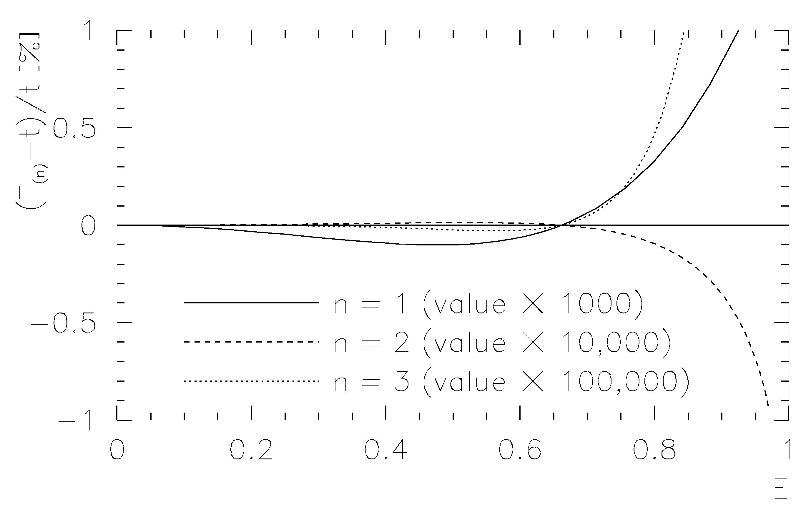
where $D=\Delta E_1\Delta E_2\Delta E_3(\Delta E_1-\Delta E_2)(\Delta E_1-\Delta E_3)(\Delta E_2-\Delta E_3)$. For $0\le E\le 0.70$, the relative deviation was restricted to $5·{10}^{-10}$, while up to $E=0.92$, the maximal relative deviation was $4·{10}^{-8}$. The results for the deviations of $T_{\left(n\right)}$ ($n=1,2,3$) for linear, quadratic, and cubic dynamical approximation are shown in Figure 2.

5. Discussion

In order to test the feasibility and speed, we coded our algorithm in the computer language C under Slackware 15.0 (Linux 5.15.19) on an ordinary HP laptop with an Intel® Core™2 Duo CPU P8600 @ 2.4GHz with 3MB memory used. The dependence of the CPU time for the calculation was estimated by calculating the value ${10}^6$ times in sequence. The speed of the calculation did not depend on the value for E, as the precision was not optimized. This would be required for practical application. Using an arbitrary starting value $E=0.8$, we performed this test, and the results are shown in

Table 1. Runtime experiment for our algorithm under C for $E=0.8$ and different values of n and p (CPU time in seconds). As indicated, the errors are in the last displayed digit, i.e., $\pm 0.01$ s.

	$\mathit{n}=0$	$\mathit{n}=1$	$\mathit{n}=2$	$\mathit{n}=3$	$\mathit{n}=4$	$\mathit{n}=5$
$p=0$	$0.07\left(1\right)$	$0.13\left(1\right)$	$0.17\left(1\right)$	$0.21\left(1\right)$	$0.31\left(1\right)$	$0.56\left(1\right)$
$p=1$	$0.14\left(1\right)$	$0.20\left(1\right)$	$0.24\left(1\right)$	$0.29\left(1\right)$	$0.39\left(1\right)$	$0.63\left(1\right)$
$p=2$	$0.25\left(1\right)$	$0.32\left(1\right)$	$0.35\left(1\right)$	$0.40\left(1\right)$	$0.50\left(1\right)$	$0.75\left(1\right)$

. An analysis of this table showed that a further step in the degree p doubled the runtime while the dynamics for increasing n added a constant value of approximately $0.06$ seconds to the result. Though the increase in the dynamics required the solution of a linear system of equations and the coding of the results, this endeavor was justified, as by using the dynamics, we could increase the precision of the results without sacrificing the computational speed.

The results for the deviations in Figure 1 and Figure 2 were multiplied by increasing the decimal powers in order to ensure the results were comparable. This indicated that the convergence was improved in each of the steps for p and n, at least by the corresponding inverse power, while the static approximations $n=0$ in Figure 1 showed both deviations were close to $E=0$, and for higher values of E, the dynamical approximations in Figure 2 showed no deviation at $E=0$ and moderate deviations for higher values. However, the costs for an improvement step in either p or n was, at most, a 2-fold increase in CPU time. This indicated that the calculations and coding of expressions such as Equation (9) were justified by the increased precision. Given the goals for the precision, the user could decide to which degrees of p and n the algorithm should be developed. In order to prove the precision, in

Table 2. Results for $p=2$ and increasing values of n for values of E approaching $E=1$. The last column shows the CPU time for ${10}^6$ runs according to the algorithm proposed in [12] for the values of N, given in the last column of the table displayed in [12].

$\mathit{E}=$	$\mathit{n}=0$	$\mathit{n}=1$	$\mathit{n}=2$	$\mathit{n}=3$	$\mathit{n}=4$	$\mathit{n}=5$	[12]
$0.7$	$0.732995$	$0.732868$	$0.732869$	$0.732869$	$0.732869$	$0.732869$	$0.17$
$0.8$	$0.906326$	$0.906193$	$0.906194$	$0.906194$	$0.906194$	$0.906194$	$0.19$
$0.9$	$1.163247$	$1.163085$	$1.163087$	$1.163087$	$1.163087$	$1.163087$	$0.35$
$0.99$	$1.821691$	$1.821376$	$1.821387$	$1.821386$	$1.821386$	$1.821386$	$1.95$
$0.999$	$2.326608$	$2.326762$	$2.326752$	$2.326754$	$2.326754$	$2.326754$	$14.62$
$0.9999$	$2.749217$	$2.751197$	$2.751034$	$2.751076$	$2.751056$	$2.751971$	$128.30$

, we showed the convergence of our procedure for $p=2$ with fixed and increasing values of n. The last column shows the CPU times for ${10}^6$ runs of the algorithm proposed in [12] with N given in the last column of the table in [12], as coded in C.

6. Conclusions

In this paper, we developed and described an approximation algorithm for the determination of the error function, which was based on geometric considerations. As demonstrated in this paper, the algorithm can be easily implemented and extended. We showed that each improvement step improved the precision by a factor of ten or more, with an increase in CPU time of, at most, a factor of two or more. In addition, we provided a geometric derivation of Craig’s integral representation of the error function and a converging power series expansion for this formula.

References

1. Von Neumann, J. Various Techniques Used in Connection with Random Digits. In Monte Carlo Methods; Householder, A.S., Forsythe, G.E., Germond, H.H., Eds.; National Bureau of Standards Applied Mathematics Series; Springer: Berlin, Germany, 1951; Volume 12, pp. 36–38. [Google Scholar]
2. Quside Unveils the World’s First Randomness Processing Unit. Available online: https://quside.com/quside-unveils-the-worlds-first-randomness-processing-unit (accessed on 27 February 2023).
3. Craig, J.W. A new, simple and exact result for calculating the probability of error for two-dimensional signal constellations. In Proceedings of the 1991 IEEE Military Communication Conference, McLean, VA, USA, 4–7 November 1991; Volume 2, pp. 571–575. [Google Scholar]
4. Lever, K.V. New derivation of Craig’s formula for the Gaussian probability function. Electron. Lett. 1998, 34, 1821–1822. [Google Scholar] [CrossRef]
5. Tellambura, C.; Annamalai, A. Derivation of Craig’s formula for Gaussian probability function. Electron. Lett. 1999, 35, 1424–1425. [Google Scholar] [CrossRef] [Green Version]
6. Stewart, S.M. Some alternative derivations of Craig’s formula. Math. Gaz. 2017, 101, 268–279. [Google Scholar] [CrossRef]
7. Martila, D.; Groote, S. Evaluation of the Gauss Integral. Stats 2022, 5, 32. [Google Scholar] [CrossRef]
8. Andrews, L.C. Special Functions of Mathematics for Engineers; SPIE Press: Oxford, UK, 1998; p. 110. [Google Scholar]
9. Strecok, A.J. On the Calculation of the Inverse of the Error Function. Math. Comp. 1968, 22, 144–158. [Google Scholar]
10. Blair, J.M.; Edwards, C.A.; Johnson, J.H. Rational Chebyshev Approximations for the Inverse of the Error Function. Math. Comp. 1976, 30, 827–830. [Google Scholar] [CrossRef]
11. Bergsma, W.P. A new correlation coefficient, its orthogonal decomposition and associated tests of independence. arXiv 2006, arXiv:math/0604627. [Google Scholar]
12. Dominici, D. Asymptotic analysis of the derivatives of the inverse error function. arXiv 2007, arXiv:math/0607230. [Google Scholar]
13. Dominici, D.; Knessl, C. Asymptotic analysis of a family of polynomials associated with the inverse error function. arXiv 2008, arXiv:0811.2243. [Google Scholar] [CrossRef]
14. Winitzki, S. A Handy Approximation for the Error Function and Its Inverse. Available online: https://www.academia.edu/9730974/ (accessed on 27 February 2023).
15. Giles, M. Approximating the erfinv function. In GPU Computing Gems Jade Edition; Applications of GPU Computing Series; Morgan Kaufmann: Burlington, MA, USA, 2012; pp. 109–116. [Google Scholar]
16. Soranzo, A.; Epure, E. Simply Explicitly Invertible Approximations to 4 Decimals of Error Function and Normal Cumulative Distribution Function. arXiv 2012, arXiv:1201.1320. [Google Scholar]
Figure 1. Relative deviations for the static approximations.
Stats 06 00026 g001
Figure 2. Relative deviations for the dynamical approximations (the degree was set as p = 1 ).
Stats 06 00026 g002