Article

Quantile Regression Approach for Analyzing Similarity of Gene Expressions under Multiple Biological Conditions

by
Dianliang Deng
1,*,† and
Mashfiqul Huq Chowdhury
2,†
1
Department of Mathematics and Statistics, University of Regina, Regina, SK S4S 0A2, Canada
2
Department of Statistics, Mawlana Bhashani Science and Technology University, Santosh, Tangail 1902, Bangladesh
*
Author to whom correspondence should be addressed.
These authors contributed equally to this work.
Stats 2022, 5(3), 583-605; https://doi.org/10.3390/stats5030036
Submission received: 6 June 2022 / Revised: 27 June 2022 / Accepted: 29 June 2022 / Published: 2 July 2022

Abstract

:
Temporal gene expression data contain ample information to characterize gene function and are now widely used in bio-medical research. A dense temporal gene expression usually shows various patterns in expression levels under different biological conditions. The existing literature investigates the gene trajectory using the mean function. However, temporal gene expression curves usually show a strong degree of heterogeneity under multiple conditions. As a result, rates of change for gene expressions may be different in non-central locations and a mean function model may not capture the non-central location of the gene expression distribution. Further, the mean regression model depends on the normality assumptions of the error terms of the model, which may be impractical when analyzing gene expression data. In this research, a linear quantile mixed model is used to find the trajectory of gene expression data. This method enables the changes in gene expression over time to be studied by estimating a family of quantile functions. A statistical test is proposed to test the similarity between two different gene expressions based on estimated parameters using a quantile model. Then, the performance of the proposed test statistic is examined using extensive simulation studies. Simulation studies demonstrate the good statistical performance of this proposed test statistic and show that this method is robust against normal error assumptions. As an illustration, the proposed method is applied to analyze a dataset of 18 genes in P. aeruginosa, expressed in 24 biological conditions. Furthermore, a minimum Mahalanobis distance is used to find the clustering tree for gene expressions.

1. Introduction

Recently, many researchers have focus on the analysis of gene expression data. The gene expression process records measurements of expression under various biological conditions over a specific time period. At present, micro-array experiments are widely being used to generate rapidly vast amounts of data on gene expression under various biological conditions. The analysis of temporal gene expression is now becoming of great interest to scientists to understand the complex mechanism of gene profiles and characterize gene expressions. Moreover, this analysis also helps bio-medical scientists detect the genes responsible for early cancer (Fang et al. [1]). Genes are generally expressed by transcription into RNA, and then this transcript might be translated into protein. Usually, the gene expression process conveys RNA information as numerical outcomes. For gene expression data, specific biological characteristics (for example, RNA information) are usually measured during a predetermined time interval under different experimental conditions.
Several statistical methods to analyze gene expression data have been considered, including clustering, fold expression changes, ANOVA, etc. Draghici and Kulaeva [2] discussed a noise sampling method based on ANOVA for the selection of differentially regulated genes. They compared their results with the fold change method and discussed the risk of obtaining a false positive when strictly observing fold change. Eisen et al. [3] used a cluster analysis method to compare genes according to similarity. Li et al. [4] introduced a time-lagged correlation coefficient to assess the relationship between genes and used the linear mixed-effect model with splines for gene clustering. Yeung and Ruzzo [5] applied the principal component analysis to analyze gene expression data. They also studied the effectiveness of different clustering algorithms to capture cluster structure. Fang et al. [1] discussed some limitations of the fold expression method, suggesting that genetic information might be lost using this method. One defining feature of gene expression analysis is its time-dependency on the expression levels for a given gene at multiple times. Therefore, it is very important to incorporate the correlation structure within gene expressions. Kerr et al. [6], Storey and Tibshirani [7] studied differentially expressed genes from a single timepoint. Meanwhile, Tusher et al. [8] developed a temporal gene expression model based on one condition. Fang et al. [1] proposed a non-linear regression model to mark the relative change rates of genes. Their study uses changeable variance and covariance structure to model individual gene expression trajectory. Deng et al. [9] investigated the effects of different biological conditions on gene expressions. Under a given condition, Deng et al. [9] used log-normal distribution properties to characterize the variance function of genes and proposed a statistical test approach to test the equality of the variance function for different conditions. Deng et al. [10] studied the threshold points of the gene expressions and constructed test statistics to detect the threshold points.
At present, the available literature only considers using the mean function when analyzing gene expression trajectory. However, when gene expression data are skewed or over-dispersed, the mean function can be affected by outlying observations. Normality is usually assumed as the error term for estimation of the parameters in the model, and this assumption may be improper in practical instances. In addition, the temporal gene expression curve generally shows a strong degree of heterogeneity between multiple biological conditions. As a result, the rates of change for gene expressions may be different in non-central locations, and the mean model can only characterize the central location of the gene expression distribution. Thus, mean function may not properly capture the gene expression trajectory. However, by fitting the gene expression curves at different quantile vaules, the quantile regression approach can be used to completely examine the gene expression rate. Many researchers have explored statistical methods for the analysis of the quantile regression model. Huang and Lee [11] predicted the quantiles of daily Standard&Poor’s 500 (S&P 500) returns by incorporating the high-frequency information through combining forecasts into one model. Most recently, Gallardo et al. [12] proposed a parametric quantile regression model for asymmetric response variables. Jung et al. [13] applied the multiple quantile regression method to the estimation of the spatial distribution of soil moisture. Chen et al. [14] studied estimation and inference for linear quantile regression models with generated regressors using a practical, two-step estimation procedure. Nevertheless, to our knowledge, there is no literature examining the gene expression data using the quantile regression model.
The purpose of this research is to apply the quantile regression (QR) model to the analysis of gene expression data and propose a test statistic for the examination of the similarity between gene expressions by comparing the quantile regression coefficients. The remainder of this article is organized as follows. In Section 2, the quantile regression model is proposed for gene expression data and the statistical inference is given for this model. The simulation study is performed in Section 3. An application for gene expression data is presented in Section 4, with the discussion in Section 5.

2. Quantile Model for Gene Expression Data

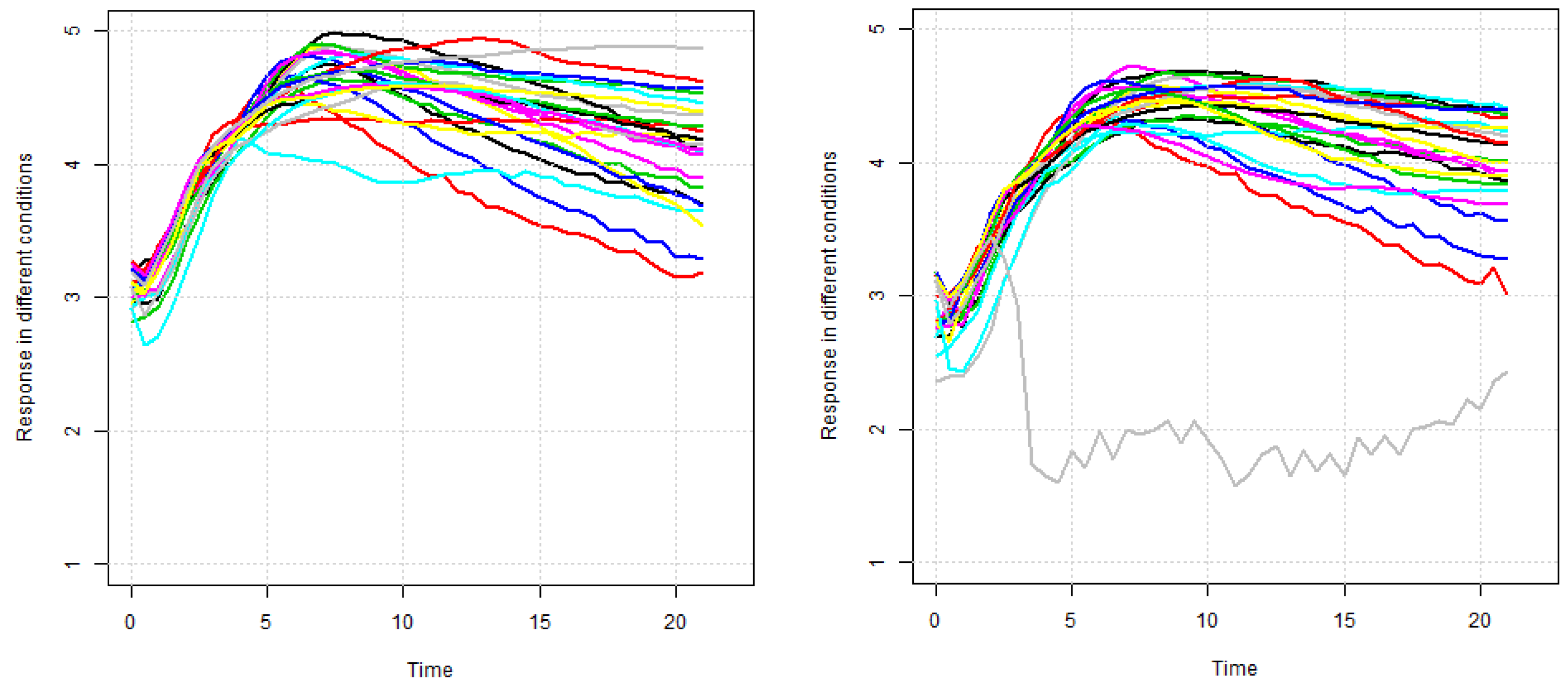
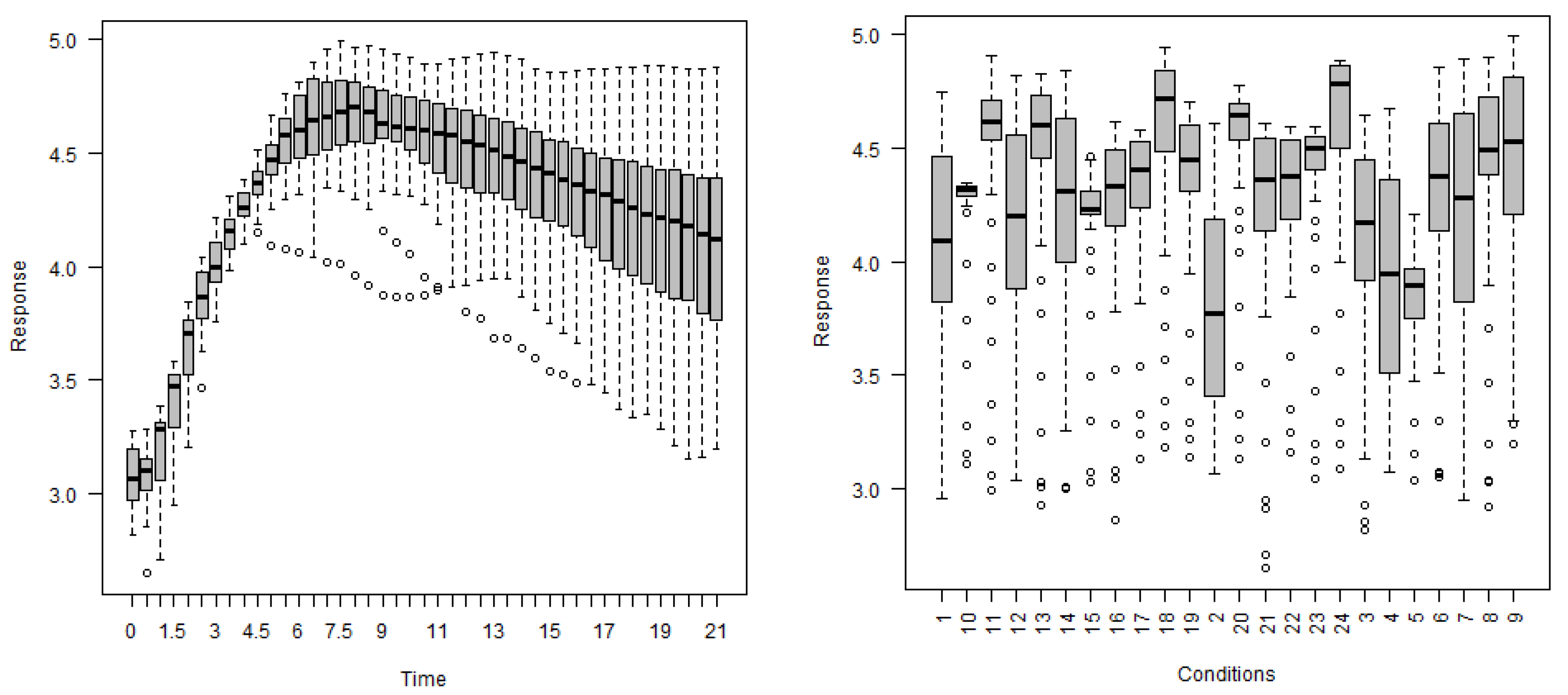
In this section, this research methodology is introduced to analyze the gene expression data. In most cases, for gene expression data, specific characteristics were measured at discrete timepoints and measurements were taken under different biological conditions. As gene expression characteristics were measured over a series of timepoints and repeated under different circumstances, the longitudinal data analysis method can be applied to analyze discrete gene expression data. On the other hand, gene expression measurements show a variety of patterns under different biological conditions over specific times. Therefore, the linear quantile mixed model may be appropriate for the analysis of gene expression data. Let Y i ( t ) be the observed measurement of specific gene expression under the i t h condition at time t. To determine the gene trajectory at different quantiles τ ( 0 < τ < 1 ) , the following quantile model for Y i ( t ) can be considered.
Y i ( t ) = Q ( τ ) ( t ) + ϵ i ( τ ) ( t ) ; i = 1 , , N ,
where, Q ( τ ) ( t ) is the quantile curve at time t, ϵ i ( τ ) ( t ) is the random noise with zero τ th quantile and N denotes the number of conditions. Note that we are unable to observe Y i ( t ) for all timepoints, only at the very specific occasions t i j at which measurements with errors were taken. Therefore, the observed longitudinal data for a specific gene under i t h biological condition consist of the measurements y i = { y i ( t i j ) ; j = 1 , k i } , where k i denotes the number of observed timepoints. Note that, for gene expression data, there is no available covariate. However, there are many methods in the literature that can be used to estimate the quantile function Q ( τ ) ( t ) , including kernel, local polynomial, smoothing splines, regression splines and wavelet-based methods, among others. One simple and straightforward basis is the polynomial basis { 1 , t , , t p 1 } , in which the true quantile function of gene trajectory expression is modeled as polynomials of degree p 1 . In this article, the method proposed in Donoho and Johnstone [15] and further developed in Zhang [16] is adopted. In this spline method, Q ( τ ) ( t ) is approximated using the linear combination of a set of truncated power basis functions. Given a sequence of K interior knots 0 < κ 1 < κ 2 < < κ K < T where T is the end time of observations, the regression spline basis functions of order p are 1 , t , t 2 , , t p , ( t κ 1 ) + p , , ( t κ K ) + p . Denoting the vector of r ( = K + 1 + p ) basis functions by
B ( t ) = ( 1 , t , t 2 , , t p , ( t κ 1 ) + p , , ( t κ K ) + p ) ,
the regression spline smoothing is used to model Q ( τ ) ( t ) using the linear combination of the basis functions B ( t ) , and the linear quantile mixed model can be written as
Y i ( t ) = [ B ( t ) ] β ( τ ) + [ Z ( t ) ] U ( τ ) + ϵ i ( τ ) ( t ) ;
where the basis function for the fixed effects parameter is denoted as B ( t ) = ( 1 , t , t 2 , , t q , ( t κ 1 ) + q , , ( t κ K ) + q ) and Z ( t ) is considered as basis function for random effects parameter, which could be the q-dimensional sub-vector of B ( t ) ( q r ) . In particular, basis functions for the random intercept model and random slope model can be written as follows:
  • Random intercept model, Z ( t ) = ( 1 ) ;
  • Random slope model Z ( t ) = ( 1 , t ) .
For model formulation, gene expression data are considered longitudinal data in the form { Y i ( t i j ) , B ( t i j ) , Z ( t i j ) } , for n biological conditions and k i time occasions, i.e., i = 1 , 2 , , n and j = 1 , 2 , , k i . Now, define
Y i = Y i ( t i 1 ) Y i ( t i 2 ) Y i ( t i k i ) , B i = B ( t i 1 ) B ( t i 2 ) B ( t i k i ) , Z i = Z ( t i 1 ) Z ( t i 2 ) Z ( t i k i ) , ϵ i ( τ ) = ϵ i 1 ( τ ) ϵ i 2 ( τ ) ϵ i k i ( τ )
and β ( τ ) = ( β 1 ( τ ) , , β r ) , U i ( τ ) = ( U i 1 ( τ ) , , U i q ( τ ) ) . Then, we have the matrix form of the model (2) as follows:
Y i = B i β ( τ ) + Z i U i ( τ ) + ϵ i ( τ )
Now, for a longitudinal setup, assuming that Y i conditioned on random effects, U i are independently distributed and this conditional distribution follows the asymmetric Laplace (AL) distribution with location parameter μ i ( τ ) = B i β ( τ ) + Z i U i ( τ ) and scale parameter σ ( τ ) , respectively. Therefore, it can be written as
Y i | U i ( τ ) A L ( B i β ( τ ) + Z i U i ( τ ) , σ ( τ ) , τ ) ,
where β ( τ ) denotes the r × 1 vector of fixed-effect parameters and τ is considered the quantile level. Assume that random effect vectors U i ( τ ) are zero τ -quantile vectors and independent of the error term ϵ i ( τ ) of the model ( U i ( τ ) ϵ i ( τ ) ). Moreover, assume that random effect vectors U i ( τ ) are distributed with the density function f ( u i ( τ ) | Ψ ( τ ) ) , where Ψ ( τ ) is regarded as the variance–covariance matrix (symmetric positive definite). All parameters depend on the skewness parameter, τ ( 0 < τ < 1 ) . Now, the τ th linear quantile mixed model can be written as
Y = μ ( τ ) + ϵ ( τ ) ,
where Y = ( Y 1 , Y 2 , , Y n ) , μ ( τ ) = ( μ 1 ( τ ) , μ 2 ( τ ) , , μ n ( τ ) ) and i.i.d components of error ϵ ( τ ) = ( ϵ 1 ( τ ) , ϵ 2 ( τ ) , , ϵ n ( τ ) ) follow an asymmetric Laplace distribution. Symbolically, ϵ i j ( τ ) A L ( 0 , σ , τ ) , i = 1 , 2 , , n ; j = 1 , 2 , , k i . Now, in terms of matrix notation, τ th linear quantile of response ( Y ) , denoted as μ ( τ ) , can also be expressed as
μ ( τ ) = B β ( τ ) + Z U ( τ ) ,
where, U ( τ ) = ( U 1 , U 2 , , U n ) , Z = i = 1 n Z i and B = ( B 1 , B 2 , , B n ) .

2.1. Estimation of Parameters

Based on the above discussion, the joint density of ( Y , U ( τ ) ) can be written in terms of the τ th quantile as follows:
f ( y , u ( τ ) | β ( τ ) , Ψ | ( τ ) , σ ( τ ) ) = f ( y | β ( τ ) , u ( τ ) , σ ( τ ) ) f ( u ( τ ) | Ψ ( τ ) ) = i = 1 n f ( y i | β ( τ ) , u i ( τ ) , σ ( τ ) ) f ( u i ( τ ) | Ψ ( τ ) )
For the random intercept model ( q = 1 ) , the design matrix for random effects can be written as Z i = ( 1 , 1 , , 1 ) ; i = 1 , 2 , , n . Let, R q denote q dimensional Euclidean space. Now, the marginal likelihood can be derived from Equation (5) and written as
L i ( β ( τ ) , σ ( τ ) , Ψ ( τ ) | y ) = R q f ( y i | β ( τ ) , u i ( τ ) , σ ( τ ) ) f ( u i ( τ ) | Ψ ( τ ) ) d u i
Moreover, the marginal log-likelihood function can also be written as
l i ( β ( τ ) , σ ( τ ) , Ψ ( τ ) | y ) = log L i ( β ( τ ) , σ ( τ ) , Ψ ( τ ) | y ) .
Since the distribution of Y ( t i j ) is assumed to follow an asymmetric Laplace distribution, τ th quantile of Y ( t i j ) can be estimated using the asymmetric Laplace distribution with location parameter μ i j ( τ ) = μ ( τ ) ( t i j ) = [ B ( t i j ) ] β ( τ ) + [ Z ( t i j ) ] U i ( τ ) , common scale σ ( τ ) parameter and known skew parameter ( τ ) . To estimate parameters from joint density f ( y , u ( τ ) ) , expressed in Equation (5), it is important to compute the following integral, which is also known as the marginal density of Y i .
f ( y i | β ( τ ) , σ ( τ ) , Ψ ( τ ) ) = σ k i ( τ ) R q exp 1 σ ρ τ ( y i μ i ( τ ) ) f ( u i | Ψ ( τ ) ) d u i ,
where, σ k i ( τ ) = τ ( 1 τ ) σ k i and
ρ τ ( y i μ i ( τ ) ) = j = 1 k i ρ τ ( y i j μ i j ( τ ) ) = j = 1 k i ρ τ ( y ( t i j ) [ B ( t i j ) ] β ( τ ) [ Z ( t i j ) ] U i ( τ ) )
Now, the log-likelihood function for n conditions can be expressed as
l ( β ( τ ) , σ ( τ ) , Ψ ( τ ) | y ) = i = 1 n log ( σ k i ( τ ) ) + log R q exp 1 σ ρ τ ( y i μ i ( τ ) ) f ( u i | Ψ ( τ ) ) d u i
This numerical likelihood can be solved by applying Gaussian quadrature (Gauss–Hermite quadrature or Gauss–Laguerre quadrature) proposed by Geraci and Bottai [17]. Now, assuming normal random effects ( U i N ( 0 , Ψ ( τ ) ) ) to Equation (9), the Gauss–Hermite quadrature can be applied to approximate the likelihood function with nodes ν m 1 , , m q = ( ν m 1 , , ν m q ) and weights w m l , l = 1 , 2 , , q , respectively. Integer M determines the number of points over the real line for each of the q one-dimensional integrals. The covariance matrix of the random effects is reparameterized by parameters α ( τ ) , i.e., Ψ ( α ( τ ) ) , and parameters, characterized by β ( τ ) and α ( τ ) , are denoted by θ ( τ ) = ( β ( τ ) , α ( τ ) ) T . Finally, Equation () leads to the following approximate likelihood.
l a p p ( θ ( τ ) , σ ( τ ) | y ) = i = 1 n log m 1 = 1 M m q = 1 M f ( y i | β ( τ ) , σ ( τ ) , [ Ψ ( α ( τ ) ) ] 1 2 ν m 1 , , m q ) l = 1 q w m l .
Geraci and Bottai [17] develop the gradient search (gs) and the derivative free (df) optimization algorithm to maximize likelihood function in Equation (10). This optimization starts with a parameter value and then searches the positive semi-line for a new parameter value where likelihood is larger. This algorithm works until the likelihood change is sufficiently small or less than the pre-specified tolerance ( δ ) level. This algorithm begins estimating by initializing β ( τ ) = β 0 ( τ ) ; α ( τ ) = α 0 ( τ ) ; σ ( τ ) = σ 0 ( τ ) . The derivative-free optimization algorithm is similar to the gradient search method. This method alternates a loop for θ ( τ ) and then updates σ ( τ ) .
Now, from the approximate likelihood in Equation (10), the fixed effects parameter β ( τ ) , the random effects parameter α ( τ ) and the error term parameter σ ( τ ) can be estimated by using the algorithm given in Geraci and Bottai [17]. Further, the estimate of quantile function Q ( τ ) ( t ) can be written as follows
Q ^ ( τ ) ( t ) = [ B ( t ) ] β ^ ( τ ) + [ Z ( t ) ] U ^ ( τ )
where β ^ ( τ ) is the estimate of β ( τ ) and U ^ ( τ ) is the estimated best linear predictor of U ( τ ) , which can be expressed as (Geraci and Botai [17])
U ^ ( τ ) = Ψ ^ ( τ ) Z Σ ^ 1 { Y B β ^ ( τ ) E ^ ( ϵ ( τ ) ) }
where Ψ ^ ( τ ) = Ψ ( α ^ ( τ ) ) , Z = ( Z 1 , , Z n ) , Σ ^ = cov ^ ( Y ) = Z Ψ ^ ( τ ) Z + cov ^ ( ϵ ( τ ) ) = Z Ψ ^ ( τ ) Z + diag ( var ^ ( ϵ i j ( τ ) ) ) with var ^ ( ϵ i j ( τ ) ) = σ ^ ( τ ) ( τ 2 + ( 1 τ ) 2 ) τ 2 ( 1 τ ) 2 , j = 1 , , k i ; i = 1 , , n and E ^ ( ϵ ( τ ) ) = ( E ^ ( ϵ 11 ( τ ) ) , , E ^ ( ϵ 1 k 1 ( τ ) ) ; ; E ^ ( ϵ n 1 ( τ ) ) , , E ^ ( ϵ n k n ( τ ) ) ) with E ^ ( ϵ i j ( τ ) ) = σ ^ ( τ ) ( 1 2 τ ) τ ( 1 τ ) for j = 1 , , k i ; i = 1 , , n . Furthermore, the asymptotic covariance matrix for U ^ ( τ ) can be derived as
cov ( U ^ ( τ ) ) = Ψ ^ ( τ ) Z Σ ^ 1 Z Ψ ^ ( τ ) Z Σ ^ 1 Z Ψ ^ ( τ )
Asymptotically, Q ^ ( τ ) ( t ) N ( Q ( τ ) ( t ) , V ^ Q ( τ ) ( t ) ) with
V ^ Q ( τ ) ( t ) = var ^ ( Q ^ ( τ ) ( t ) ) = ( B ( t ) , Z ( t ) ) cov ^ ( β ^ ( τ ) , U ^ ( τ ) ) ( B ( t ) , Z ( t ) )
From the asymptotic normality of
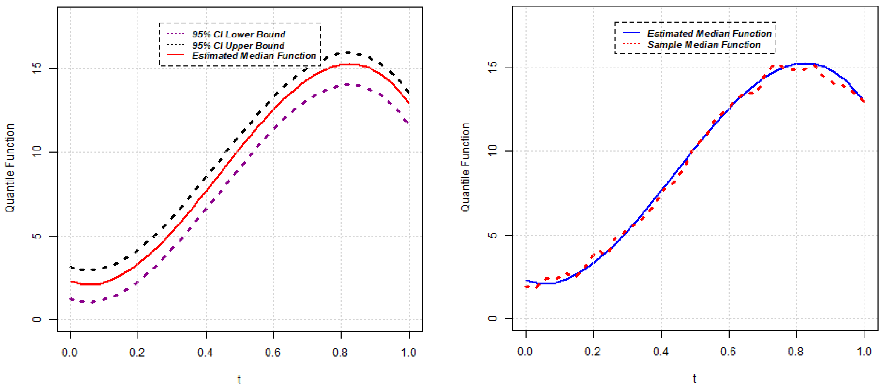
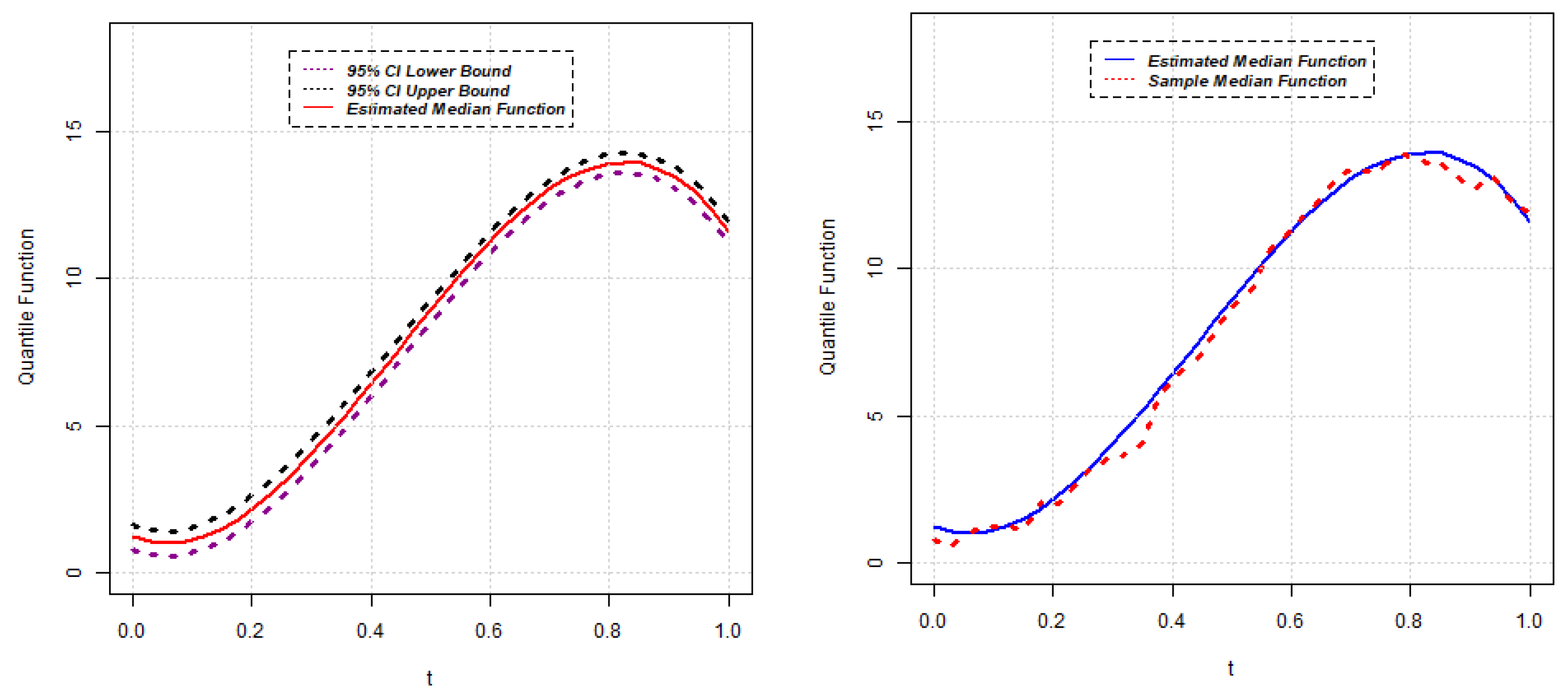
 Q ^ ( τ ) ( t ) , the approximate ( 1 α ) 100 % confidence interval for the quantile function Q ( τ ) ( t ) can be constructed as follows:
Q ^ ( τ ) ( t ) ± z α 2 V ^ Q ( τ ) ( t )
where z α 2 is the upper 100 ( 1 α 2 ) % percentile of standard normal distribution. Although the asymptotic covariance matrix for U ^ ( τ ) has a closed form (12), there is no expression for the covariance matrix of estimator β ^ ( τ ) , and thus we are unable to find the expression for the estimate of covariance cov ^ ( β ^ ( τ ) , U ^ ( τ ) ) . However, bootstrap is a very powerful method and can be used in the estimation of covariance matrix for estimators ( β ^ ( τ ) , U ^ ( τ ) ) . Here, we use a block bootstrap approach to find the estimate for cov ^ ( β ^ ( τ ) , U ^ ( τ ) ) .
The procedures are as follows.
1.
Obtain R bootstrap samples from the original data { Y i ( t i j ) , B ( t i j ) , Z ( t i j ) ; j = 1 , 2 , , k i ; i = 1 , 2 , , n }
2.
Find the estimated values for the parameters β ( τ ) , α ( τ ) and σ ( τ ) and then calculate the values of U ^ ( τ ) by using formula (11) from each bootstrap sample and denote the obtained values as β ^ 1 ( τ ) , , β ^ R ( τ ) ; α ^ 1 ( τ ) , , α ^ R ( τ ) ; σ ^ 1 ( τ ) , , σ ^ R ( τ ) and U ^ 1 ( τ ) , , U ^ R ( τ ) .
3.
Set ϕ ^ r ( τ ) = ( β ^ r ( τ ) , U ^ r ( τ ) ) , ϑ ^ r ( τ ) = ( β ^ r ( τ ) , α ^ r ( τ ) , σ ^ r ( τ ) ) , r = 1 , 2 , R and calculate the sample means of R bootstrap estimates for fixed effects parameters and random effects predictors ϕ ( τ ) = ( β ( τ ) , U ( τ ) ) and ϑ r ( τ ) = ( β r ( τ ) , α r ( τ ) , σ r ( τ ) )
ϕ ¯ ( τ ) = 1 R r = 1 R ϕ ^ r ( τ ) , ϑ ¯ ( τ ) = 1 R r = 1 R ϑ ^ r ( τ )
4.
Now, the bootstrap estimator for covariance matrix of estimators ( β ^ ( τ ) , U ^ ( τ ) ) can be written as
V ^ ϕ ( τ ) = cov ^ ( β ^ ( τ ) , U ^ ( τ ) ) = 1 R 1 r = 1 R ( ϕ ^ r ( τ ) ϕ ¯ ( τ ) ) ( ϕ ^ r ( τ ) ϕ ¯ ( τ ) ) ,
V ^ ϑ ( τ ) = cov ^ ( β r ( τ ) , α r ( τ ) , σ r ( τ ) ) = 1 R 1 r = 1 R ( ϑ ^ r ( τ ) ϑ ¯ ( τ ) ) ( ϑ ^ r ( τ ) ϑ ¯ ( τ ) )
Furthermore, the estimates of model parameters and covariance matrix of estimators are computed by using the ‘lqmm’ package developed by Geraci and Bottai [17] in the R programming environment. Generally, this ‘lqmm’ package is used to estimate conditional quantile functions with random effects in linear quantile mixed models.

2.2. Test of the Similarity of Quantile Functions for Two Gene Expressions

The other purpose of this research is to identify gene similarity based on quantile functions. Using the results obtained in 
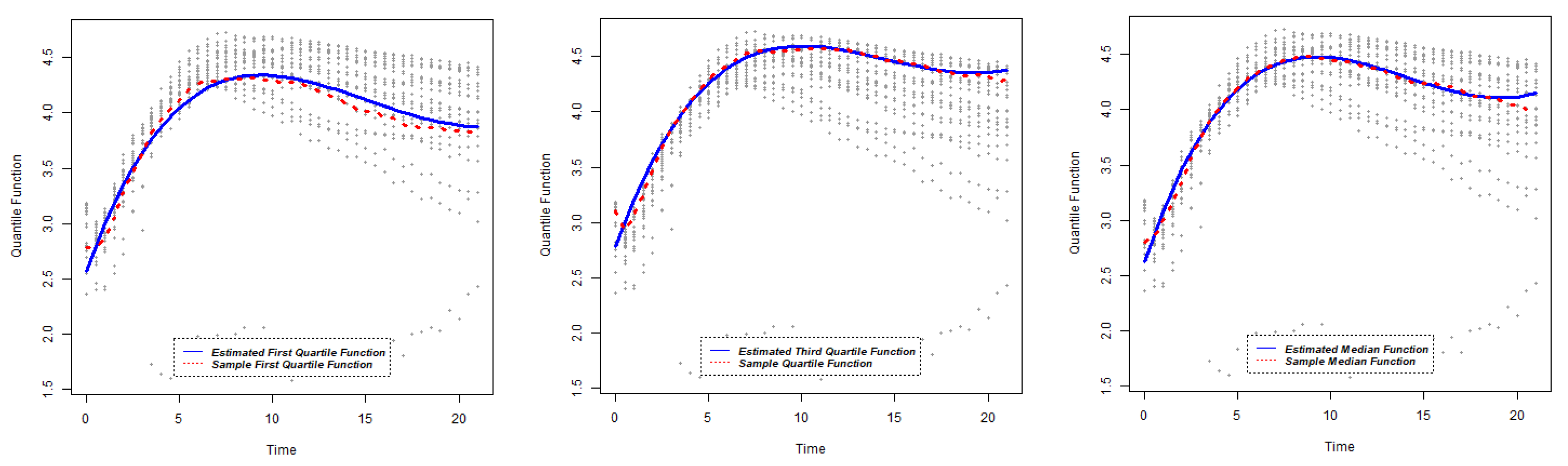
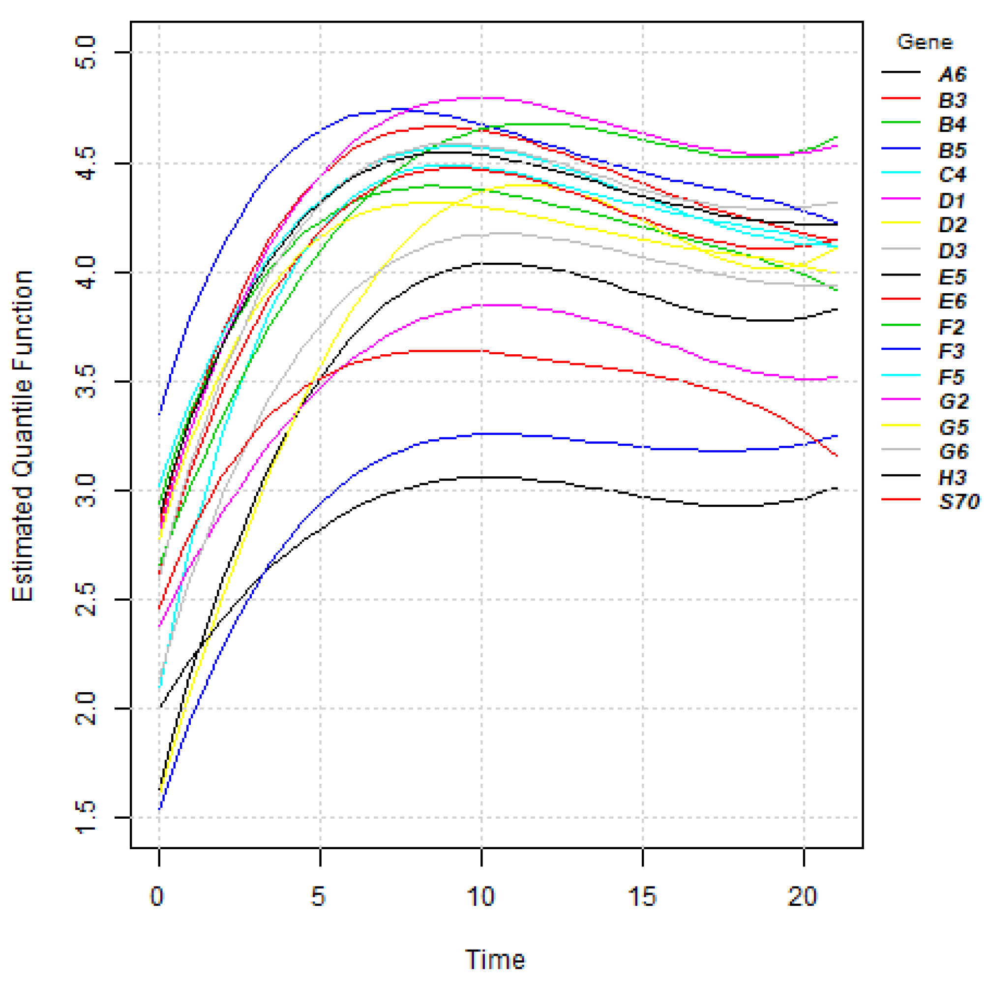
Section 2.1, the estimates of quantile functions for gene expressions can be obtained. The estimated quantile functions for g genes can be expressed as
Q ^ h ( τ ) ( t ) = [ B ( t ) ] β ^ h ( τ ) + [ Z ( t ) ] U ^ h ( τ ) ; h = 1 , 2 , , g .
Two genes, h and s, are said to be similar if their quantile curve expressions are equal, i.e.,
Q ^ h ( τ ) ( t ) = Q ^ s ( τ ) ( t ) ; t [ 0 , T ] , T > 0 .
Therefore, the proposed hypothesis is
H 0 : Q h ( τ ) ( t ) = Q s ( τ ) ( t ) vs H 1 : Q h ( τ ) ( t ) Q s ( τ ) ( t ) .
Now, suppose that all quantile functions share the same truncated power basis functions B ( t ) and Z ( t ) . Then, the τ –quantile curves of gene expressions depend on the fixed effects parameter β ( τ ) and the random effects components U ( τ ) , and testing the similarity of two gene expression is equivalent to testing the equality of the corresponding fixed effects parameters and random effects components. Further, the predictors of random effects components depend on the estimates of parameters β ( τ ) T , α ( τ ) , σ ( τ ) . Thus, instead of testing the hypothesis (17), one can test the following hypothesis related to the fixed effects parameters and the random effects components.
H 0 : ( β h ( τ ) , α h ( τ ) , σ h ( τ ) ) = ( β s ( τ ) , α s ( τ ) , σ s ( τ ) ) vs H 1 : ( β h ( τ ) , α h ( τ ) , σ h ( τ ) ) ( β s ( τ ) , α s ( τ ) , σ s ( τ ) ) .
Based on parameter estimates and its covariance matrix, the following asymptotic statistic for testing the the hypothesis H 0 : ( β h ( τ ) , α h ( τ ) , σ h ( τ ) ) = ( β s ( τ ) , α s ( τ ) , σ s ( τ ) ) ; ( h s ) , is given by
χ h s 2 ( τ ) = β ^ h ( τ ) β ^ s ( τ ) α ^ h ( τ ) α ^ s ( τ ) σ ^ h ( τ ) σ ^ s ( τ ) Ξ β ^ h ( τ ) β ^ s ( τ ) α ^ h ( τ ) α ^ s ( τ ) σ ^ h ( τ ) σ ^ s ( τ ) ,
where, Ξ = ( V ^ β h ( τ ) , α h ( τ ) , σ h ( τ ) h + V ^ β s ( τ ) , α s ( τ ) , σ s ( τ ) s ) 1 and V ^ β h ( τ ) , α h ( τ ) , σ h ( τ ) h and V ^ β s ( τ ) T , α s ( τ ) , σ s ( τ ) s are the estimated variance–covariance matrices of the estimators ( β h ( τ ) , α h ( τ ) , σ h ( τ ) ) and ( β s ( τ ) , α s ( τ ) , σ s ( τ ) ) , respectively, which can be computed from (16). When H 0 holds, χ h s 2 ( τ ) in Equation (19) has asymptotic chi-squared distribution with ( r + q + 1 ) degrees of freedom, where r is known as the dimension number of β ( τ ) for fixed effects parameters and q is the dimension number of α ( τ ) for random effects components.
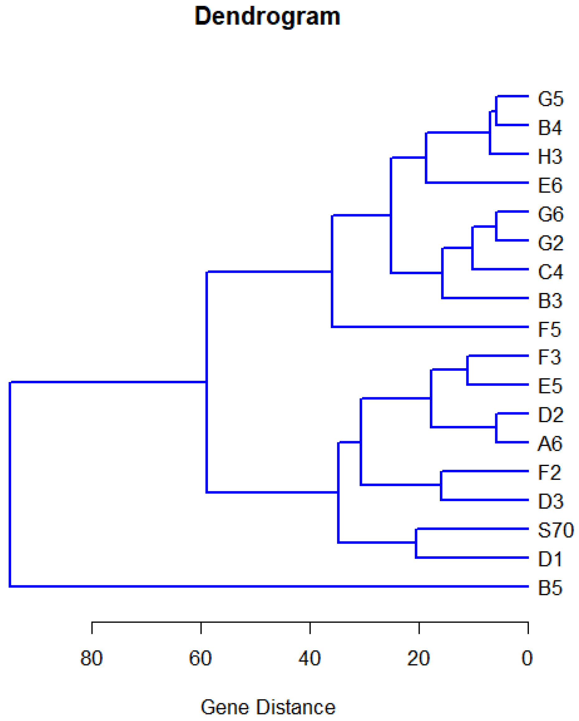
Furthermore, since the quantile function of gene expression is determined by r-dimensional fixed parameters, q-dimensional random effects components, and scale parameter σ ( τ ) , the pattern of gene expression h can be induced to be a random point in the ( r + q + 1 ) dimensional Euclidean space, which has the asymptotic multivariate normal distribution with mean ( β h ( τ ) , α h ( τ ) , σ h ( τ ) ) and covariance matrix V ^ β h ( τ ) , α h ( τ ) , σ h ( τ ) h for h = 1 , , g . From this point of view, the statistic χ h s 2 ( τ ) in (19) is also the Mahalanobis distance between random vectors ( β ^ h ( τ ) , α h ( τ ) , σ h ( τ ) ) and ( β ^ s ( τ ) , α s ( τ ) , σ s ( τ ) ) . In terms of the minimum Mahalanobis distance, we can obtain the clustering tree for g gene expressions.

3. Simulation

In this section, we examine the performance of the estimation and chi-square test (19) based on the proposed quantile model for analyzing temporal gene expression data. Extensive simulation studies are carried out to evaluate the accuracy of the estimated quantile curves and the power of the proposed chi-square test (19). The random intercept QR model and random slope QR model are chosen with five different error terms, in which the error terms are chosen from symmetric distribution (normal), symmetric and heavy tailed distribution (Laplace and Student t) and skewed distribution (skew normal and skew t). Hence, there are ten different scenarios to examine through the simulation study. The steps are given below.
  • Thirty-five equally spaced timepoints between [0, 1] are considered for 50 samples. The data were generated using the following mixed model. The true model is assumed as follows:
    Y i ( t ) = f 0 ( t ) + U i ( t ) + ϵ i ( t ) ; t [ 0 , 1 ] ,
    where, f 0 ( t ) = exp 5 t 1 + t 3 , i = 1 , , 50 .
  • Random effects components are assumed to follow a normal distribution with a mean of zero and standard deviation of two, i.e., ( U i N ( 0 , 4 ) ) .
  • The following i.i.d errors are considered for true models Equation (20).
    1.
       Model 1: ϵ i ( t ) Laplace(0,1)
    2.
       Model 2: ϵ i ( t ) Normal(0,1)
    3.
       Model 3: ϵ i ( t ) Skew Normal(0,1,1)
    4.
       Model 4: ϵ i ( t ) Skew t(0,1,1,4)
    5.
       Model 5: ϵ i ( t ) t(3)

3.1. Model and Parameter Estimation

For model generalization, the following quantile mixed model is considered:
Y i ( t ) = B ( t ) β ( τ ) + Z ( t ) U i + ϵ i ( τ ) ,
where, B ( t ) and Z ( t ) are the basis functions for fixed and random effects components, respectively. The parameter estimation procedure is illustrated below.
  • Generate data for n = 50 samples using Equation (20).
  • Basis functions for Model (21) are considered as:
    1.
      Random intercept model: B ( t ) = ( 1 , t , t 2 , t 3 ) , Z ( t ) = ( 1 ) .
    2.
      Random slope model: B ( t ) = ( 1 , t , t 2 , t 3 ) , Z ( t ) = ( 1 , t ) .
  • Forthe random slope model, we consider normal random effects with a diagonal variance–covariance matrix. A Gauss–Hermite quadrature with seven noves is considered to approximate the marginal log-likelihood of Equation (10).
  • All parameters are estimated at median ( τ = 0.50 ).
  • A total of 500 bootstrap replications are considered for the estimation of the covariance matrix of the estimators ( β ^ ( τ ) , U ^ ( τ ) ) .
Note that, for simplicity, the interior knots are not added in the basis function B ( t ) in this simulation study. The simulations were also conducted in the scenario for the basis function B ( t ) with the interior knots and the results are similar to those without the interior knots. Furthermore, the simulations for the other values of quantile τ are omitted.

3.2. Simulation Results for Parameter Estimation

3.2.1. Parameter Estimates of Random Intercept QR Model

Parameter estimates for the 50th quantile ( τ = 0.50 ) of the random intercept QR model are reported below for five different scenarios. The estimated median function, along with the confidence interval of each random intercept QR model, is presented in Figure 1, Figure 2, Figure 3, Figure 4 and Figure 5. Again, the estimated 50 th ( τ = 0.50 ) quantile function is also compared with sample median function in each figure.
  • Estimates of parameters in Model 1: β ^ ( τ ) = [ 1.19 , 5.06 , 68.86 , 53.29 ] , α ^ ( τ ) = 1.23 , σ ^ ( τ ) = 0.56 , Ψ ^ ( τ ) = 1.52 .
  • Estimates of parameters in Model 2: β ^ ( τ ) = [ 1.68 , 7.42 , 74.74 , 56.87 ] , α ^ ( τ ) = 1.01 , σ ^ ( τ ) = 0.43 , Ψ ^ ( τ ) = 1.02 .
  • Estimates of parameters in Model 3: β ^ ( τ ) = [ 2.03 , 7.46 , 74.81 , 57.17 ] , α ^ ( τ ) = 1.14 , σ ^ ( τ ) = 0.36 , Ψ ^ ( τ ) = 1.29 .
  • Estimates of parameters in Model 4: β ^ ( τ ) = [ 1.88 , 7.85 , 76.28 , 57.92 ] , α ^ ( τ ) = 1.41 , σ ^ ( τ ) = 0.49 , Ψ ^ ( τ ) = 1.98 .
  • Estimates of parameters in Model 5: β ^ ( τ ) = [ 1.29 , 8.70 , 76.78 , 57.78 ] , α ^ ( τ ) = 1.42 , σ ^ ( τ ) = 0.57 , Ψ ^ ( τ ) = 2.01 .

3.2.2. Parameter Estimates of Random Slope QR Model

Now, the estimates of parameters for the 50 th quantile ( τ = 0.50 ) of the random slope QR model are reported below for five different scenarios and estimated median functions; sample median functions, along with confidence intervals, are shown in Figure 6, Figure 7, Figure 8, Figure 9 and Figure 10.
  • Estimates of parameters in Model 1: β ^ ( τ ) = [ 1.27 , 5.08 , 68.86 , 53.31 ] , α ^ ( τ ) = [ 1.35 , 0.67 ] , σ ^ ( τ ) = 0.54 , Ψ ^ intercept ( τ ) = 1.83 , Ψ ^ time ( τ ) = 0.45 .
  • Estimates of parameters in Model 2: β ^ ( τ ) = [ 0.98 , 6.43 , 72.80 , 55.64 ] , α ^ ( τ ) = [ 1.29 , 0.68 ] , σ ^ ( τ ) = 0.41 , Ψ ^ intercept ( τ ) = 1.68 , Ψ ^ time ( τ ) = 0.46 .
  • Estimates of parameters in Model 3: β ^ ( τ ) = [ 1.92 , 7.43 , 74.85 , 57.15 ] , α ^ ( τ ) = [ 1.79 , 0.73 ] , σ ^ ( τ ) = 0.35 , Ψ ^ intercept ( τ ) = 3.20 , Ψ ^ time ( τ ) = 0.53 .
  • Estimates of parameters in Model 4: β ^ ( τ ) = [ 2.30 , 7.83 , 76.31 , 57.87 ] , α ^ ( τ ) = [ 1.67 , 1.06 ] , σ ^ ( τ ) = 0.46 , Ψ ^ intercept ( τ ) = 2.79 , Ψ ^ time ( τ ) = 1.13 .
  • Estimates of parameters in Model 5: β ^ ( τ ) = [ 1.25 , 8.53 , 76.79 , 57.92 ] , α ^ ( τ ) = [ 1.47 , 0.53 ] , σ ^ ( τ ) = 0.57 , Ψ ^ intercept ( τ ) = 2.16 , Ψ ^ time 2 = 0.29 .

3.3. Power Analysis of Proposed Test Statistic

In this section, the power of the chi-square test presented in Equation (19) is evaluated by considering the alternative model. A constant number, m is added to this alternative model.
The alternative model considered in simulation is as follows:
[ Y i ( t ) ] new = exp ( 5 t 1 + t 3 ) + U i ( t ) + ϵ i ( t ) + m
where, m { 0 , 0.50 , 1.00 , 1.50 , 2.00 , 2.50 , 3.00 } . The L 2 distance between true model and alternative model is m. Here, we assume that random effects ( U i ) and error ( ϵ i ) follow the same distribution. The power analysis is carried out for both the random slope QR model and random intercept QR model. All simulation results are performed for a sample size of n = 30 , 50 and 75 at a level of significance of α = 0.05 and quantile value of τ = 0.25 , 0.50, 0.75 with 1000 replications. Table 1, Table 2 and Table 3 report empirical powers for five random intercept QR models and five random slope models with the quantiles τ = 0.25 , 0.5 and 0.75 . Power analysis results demonstrate that the statistical performance of the proposed chi-square test statistic is good for both random intercept models and random slope models at a 5% level of significance. This indicates that this test statistic can be applied to determine the similarity of two gene expressions.

4. Application: Gene Expression Data

In this section, the linear quantile mixed model given in Section 2 is applied to analyze a real dataset of 18 gene expressions in P. aeruginosa expressed in 24 conditions. Some descriptive measures are discussed at the beginning of this section. Towards the end of this section, the similarities between genes are investigated using the proposed test statistic (Equation (19)) based on quantile functions.

4.1. Data

A description of 18 genes is reported in Table 4. The data observed for these genes are first analyzed by Fang et al. [1] and then by Deng et al. [10] Initially, polymerase chain reaction (PCR) was performed to amplify regions of P. aeruginosa virulence factors. The primers were synthesized using PAO1 genome data according to Duan [18]. PAO1 chromosomal DNA was used as a PCR template and amplified promoter regions were cloned into XhoI-BamHI restriction sites of the plasmid PMS402. Then plasmids were inserted into PAO1 using electroporation. More details regarding DNA manipulation, PCR and transformation procedures can be found in Duan [18]. The promoter activity was measured as counts per second (CPS) of light production using a Victor2 Multilabel counter. TSBDC minimal medium containing EDTA (400 μ g/mL) and (50 μ g/mL) F e c l 3 were used to assay gene expression. The reporter strains were grown overnight and the resulting culture was diluted into 1:200 proportion in a 96-well microtiter plate. Then, the promoter activity of the virulence factors was measured under 24 biological conditions every 30 min for 21 h. These genes were considered as quorum-sensing or quorum-sensing-regulated genes, which play an important role in bio-films formation. Thus, this dataset consists of 18 genes in P. aeruginosa (Table 4) and each gene was observed at 43 consecutive timepoints under 24 conditions. Therefore, the data for each gene consist of 1032 observations and, in total, 18,576 observations are measured for 18 genes.

4.2. Exploratory Analysis

In this section, a summary is provided of the selected gene expression data. Gene expressions, g ( t ) are obtained on a log scale under 24 conditions. Figure 11 exhibits gene expression curves of genes PA2975(rluc) and PA0573, respectively. From this figure, it is evident that the expressions for genes PA2975(rluc) and PA0573 are very different under different biological conditions. Figure 12 shows a histogram of expressions on PA2975(rluc) and PA0573, respectively. This figure reveals that teh data are severely skewed (negative) and show non-normality signs. Figure 13 and Figure 14 present the distributions of expressions for PA2975(rluc) and PA0573 with respect to time and conditions, respectively. Both box-plots demonstrate that heterogeneity is present in both PA2975(rluc)(B3) and PA0573(E6) gene expressions. More importantly, both parts of the figure show that the gene expression dataset consists of outliers. Hence, Figure 12, Figure 13 and Figure 14 suggest that the normality assumption for linear mixed model may be inappropriate for analyzing gene expression data. For this reason, the quantile models are going to be used to determine gene trajectory in terms of different quantile values. This method might provide more significant and insightful results than the mean regression model.

4.3. Model and Parameter Estimates

Let Y i ( t ) be the measurements for condition i at time t. The linear quantile mixed model is considered for estimation purposes. Since no additional covariates are available, polynomial basis functions are considered for fixed effects in this analysis.
Y i ( t ) = [ B ( t ) ] β ( τ ) + [ Z ( t ) ] U ( τ ) + ϵ i ( τ ) ( t ) ; ( i = 1 , , 24 ) ( t = 0 , 0.5 , , 21 ) .
  • Random Intercept Model: B ( t ) = ( 1 , t , t 2 , t 3 , t 4 ) and Z ( t ) = ( 1 ) .
  • Random Slope Model: B ( t ) = ( 1 , t , t 2 , t 3 , t 4 ) and Z ( t ) = ( 1 , t ) .
For each gene expression, the same fixed effects and random effects structures are considered when estimating the parameters in both the random intercept model and random slope model. However, AIC is found to be lower for the random intercept model than for the random slope model. Thus, the random intercept model is used for further analysis, instead of the random slope model. Table 5 reports the values of estimated parameters for quantile functions with quantile τ = 0.25 , 0.50 , 0.75 for PA2975(rluc)(B3) and PA0573(E6). Figure 15 and Figure 16 show the estimated quantile functions and confidence intervals for genes PA2975(rluc)(B3) and PA0573(E6), respectively. Figure 17 and Figure 18 present the estimated quantile functions, along with the sample quantile functions, for gene PA2975(rluc)(B3) and PA0573(E6). Moreover, Figure 19 shows the estimated median functions for 18 genes in P. aeruginosa.

4.4. Test of Gene Similarity

To find the similarity between genes, pairwise comparisons of all the gene expressions of 18 genes in P. aeruginosa were investigated in terms of their quantile functions, since gene expression curves depend on fixed effects parameters and random effects components. For τ = 0.50 the following hypotheses were tested.
H 0 : ( β h ( τ ) , U h ( τ ) ) = ( β s ( τ ) , U s ( τ ) ) vs H 1 : ( β h ( τ ) , U h ( τ ) ) ( β s ( τ ) , U s ( τ ) )
where β h ( τ ) and β s ( τ ) are the set of parameters ( β 0 , β 1 , β 2 , β 3 , β 4 ) for hth gene and sth gene. When H 0 holds, χ h s 2 ( τ ) , Equation (19) has an asymptotic chi-squared distribution with ( r + 1 ) degrees of freedom, where r is known as the basis of the regression model. Table 6 reports the Mahalanobis distance between 18 genes using the results of parameter estimates and chi-square statistic for τ = 0.50 . Moreover, considering a significance level of α = 0.05 , Table 7 reports gene similarity. Figure 20 presents clustering tree of 18 genes in P. aeruginosa. Based on Figure 20 and Table 7, it can be said that PA1841(H3) shows no significant difference to PA2975(rluc)(B3), PA4991(B4), PA0573(E6), PA2997(F5) and PA1748(G5). In addition, the quantile function of PA3771(G6) shows no difference to the quantile function of PA0287(C4), PA0573(E6), PA0649(G2). Furthermore, PA3212(F3) shows similarities with PA5283(A6) and PA1875(E5).

5. Concluding Remarks

Gene expression analysis usually tracks the expression values of a large number of genes simultaneously under different biological conditions, and the rate of change may not be consistent at different quantiles. This research uses a linear quantile mixed effect model to analyze the gene expression trajectory. Gene expression models are constructed using basis functions and a statistical test is proposed to determine the similarity of the genes based on estimated fixed effects parameters and random effects components from the linear quantile mixed model. In simulation studies, both the random intercept and random slope models are considered to examine the performance of proposed estimation and test statistics. The simulation results indicate that the chi-square test statistic performs well in all circumstances to test the similarity of quantile functions. Finally, as an illustration, a linear quantile mixed model is applied to a real dataset of 18 genes in P. aeruginosa expressed in 24 conditions, and the similarity between genes is investigated using the proposed test statistic based on quantile functions. Moreover, a clustering tree is also shown using a complete linkage method. This research suggests that this proposed test statistic may help bio-medical scientists test the similarity between genes in terms of their quantile functions. In a simulation study, instead of true quantile functions, estimated quantile functions are compared with sample quantile functions, which is a limitation of this research. This research can be further extended by considering a changeable variance and covariance structure for the gene expression data.

Author Contributions

Conceptualization, D.D. and M.H.C.; methodology, D.D. and M.H.C.; software, D.D. and M.H.C.; validation, D.D. and M.H.C.; formal analysis, D.D. and M.H.C.; investigation, D.D. and M.H.C.; resources, D.D.; data curation, D.D. and M.H.C.; writing—original draft preparation, D.D. and M.H.C.; writing—review and editing, D.D. and M.H.C. All authors have read and agreed to the published version of the manuscript.

Funding

This research received no external funding.

Data Availability Statement

Restrictions apply to the availability of these data. Data was obtained from other researcher and are available with the permission of this researcher.

Acknowledgments

The authors are very grateful to the editor, associate editor and three referees for their careful reading and valuable comments, which have greatly improved this paper. The first author of this work is partially supported by the Natural Sciences and Engineering Research Council of Canada (NSERC).

Conflicts of Interest

The authors declare no conflict of interest.

References

  1. Fang, H.B.; Deng, D.; Tian, G.L.; Shen, L.; Duan, K.; Song, J. Analysis for temporal gene expressions under multiple biological conditions. Stat. Biosci. 2012, 4, 282–299. [Google Scholar] [CrossRef]
  2. Draghici, S.; Kulaeva, O.; Hoff, B.; Petrov, A.; Shams, S.; Tainsky, M.A. Noise sampling method: An ANOVA approach allowing robust selection of differentially regulated genes measured by DNA microarrays. Bioinformatics 2003, 19, 1348–1359. [Google Scholar] [CrossRef] [Green Version]
  3. Eisen, M.B.; Spellman, P.T.; Brown, P.O.; Botstein, D. Cluster analysis and display of genome-wide expression patterns. Proc. Natl. Acad. Sci. USA 1998, 95, 14863–14868. [Google Scholar] [CrossRef] [Green Version]
  4. Li, H.; Luan, Y.; Hong, F.; Li, Y. Statistical methods for analysis of time course gene expression data. Front. Biosci. 2002, 7, a90–a98. [Google Scholar] [CrossRef] [PubMed]
  5. Yeung, K.Y.; Ruzzo, W.L. Principal component analysis for clustering gene expression data. Bioinformatics 2001, 17, 763–774. [Google Scholar] [CrossRef]
  6. Kerr, M.K.; Martin, M.; Churchill, G.A. Analysis of variance for gene expression microarray data. J. Comput. Biol. 2000, 7, 819–837. [Google Scholar] [CrossRef] [PubMed]
  7. Storey, J.D.; Tibshirani, R. Statistical methods for identifying differentially expressed genes in DNA microarrays. Methods Mol Biol. 2003, 224, 149–157. [Google Scholar] [CrossRef]
  8. Tusher, V.G.; Tibshirani, R.; Chu, G. Significance analysis of microarrays applied to the ionizing radiation response. Proc. Natl. Acad. Sci. USA 2001, 98, 5116–5121. [Google Scholar] [CrossRef] [PubMed] [Green Version]
  9. Deng, D.; Jahromi, K.R.; Zhou, Z. Influence of biological conditions to temporal gene expression based on variance analysis. In JSM Proceedings; American Statistical Association: Alexandria, VA, USA, 2017; pp. 786–800. [Google Scholar]
  10. Deng, D.; Fang, H.-B.; Jahromi, K.R.; Song, J.; Tan, M. Detection of threshold points for gene expressions under multiple biological conditions. Stat. Interface 2017, 10, 643–655. [Google Scholar] [CrossRef]
  11. Huang, H.; Lee, T.-H. Forecasting Value-at-Risk Using High-Frequency Information. Econometrics 2013, 1, 127–140. [Google Scholar] [CrossRef] [Green Version]
  12. Gallardo, D.I.; Bourguignon, M.; Galarza, C.E.; Gómez, H.W. A Parametric Quantile Regression Model for Asymmetric Response Variables on the Real Line. Symmetry 2020, 12, 1938. [Google Scholar] [CrossRef]
  13. Jung, C.; Lee, Y.; Lee, J.; Kim, S. Performance Evaluation of the Multiple Quantile Regression Model for Estimating Spatial Soil Moisture after Filtering Soil Moisture Outliers. Remote Sens. 2020, 12, 1678. [Google Scholar] [CrossRef]
  14. Chen, L.; Galvao, A.; Song, S. Quantile Regression with Generated Regressors. Econometrics 2021, 9, 16. [Google Scholar] [CrossRef]
  15. Donoho, D.L.; Johnstone, J.M. Ideal spatial adaptation by wavelet shrinkage. Biometrika 1994, 81, 425–455. [Google Scholar] [CrossRef]
  16. Zhang, J.T. Order-dependent Thresholding with Applications to Regression Splines. In In-Contemporary Multivariate Analysis and Design of Experiments; World Scentific Publishing Co. Pte. Ltd.: Singapore, 2005; pp. 397–425. [Google Scholar]
  17. Geraci, M.; Bottai, M. Linear quantile mixed models. Stat. Comput. 2014, 24, 461–479. [Google Scholar] [CrossRef]
  18. Duan, K.; Dammel, C.; Stein, J.; Rabin, H.; Surette, M.G. Modulation of Pseudomonas aeruginosa gene expression by host microflora through interspecies communication. Mol. Microbiol. 2003, 50, 1477–1491. [Google Scholar] [CrossRef] [PubMed] [Green Version]
Figure 1. Estimated median function and C.I. (left); Estimated median and sample median (right) for Model 1.
Stats 05 00036 g001
Figure 2. Estimated median function and C.I. (left); Estimated median and sample median (right) for Model 2.
Stats 05 00036 g002
Figure 3. Estimated median function and C.I. (left); Estimated median and sample median (right) for Model 3.
Stats 05 00036 g003
Figure 4. Estimated median function and C.I. (left); Estimated median and sample median (right) for Model 4.
Stats 05 00036 g004
Figure 5. Estimated median function and C.I. (left); Estimated median and sample median (right) for Model 5.
Stats 05 00036 g005
Figure 6. Estimated median function and C.I. (left); Estimated median and sample median (right) for Model 1.
Stats 05 00036 g006
Figure 7. Estimated median function and C.I. (left); Estimated median and sample median (right) for Model 2.
Stats 05 00036 g007
Figure 8. Estimated median function and C.I. (left); Estimated median and sample median (right) for Model 3.
Stats 05 00036 g008
Figure 9. Estimated median function and C.I. (left); Estimated median and sample median (right) for Model 4.
Stats 05 00036 g009
Figure 10. Estimated median function and C.I. (left); Estimated median and sample median (right) for Model 5.
Stats 05 00036 g010
Figure 11. Gene expressions of PA2975(rluc)(B3) (left) and PA0573(E6) (right).
Stats 05 00036 g011
Figure 12. Histograms of gene expressions of PA2975(rluc)(B3) (left) and PA0573(E6) (right).
Stats 05 00036 g012
Figure 13. Box-plots of gene expressions PA2975(rluc)(B3) regarding time (left) and conditions (right).
Stats 05 00036 g013
Figure 14. Box-plots of gene expressions PA0573(E6) regarding time (left) and conditions (right).
Stats 05 00036 g014
Figure 15. Confidence intervals of gene PA2975(rluc)(B3).
Stats 05 00036 g015
Figure 16. Confidence intervals of gene and PA0573(E6).
Stats 05 00036 g016
Figure 17. Quantile functions and sample quantile functions of PA2975(rluc)(B3): lower quartile (left); median (center); upper quartile (right).
Stats 05 00036 g017
Figure 18. Quantile functions and sample quantile functions of PA0573(E6): lower quartile (left); median (center); upper quartile (right).
Stats 05 00036 g018
Figure 19. Estimated median functions of 18 genes in P. aeruginosa.
Stats 05 00036 g019
Figure 20. The clustering tree of 18 genes in P. aeruginosa.
Stats 05 00036 g020
Table 1. Empirical Powers of χ h s 2 ( τ ) for intercept models and slope models with τ = 0.25 .
(a) Intercept Models(b) Slope Models
ModelsDistance n = 30 n = 50 n = 75 n = 30 n = 50 n = 75
0.000.0550.0520.0510.0420.0490.052
0.500.0770.0830.0730.0660.0660.054
1.000.1440.1750.1740.1220.1510.197
Model 11.500.2930.3470.3970.2340.3200.408
2.000.4760.5760.6280.4200.5510.659
2.500.6930.7770.8280.6390.7520.860
3.000.8370.9000.9540.8080.8730.943
0.000.0550.0470.0490.0440.0510.047
0.500.0940.0650.0770.0740.0630.078
1.000.1630.1710.2150.1220.1550.208
Model 21.500.3250.3650.4530.2420.3150.443
2.000.5330.5970.7090.4300.5560.686
2.500.7280.8110.8680.6530.7740.851
3.000.8710.9220.9580.8260.8990.944
0.000.0680.0570.0510.0590.0500.046
0.500.1080.0820.0860.0780.0650.080
1.000.1940.2040.2180.1380.1530.178
Model 31.500.3490.4170.4940.2550.3460.403
2.000.5630.6680.7390.4490.6010.661
2.500.7560.8470.8970.6530.7970.842
3.000.8850.9570.9640.8310.9200.950
0.000.0660.0580.0530.0570.0460.054
0.500.0860.0840.0860.0720.0570.061
1.000.1590.1720.1940.1330.1480.173
Model 41.500.2980.3750.4280.2520.3260.389
2.000.5230.6210.6970.4230.5720.662
2.500.7170.8160.8650.6690.7740.842
3.000.8710.9330.9520.8180.9010.942
0.000.0560.0530.0490.0570.0430.046
0.500.0850.0820.0850.0850.0620.071
1.000.1440.1670.1870.1490.1570.195
Model 51.500.2700.3360.4020.2530.3230.422
2.000.4600.5580.6710.4480.5530.675
2.500.6510.7620.8440.6340.7480.851
3.000.8060.8900.9470.7860.8890.949
Table 2. Empirical Powers of χ h s 2 ( τ ) for intercept models and slope models with τ = 0.50 .
(a) Intercept Models(b) Slope Models
ModelsDistance n = 30 n = 50 n = 75     n = 30 n = 50 n = 75
0.000.0710.0470.0510.0510.0570.053
0.500.0950.0910.0860.0760.0870.072
1.000.1930.2400.2700.1540.1820.227
Model 11.500.3600.4890.5740.3130.4130.505
2.000.5970.7510.8120.5210.6640.774
2.500.8070.9030.9400.7200.8490.913
3.000.9190.9760.9910.8740.9510.981
0.000.0660.0490.0520.0480.0500.046
0.500.0920.0890.1000.0800.0690.059
1.000.1900.2390.3180.1580.1760.227
Model 21.500.3960.4790.6350.3170.3970.491
2.000.6380.7300.8540.5360.6640.761
2.500.8490.9220.9670.7490.8570.927
3.000.9440.9770.9900.8760.9520.978
0.000.0780.0470.0480.0650.0510.057
0.500.1020.1050.0960.0870.0630.073
1.000.2110.2400.3200.1520.1960.226
Model 31.500.3830.5110.6150.3100.4140.488
2.000.6280.7700.8420.4930.6650.752
2.500.8200.9240.9550.7110.8500.911
3.000.9370.9900.9920.8720.9540.976
0.000.0760.0570.0510.0440.0450.047
0.500.1010.0800.1020.0840.0700.071
1.000.2020.2230.2910.1510.1910.226
Model 41.500.3790.5100.6060.3280.4360.508
2.000.6260.7540.8470.5590.6790.767
2.500.8350.9110.9520.7550.8550.909
3.000.9340.9770.9850.8810.9510.975
0.000.0580.0550.0520.0480.0560.048
0.500.0920.0840.0890.0790.0740.080
1.000.1830.2220.2730.1570.1660.246
Model 51.500.3740.4910.5870.3160.4200.513
2.000.6080.7240.8360.5220.6720.786
2.500.7960.8970.9420.7410.8510.924
3.000.9220.9660.9830.8740.9360.982
Table 3. Empirical Powers of χ h s 2 ( τ ) for intercept models and slope models with τ = 0.75 .
(a) Intercept Models(b) Slope Models
ModelsDistance n = 30 n = 50 n = 75     n = 30 n = 50 n = 75
0.000.0730.0560.0470.0690.0580.044
0.500.0980.0780.0690.0810.0710.071
1.000.1630.1700.1970.1500.1580.177
Model 11.500.3030.3590.4150.2850.3200.396
2.000.4990.5720.6610.4470.5510.666
2.500.6860.7770.8520.6390.7580.856
3.000.8180.9030.9550.7950.8940.943
0.000.0580.0500.0500.0500.0570.048
0.500.0830.0660.0820.0640.0700.074
1.000.1640.1700.1980.1390.1560.199
Model 21.500.3320.3800.4550.2510.3460.442
2.000.5350.6340.7240.4490.5670.696
2.500.7400.8160.8810.6550.7710.863
3.000.8800.9230.9600.8090.8990.941
0.000.0750.0460.0540.0770.0460.050
0.500.1010.0860.0840.0980.0780.081
1.000.1730.2020.2260.1780.1690.214
Model 31.500.3470.4400.4860.3030.3710.445
2.000.5390.6770.7570.4630.6090.690
2.500.7390.8640.9100.6630.8170.855
3.000.8730.9400.9580.8170.9210.951
0.000.0660.0500.0510.0550.0440.044
0.500.0790.0810.0820.0770.0550.072
1.000.1660.1880.2030.1320.1630.205
Model 41.500.3190.3880.4510.2730.3600.446
2.000.5230.6380.6800.4680.6100.726
2.500.7170.8190.8730.6790.8030.887
3.000.8680.9460.9570.8310.9250.966
0.000.0460.0460.0540.0560.0510.047
0.500.0700.0660.0810.0700.0730.076
1.000.1310.1540.1870.1360.1430.177
Model 51.500.2640.3330.4000.2810.3200.413
2.000.4560.5670.6440.4490.5520.688
2.500.6640.7730.8310.6330.7570.867
3.000.8330.9130.9400.8170.8810.948
Table 4. 18 genes in P. aeruginosa expression.
CodeNameProteinRatioRemarks
A6PA5283Probable Trancriptional regulator99.68%48% similar to putative transcriptional regulator (Bacilus subtilis)
B3PA2975 (rluc)Ribosomal large subunit99.68%Transcription, RNA processing and degradation
B4PA4991Hypothetical Protein100%Unknown
B5PA5237Conserved hypothetical Protein100%87% similar to hypothetical yigC gene product of E. coli
C4PA0287 (gpuP)3-guanidinopropionate transport protein100%Transport of small molecules
D1PA3115 (fimV)Motility protein FimV100%Membrane proteins; Motility and Attachment
D2PA3879 (narL)Two-component response regulator NarL99.67%74% similar to E. coli NarL protein
D3PA0894Hypothetical Protein99.02%Unknown
E5PA1875Probable outer membrane protein precursor100%41% similar to alkaline protease secretion protein AprF
E6PA0573Hypothetical Protein100%Unknown
F2PA3902Hypothetical Protein100%Unknown
F3PA3212Probable ATP-binding component of ABC transporter100%65% similar to putative amino acid abc transporter, ATP-binding Protein (Helicobacter Pylori J99)
F5PA2997 (nqrC)Na+translocating NADH: ubiquinone oxidoreductase subunit Nrq3100%Energy metabolism
G2PA0649 (trpG)Anthranilate synthase component II100%Energy metabolism; Biosynthesis of co-factors, prosthetic groups and carriers; Amino acid biosynthesis and metabolism
G5PA1748Probable enoyl-CoA hydratase/isomerase98.20%61% similar to putative enoyl-coA hydratase EchA3 (Mycobacterium tuberculosis)
G6PA3771Probable trancriptional regulator99.22%54% similar to a region of putative regulatory protein (Streptomyces coelicolor)
H3PA1841Hypothetical protein100%43% similar to hypothetical yeaK gene product of (E. coli)
S70 σ 70 σ factor As a control
Table 5. Parameter estimates of quantile model for genes PA2975(rluc)(B3)and PA0573(E6).
PA2975(rluc)(B3)PA0573(E6)
Estimate τ = 0.25 τ = 0.50 τ = 0.75 τ = 0.25 τ = 0.50 τ = 0.75
β 0 2.75922.8432.9252.5691582.6258092.785331
β 1 0.541990.539620.534680.4656310.4943510.4591522
β 2 −0.054218−0.054119-0.052799−0.039942−0.042743−0.038572
β 3 0.0021920.00211830.00206760.0012150.0012620.001171
β 4 −0.000031−0.000029−0.000029−0.000011−0.000008−0.000009
σ ^ 0.0680.0960.0720.0840.1010.076
AIC43.43143.56166.91466.15241.57252.46
Table 6. Mahalanobis distance between genes.
GeneA6B3B4B5C4D1D2D3E5E6F2F3F5G2G5G6H3
B3222.58
B4145.7317.46
B5331.4053.1562.8
C441.5821.1420.9654.61
D129.88127.8864.77176.2566.30
D25.7877.3279.50105.0929.1029.56
D312.9362.8968.93145.222.0229.0522.91
E518.1535.2741.4249.3227.3818.9224.8226.35
E6159.0139.1334.87190.0114.6978.5551.9928.5420.33
F235.2933.8534.9154.0429.1333.3449.4915.8649.917.52
F39.9043.3866.9492.2811.6325.6618.0911.5111.0124.6536.72
F5120.1839.4219.5037.2631.5871.7193.6588.452.6855.6943.7974.78
G2185.5515.7653.0954.3711.47105.1553.0639.7727.3531.2919.3825.8751.5
G5104.2325.735.6862.9111.6771.7961.4240.0728.8511.236.939.4825.0152.04
G662.1010.2528.5936.928.9982.1835.4335.2816.2913.1933.9619.7941.335.8522.08
H3104.058.727.8235.0721.2978.0771.3745.6236.349.9425.0139.3324.0225.646.2217.28
σ 7055.1759.3629.2775.0855.1620.5541.3834.3623.251.6556.1239.2551.1882.1528.159.1840.18
Table 7. Gene similarity.
GeneA6A6A6B3B3B4B4C4C4
GeneD2D3F3G6H3G5H3F3G2
Distance5.7812.939.9010.258.725.687.8211.6311.47
GeneC4C4D3E5E6E6E6G2G5
GeneG5G6F3F3G5G6H3G6H3
Distance11.678.9911.5111.0111.2013.199.945.856.22
Publisher’s Note: MDPI stays neutral with regard to jurisdictional claims in published maps and institutional affiliations.

