Bland–Altman Limits of Agreement from a Bayesian and Frequentist Perspective

Abstract

Bland–Altman agreement analysis has gained widespread application across disciplines, last but not least in health sciences, since its inception in the 1980s. Bayesian analysis has been on the rise due to increased computational power over time, and Alari, Kim, and Wand have put Bland–Altman Limits of Agreement in a Bayesian framework (Meas. Phys. Educ. Exerc. Sci. 2021, 25, 137–148). We contrasted the prediction of a single future observation and the estimation of the Limits of Agreement from the frequentist and a Bayesian perspective by analyzing interrater data of two sequentially conducted, preclinical studies. The estimation of the Limits of Agreement θ₁ and θ₂ has wider applicability than the prediction of single future differences. While a frequentist confidence interval represents a range of nonrejectable values for null hypothesis significance testing of H₀: θ₁ ≤ −δ or θ₂ ≥ δ against H₁: θ₁ > −δ and θ₂ < δ, with a predefined benchmark value δ, Bayesian analysis allows for direct interpretation of both the posterior probability of the alternative hypothesis and the likelihood of parameter values. We discuss group-sequential testing and nonparametric alternatives briefly. Frequentist simplicity does not beat Bayesian interpretability due to improved computational resources, but the elicitation and implementation of prior information demand caution. Accounting for clustered data (e.g., repeated measurements per subject) is well-established in frequentist, but not yet in Bayesian Bland–Altman analysis.

1. Introduction

The Bland–Altman plot for method comparison on continuous outcomes has its roots in Tukey’s mean-difference plot in which means and differences of paired measurements (from, for instance, two measurement devices) are shown in a scatterplot [1]. Altman and Bland defined the two parameters θ₁ = µ − 1.96σ and θ₂ = µ + 1.96σ for normally distributed differences, with mean µ and standard deviation σ, and called these lower and upper Limits of Agreement (LoA), respectively [2]. They extended Tukey’s mean-difference plot by adding empirical estimates for θ₁ and θ₂ as θ₁ and θ₂ are the boundaries within which, under the assumption of normally distributed differences, 95% of all population differences are supposed to fall [2,3]. The Bland–Altman LoA have found widespread application, last, but not least in health science, as to which approximately 37,450 citations of the seminal Lancet paper [4] to date bear witness. Altman and Bland reflected later on both the historical development of their approach and the intriguing success of that paper [5]. Since then, further extensions have been proposed [6,7,8,9,10,11], as well as reporting standards for [12,13] and alternative modes of analysis to the LoA [14,15,16,17,18].

Standard textbooks on agreement and reliability have taken a frequentist perspective [19,20,21,22]. Lyle D. Broemeling described a Bayesian take on intra-class correlation coefficients with respect to reliability [23] and a regression approach of one reader’s scores on those of the other in order to assess agreement in terms of whether the simple linear regression goes through the origin with a slope of one in a scatterplot of paired measurements [24]. The latter, however, is similar to the period preceding Bland–Altman analysis in which scatterplots of the paired measurements against each other, comparison to the 45-degree diagonal, and correlation coefficients prevailed in agreement assessment [5]. Alari, Kim, and Wand have recently proposed a Bayesian perspective on Bland–Altman analysis that can be considered a counterpart of the frequentist one [25]. In a frequentist sense, θ₁ and θ₂ have true, but unknown values; in a Bayesian sense, both θ₁ and θ₂ have probability distributions.

The aim of this work is to contrast classical Bland–Altman analysis with a Bayesian counterpart, highlighting the inherent differences in interpretation. Both the prediction of a single future observation and the estimation of the LoA are illuminated and discussed. Interrater data of two local, sequentially conducted, preclinical studies (study 1 & 2) served exemplification purposes. We will see that, in case of absent prior information, the results for both approaches are numerically close, but Bayesian interpretation is naturally more appealing as probability statements relate directly to relevant ranges for the LoA.

2. Materials and Methods

2.1. Classical Frequentist Bland–Altman Analysis

The prediction interval for a future observation follows the description of Carstensen [20] and Vock [26]: estimated mean difference ± $c_{PI}$ times the standard deviation of the differences with $c_{PI}=t_{1-\frac{\alpha }{2};n-1}\sqrt{\frac{n+1}{n}}$, n observed differences, and the ($1-\frac{\alpha }{2}$) quantile of Student’s t distribution with (n − 1) degrees of freedom, $t_{1-\frac{\alpha }{2};n-1}$.

The exact parametric confidence intervals for Bland–Altman LoA were used to derive outer 95% confidence limits for the LoA, considering these as a pair [6]: estimated mean difference ± $c_{OCI}$ times the standard deviation of the differences. The constant $c_{OCI}$ is to be read off from Carkeet’s Supplemental Data S2 as $c_{t_{0.975}}$ [6].

Stata/MP 17.0 (College Station, TX 77845 USA) was applied. Stata codes and data are attached as Supplemental Material Code S1 and Data S2, respectively.

2.2. Bayesian Bland–Altman Analysis

For the Bayesian perspective, the proposal by Alari, Kim, and Wand was employed, including respective Supplemental Materials [25]. Assuming that the differences follow a normal distribution with mean µ and standard deviation σ and given a pre-specified benchmark value of δ for these differences, they addressed two questions of interest:

• What is the probability that a future difference $\tilde{d}$ between the two measurements will be between (−δ, δ)?
• Focusing on the LoA, i.e., θ₁ = µ − 1.96σ (lower limit) and θ₂ = µ + 1.96σ (upper limit), what is the posterior probability of H₁: θ₁ > −δ and θ₂ < δ?

The first question focuses, like the frequentist prediction interval, on a single future difference, whereas the second question targets the LoA and quantifies the updated belief that the true parameter values for µ and σ are within the fixed region of practical equivalence (ROPE), see also Kruschke [27] (pp. 336–343). The ROPE comprises all possible values of µ and σ where the two methods of measurement are practically the same, meaning close enough to each other in terms of the predetermined benchmark value of δ. Given δ, all combinations of (µ, σ) that fall within the triangle (−δ, 0), (0, δ/1.96), and (δ, 0) do belong to H₁: θ₁ > −δ and θ₂ < δ (see also Figure 2 in Alari, Kim, and Wand [25]).

The questions above are addressed by means of the posterior predictive distribution for a future difference $\tilde{d}$ and the posterior distributions of θ₁ and θ₂, respectively. An uninformative normal-gamma prior on both µ and σ with parameters a₀ = 0.5, b₀ = 0.000001, µ₀ = 0, and λ₀ = 0.000001 is applied to the data of study 1, resulting in updated parameters a₁, b₁, µ₁, and λ₁ which in turn specify the normal-gamma prior for study 2. However, as all data of both studies were available, the uninformative normal-gamma prior was applied to the pooled data of studies 1 and 2 for the sake of convenience.

Alari, Kim, and Wand [25] provided a tractable method of specifying an informative prior and gave the necessary R codes for all calculations and figures in their Supplemental Data S2. Both R codes and data can be found in Supplemental Material Code S3. R version 4.1.1 was used to this end. Alari, Kim, and Wand also provided an interface R Shiny applet [28] with which all calculations can likewise be performed. This interface applet [28] supports the use of an informative prior (induced prior specification).

2.3. Worked Example

Interrater data from a recent investigation [29] as well as from work under progress in a similar setting [30] will be exemplified. The measurements represent lymphedema hindlimb volume (in mm³) of mice using microcomputed tomography. Study 1 [29] comprised N₁ = 50, study 2 N₂ = 81 paired observations of two raters (Wiinholt and Bučan) who were respectively rater 1 and 2 in study 1 [29]. Data were pooled for analysis. In light of an average lymphedema hindlimb volume of around 180 mm³ (range: 140 to 280 mm³), a clinically reasonable benchmark value of δ = 5 was applied.

3. Results

Descriptive statistics for differences in lymphedema hindlimb measurements between the two raters are shown in

Table 1. Descriptive statistics for differences in lymphedema hindlimb measurements between the two raters by study and pooled.

Study	N	Mean	SD	Min	Q1	Median	Q3	Max
1	50	0.12	1.13	−4.2	−0.5	0.1	0.8	2.4
2	81	0.73	2.26	−6.6	−0.3	0.7	1.8	10
Total	131	0.50	1.93	−6.6	−0.4	0.5	1.4	10

. Mean (bias) and standard deviation (SD) were clearly larger in study 2 than in study 1.

The estimates for the LoA were ${\widehat{\mathsf{\theta }}}_1=0.5-1.96\times 1.93=-3.28$ and ${\widehat{\mathsf{\theta }}}_2=0.5+1.96\times 1.93=4.28$. Figure 1 shows the classical Bland–Altman plot, supplemented by a regression line of the differences on the means. The vertical spread of the data was quite homogeneous across the measurements range (variance homogeneity), and the regression line did neither suggest a positive nor a negative trend with increasing mean values.

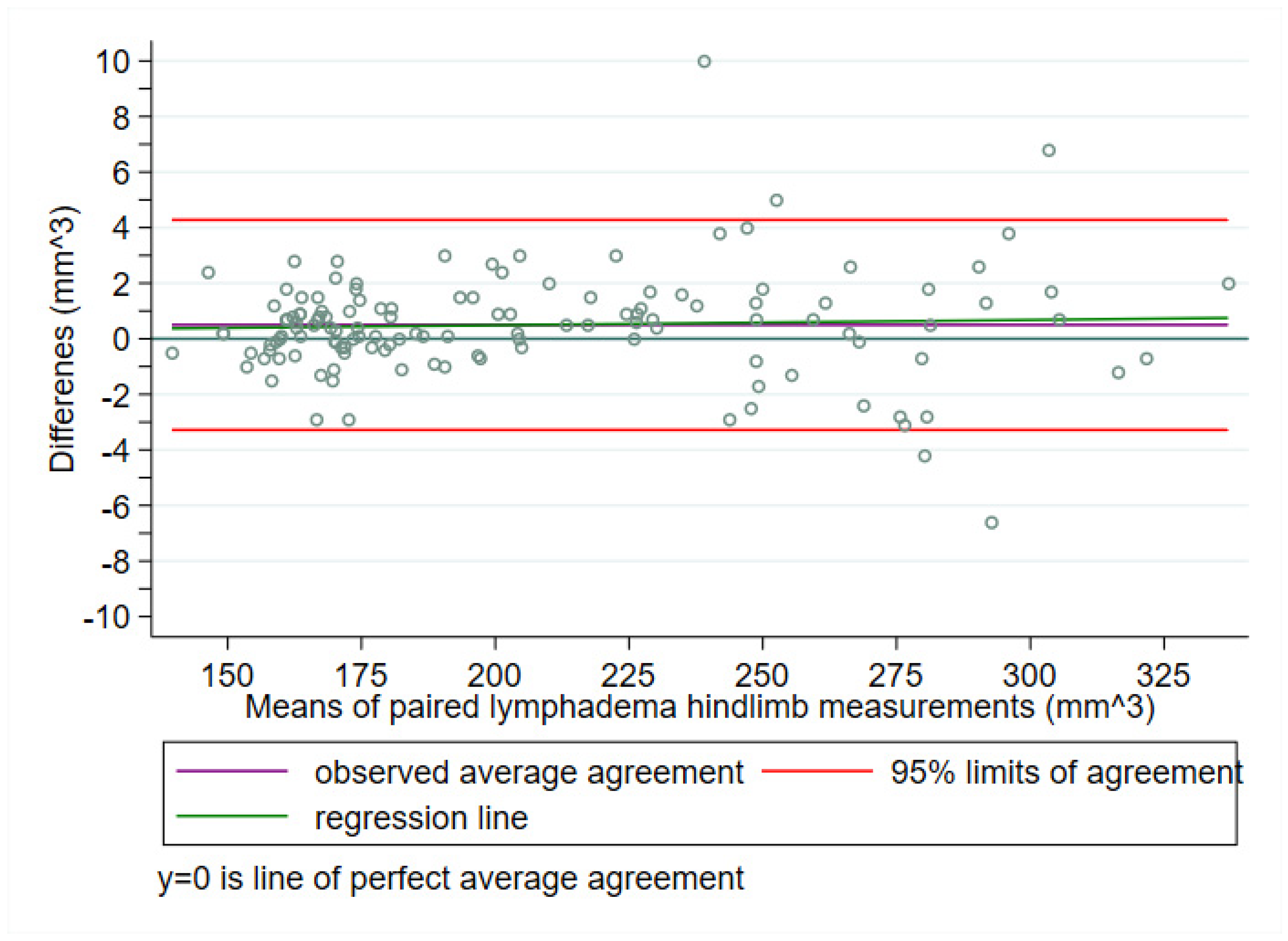
3.1. Frequentist Bland–Altman Analysis

3.1.1. Prediction Interval for a Future Difference

With α = 0.05 and n = 131, the prediction interval for a future observation was assessed as

$$PI=\overline{d}\pm t_{1-\frac{\alpha }{2};n-1}\sqrt{\frac{n+1}{n}}\times \widehat{\sigma }=0.50\pm 1.978\sqrt{\frac{132}{131}}\times 1.93=\left[-3.33;4.33\right].$$

(1)

This prediction interval spans marginally wider than the estimates for the LoA ${\hat{\mathsf{\theta }}}_1=-3.28$ and ${\hat{\mathsf{\theta }}}_2=4.28$ (see short dashes in Figure 2).

3.1.2. Outer 95% Confidence Limits for the LoA (i.e., θ₁ and θ₂)

For n = 131, $c_{OCI}$ equals 2.2404 according to Carkeet’s Supplemental Data S2 [6]. Hence,

$$OCI=\overline{d}\pm c_{OCI}\times \widehat{\sigma }=0.50\pm 2.2404\times 1.93=\left[-3.82;4.82\right].$$

(2)

These outer 95% confidence limits for the LoA span remarkably wider around the LoA ${\hat{\mathsf{\theta }}}_1=-3.28$ and ${\hat{\mathsf{\theta }}}_2=4.28$ as they quantify the outwards uncertainty around θ₁ and θ₂ (see long dashes in Figure 2).

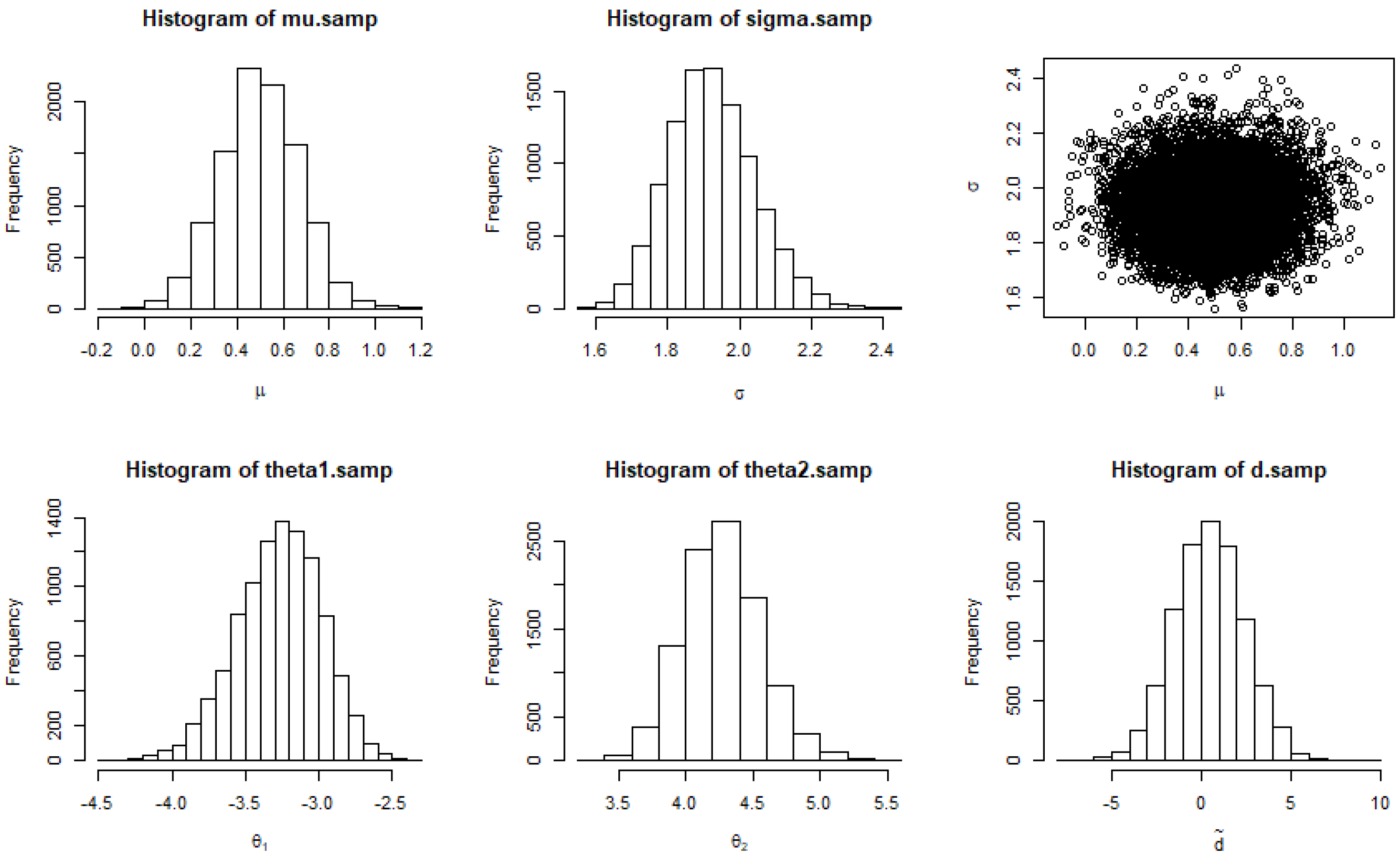
3.2. Bayesian Bland–Altman Analysis

3.2.1. Posterior Probability of a Future Difference $\tilde{d}$ Being in (−δ, δ)

After observing the differences D_i, i = 1,…,131, the posterior predictive distribution of a future difference is given in Figure 3 (bottom panel, right-hand side). We are, thus, 95% sure that a future difference will be between −3.30 and 4.27, i.e., the 95% Bayesian (posterior) predictive interval spans from −3.30 to 4.27 (see 0.025 and 0.975 quantiles of $\tilde{d}$ in

Table 2. Mean values; first, second, and third quartiles; and 0.025, 0.05, 0.95, and 0.975 quantiles of the posterior distributions of µ, σ, θ₁, θ₂ and of the posterior predictive distribution of a future difference (output from Supplemental Material Code S3).

Variable	Mean	2.5%	5%	Q1	Median	Q3	95%	97.5%
µ	0.50	0.17	0.23	0.39	0.50	0.61	0.77	0.83
σ	1.92	1.71	1.74	1.84	1.92	2.00	2.13	2.18
θ1	−3.26	−3.87	−3.76	−3.45	−3.25	−3.07	−2.82	−2.74
θ2	4.27	3.74	3.82	4.07	4.26	4.46	4.77	4.87
$\tilde{d}$	0.49	−3.30	−2.69	−0.76	0.48	1.80	3.68	4.27

). Further, we believe that a future difference will be within (−δ, δ) = (−5, 5) with a probability of 0.9880 (see post.pred.agree in the output from Supplemental Material Code S3).

3.2.2. Posterior Probability of H₁: θ₁ > −δ and θ₂ < δ

Figure 3 contains the posterior distribution of µ, σ, (µ,σ), and the LoA, θ_1, and θ₂. For example, the posterior mean of µ was 0.50, and the 95% credibility interval was [0.17; 0.83], Table 2. Likewise, the posterior mean and the 95% credibility interval was −3.26 and [−3.87; −2.74] for θ₁ and 4.27 and [3.74; 4.87] for θ₂. The posterior probability of H₁: θ₁ > −5 and θ₂ < 5 was 0.9895 (see post.h1 in the output from Supplemental Material Code S3). This probability corresponds to the proportion of combinations of (µ,σ) in Figure 3 (top panel, right-hand side) that fall within the ROPE which is the triangle (−5, 0), (0, 2.55), and (5, 0) here.

4. Discussion

The frequentist prediction interval was [−3.33; 4.33], and the outer 95% confidence limits for the LoA were −3.82 and 4.82. According to the Bayesian analysis, the equal-tailed 95% Bayesian (posterior) predictive interval was [−3.30; 4.27], and a future difference will be within (−δ, δ) = (−5, 5) with a probability of 0.9880. Outer credibility limits for the LoA were −3.87 and 4.87, with a posterior probability of the alternative hypothesis H₁: θ₁ > −5 and θ₂ < 5 that equaled 0.9895. The frequentist prediction interval for a future difference and its Bayesian counterpart, i.e., the Bayesian (posterior) predictive interval, were very close to each other, as were the frequentist outer 95% confidence limits and the Bayesian outer 95% credibility limits. The Bayesian results are accompanied by probabilistic statements on a future difference being within predefined benchmark values (−δ, δ) on the one hand and on the alternative hypothesis that the LoA fall within (−δ, δ) on the other hand.

4.1. Predicting One Future Difference versus Targeting the LoA

A prediction interval for a future difference, or a Bayesian (posterior) predictive interval for it, for that matter, may give an indication but appears clinically to be much less interesting than outer 95% confidence or credibility intervals of the LoA themselves. In practice, the focus will typically be on many future differences, not just on one. In terms of frequentist analysis, Vock [26] argued in favor of outer confidence limits for the LoA as these include the 2.5% and 97.5% target percentiles with a sufficiently high probability. In a Bayesian context, Alari, Kim, and Wand [25] reckoned that the researcher’s question of interest is of vital importance for whether one future difference or the LoA themselves are targeted. From our point of view, a sufficiently accurate estimate for the LoA is clearly preferred as a stronger case is built, be it in favor of or against method agreement.

4.2. Confidence versus Credibility

Frequentist and Bayesian thinking of what probability constitutes differ fundamentally: The frequentist view defines the probability of some event in terms of the relative frequency with which the event tends to occur, whereas the Bayesian view defines probability in more subjective terms, namely as a measure of the strength of your belief regarding the true situation [31,32].

Frequentist analysis assumes parameters to have exact but unknown values for which confidence intervals quantify the uncertainty of respective estimates based on observed data. Ninety-five percent confidence intervals are long-term statements in the way that 95% of the confidence intervals derived from many different samples from the same target population will comprise the true but unknown population parameter. A single 95% confidence interval will or will not include the true value, but with many possible samples in mind, one may argue that a specific 95% confidence interval stands a 95% chance of containing the true but unknown value (namely across all possible samples). Kruschke [27] (p. 318) reckons that the description of 95% confidence intervals as range of nonrejectable parameter values in null hypothesis significance testing is the most general and coherent one. To this end, a confidence interval is merely a range limited by two end-points, and it does not indicate any sort of probability distribution over values for the unknown parameter [27] (p. 323).

In Bayesian analysis, an unknown parameter is described by a distribution of possible values, not only by a single, unknown value to be estimated as in the frequentist setting. Prior beliefs about a parameter’s distribution are updated by newly gathered data, resulting in the posterior belief of that parameter’s distribution. In other words, credibility is reallocated across possibilities based on new data [27] (p. 15). Bayesian credibility intervals have three advantages over frequentist confidence intervals [27] (p. 324):

• Credibility intervals have a direct probabilistic interpretation in terms of the credibility of possible parameter values which confidence intervals do not have;
• Credibility intervals have no dependence on the sampling and testing intentions of the experimenter. Frequentist confidence intervals tell us about probabilities of data relative to imaginary possibilities generated from the experimenter’s intentions (namely the range of nonrejectable parameter values in null hypothesis significance testing, which focuses on the probability of observing the data as seen or data favoring the alternative hypothesis H₁, given H₀ were true);
• Credibility intervals are responsive to the experimenter’s prior belief based, for instance, on previous literature findings. Bayesian analysis indicates how much newly gathered data should alter our beliefs. Frequentist confidence intervals do not incorporate prior knowledge.

4.3. Group-Sequential Testing

Group-sequential testing and, more general, adaptive design methodology are well-developed and widely applied in clinical drug development [33,34,35,36,37,38], but to a much lesser extent in diagnostic research [39,40,41]. Zou et al. [42] employed the α-spending function approach [43,44,45] in connection with receiver operating characteristic curve analysis. Gerke et al. [46] exemplified analogously rater variability analysis with post-hoc interim analyses on the standard deviation σ. They supplemented corresponding upper one-sided confidence limits for σ, which can be used for decision making at an interim analysis time point instead of comparing the p-value at interim with the respective benchmark p-value according to the employed α-spending function. In the same way are outer confidence intervals for θ₁ and θ₂ constructed for confidence levels different from 95% which, in turn, correspond to hypothesis testing of H₀: θ₁ ≤ −δ or θ₂ ≥ δ against H₁: θ₁ > −δ and θ₂ < δ at significance levels smaller than 5% at interim analysis. To this end, Carkeet’s MATLAB code of his Supplemental Data S2 is a tool to derive exact confidence intervals for confidence levels different from 95% [6].

Similarly, Zhu and Yu [47] have proposed the application of α-spending functions in Bayesian analysis recently, and Kruschke [27] (pp. 383–392) exemplified various Bayesian strategies based on p-values, Bayes’ factor, credibility intervals’ length, and ROPEs. Any sequential testing strategy based on hypothesis testing—be it frequentist or Bayesian—may produce biased estimates as a result of stopping after observing extreme values up to an interim analysis time point. Therefore, he proposed to shift the focus to stopping when sufficient precision is achieved, for instance, in terms of the width of credibility intervals.

Stallard et al. [48] compared Bayesian and frequentist group-sequential tests when data can be summarized by normally distributed test statistics. Despite conceptual differences in frequentist and Bayesian analysis, Bayesian and frequentist group-sequential tests can have identical stopping rules in a single-arm trial or two-arm comparative trial with a prior distribution specified for the treatment difference. For instance, restricting Bayesian critical values at different interim analyses to be equal, O’Brien and Fleming’s design [44] corresponds to a Bayesian design with an exceptionally informative negative prior, and Pocock’s design [43] is an analogue to a Bayesian design with a non-informative prior.

4.4. Nonparametric Alternatives

Whenever the assumption of normally distributed differences does not hold, a non-parametric alternative analysis for the LoA is needed. Bland and Altman [3] proposed two methods. The former comprised the calculation of the proportion of differences exceeding some predefined benchmark values and comparing these to predefined acceptability limits. The latter represented nonparametric quantile estimation on the 2.5% and 97.5%, or, alternatively, on the 5% and 95% percentiles in small samples. Frey, Petersen, and Gerke [49] compared sample, subsampling, and kernel quantile estimators, as well as other methods for quantile estimation in small to moderate sample sizes (30 ≤ n ≤ 150). A simple sample quantile estimator (in the form of a weighted average of the observations closest to the target quantile), the Harrell–Davis estimator, and estimators of the Sfakianakis–Verginis type outperformed 10 other quantile estimators in terms of mean coverage for the next observation. These results were later confirmed when targeting the coverage probability of nonparametric LoA, and the three estimators above performed identically well for sample sizes of n ≥ 150 [50].

Nonparametric Bayesian LoA is a topic of future research [51,52,53].

4.5. Simplicity versus Interpretability

The inherent simplicity of the classical frequentist LoA has not only led to widespread adoption in the literature but also to a heterogeneous reporting of agreement assessments. There are numerous examples of when agreement analysis was equaled with reporting just sheer point estimates for the LoA whereas the interpretation of 95% outer confidence limits for the LoA reflects upon the uncertainty of the estimated values of the LoA. In comparison, a frequentist confidence interval represents merely a range of nonrejectable values for null hypothesis significance testing of H₀: θ₁ ≤ −δ or θ₂ ≥ δ against the alternative H₁: θ₁ > −δ and θ₂ < δ, Bayesian analysis allows for direct interpretation of both the posterior probability of the alternative hypothesis H₁ and the likelihood of parameter values.

The historical computational burden of Bayesian analysis has in the meantime been resolved; however, the solicitation of prior information and its implementation still requires thoughtful engagement. To use prior literature evidence to full capacity is, of course, appealing for efficacy and economic reasons, but requires careful balancing by weakening priors to account for, say, differences in inclusion and exclusion criteria between a previous study and the one that builds on the prior findings. In our example, for instance, the mean difference and the SD were clearly larger in study 2 than in study 1, despite identical experimental set-ups (including the very same raters) in our preclinical laboratory. Even if every effort is taken to rebuild the original study set-up, such inter-study differences may be observed within the very same research institution. The issue of securing comparable study designs, making the employment of prior information from another study reasonable and defensible, becomes much more challenging when combining study data from different research groups. For instance, Dykun and colleagues reported intra- and interrater reproducibility for left ventricle size quantification using non-contrast-enhanced cardiac computed tomography by means of intraclass correlation coefficients but did not give descriptive statistics for these comparisons [54]. Their data could possibly have been useful as prior information for one of our local studies [55], but the necessary information for doing so was simply not available to us.

Finally, our worked example was straightforward in terms of using per-subject data only. Incorporating correlated data (e.g., several lesions within the same patient) is well-established in frequentist Bland–Altman analysis [7], but requires more advanced hierarchical modelling in a Bayesian analysis of repeated measurement in method comparison studies [56].

References

1. Tukey, J.W. Exploratory Data Analysis; Pearson: Cambridge, MA, USA, 1977. [Google Scholar]
2. Altman, D.G.; Bland, J.M. Measurement in medicine: The analysis of method comparison studies. Statistician 1983, 32, 307–317. [Google Scholar] [CrossRef]
3. Bland, J.M.; Altman, D.G. Measuring agreement in method comparison studies. Stat. Methods Med. Res. 1999, 8, 135–160. [Google Scholar] [CrossRef] [PubMed]
4. Bland, J.M.; Altman, D.G. Statistical methods for assessing agreement between two methods of clinical measurement. Lancet 1986, 1, 307–310. [Google Scholar] [CrossRef]
5. Bland, J.M.; Altman, D.G. Agreed statistics: Measurement method comparison. Anesthesiology 2012, 116, 182–185. [Google Scholar] [CrossRef] [PubMed] [Green Version]
6. Carkeet, A. Exact parametric confidence intervals for Bland-Altman limits of agreement. Optom. Vis. Sci. 2015, 92, e71–e80. [Google Scholar] [CrossRef] [PubMed] [Green Version]
7. Olofsen, E.; Dahan, A.; Borsboom, G.; Drummond, G. Improvements in the application and reporting of advanced Bland-Altman methods of comparison. J. Clin. Monit. Comput. 2015, 29, 127–139. [Google Scholar] [CrossRef]
8. Webpage for Bland-Altman Analysis. Available online: https://sec.lumc.nl/method_agreement_analysis (accessed on 17 December 2021).
9. Jones, M.; Dobson, A.; O’Brian, S. A graphical method for assessing agreement with the mean between multiple observers using continuous measures. Int. J. Epidemiol. 2011, 40, 1308–1313. [Google Scholar] [CrossRef] [Green Version]
10. Christensen, H.S.; Borgbjerg, J.; Børty, L.; Bøgsted, M. On Jones et al.’s method for extending Bland-Altman plots to limits of agreement with the mean for multiple observers. BMC Med. Res. Methodol. 2020, 20, 304. [Google Scholar] [CrossRef]
11. Möller, S.; Debrabant, B.; Halekoh, U.; Petersen, A.K.; Gerke, O. An extension of the Bland-Altman plot for analyzing the agreement of more than two raters. Diagnostics 2021, 11, 54. [Google Scholar] [CrossRef] [PubMed]
12. Abu-Arafeh, A.; Jordan, H.; Drummond, G. Reporting of method comparison studies: A review of advice, an assessment of current practice, and specific suggestions for future reports. Br. J. Anaesth. 2016, 117, 569–575. [Google Scholar] [CrossRef] [Green Version]
13. Gerke, O. Reporting standards for a Bland-Altman agreement analysis: A review of methodological reviews. Diagnostics 2020, 10, 334. [Google Scholar] [CrossRef] [PubMed]
14. Taffé, P. When can the Bland & Altman limits of agreement method be used and when it should not be used. J. Clin. Epidemiol. 2021, 137, 176–181. [Google Scholar] [CrossRef]
15. Taffé, P. Assessing bias, precision, and agreement in method comparison studies. Stat. Methods Med. Res. 2020, 29, 778–796. [Google Scholar] [CrossRef] [PubMed]
16. Taffé, P.; Peng, M.; Stagg, V.; Williamson, T. MethodCompare: An R package to assess bias and precision in method comparison studies. Stat. Methods Med. Res. 2019, 28, 2557–2565. [Google Scholar] [CrossRef]
17. Taffé, P. Effective plots to assess bias and precision in method comparison studies. Stat. Methods Med. Res. 2018, 27, 1650–1660. [Google Scholar] [CrossRef] [PubMed]
18. Taffé, P.; Peng, M.; Stagg, V.; Williamson, T. biasplot: A package to effective plots to assess bias and precision in method comparison studies. Stata J. 2017, 17, 208–221. [Google Scholar] [CrossRef] [Green Version]
19. Choudhary, P.K.; Nagaraja, H.N. Measuring Agreement: Models, Methods, and Applications; Wiley: Hoboken, NJ, USA, 2017. [Google Scholar]
20. Carstensen, B. Comparing Clinical Measurement Methods: A Practical Guide; Wiley: Chichester, UK, 2010. [Google Scholar]
21. Shoukri, M.M. Measures of Interobserver Agreement and Reliability, 2nd ed.; Chapman & Hall: Boca Raton, FL, USA, 2010. [Google Scholar]
22. Dunn, G. Statistical Evaluation of Measurement Errors: Design and Analysis of Reliability Studies, 2nd ed.; Wiley: Chichester, UK, 2004. [Google Scholar]
23. Broemeling, L.D. Bayesian Biostatistics and Diagnostic Medicine; Chapman & Hall/CRC: Boca Raton, FL, USA, 2007. [Google Scholar]
24. Broemeling, L.D. Bayesian Methods for Measures of Agreement; Chapman & Hall/CRC: Boca Raton, FL, USA, 2009. [Google Scholar]
25. Alari, K.M.; Kim, S.B.; Wand, J.O. A tutorial of Bland Altman analysis in a Bayesian framework. Meas. Phys. Educ. Exerc. Sci. 2021, 25, 137–148. [Google Scholar] [CrossRef]
26. Vock, M. Intervals for the assessment of measurement agreement: Similarities, differences, and consequences of incorrect interpretations. Biom. J. 2016, 58, 489–501. [Google Scholar] [CrossRef]
27. Kruschke, J.K. Doing Bayesian Data Analysis, 2nd ed.; Academic Press/Elsevier: San Diego, CA, USA, 2015. [Google Scholar]
28. Bayesian Bland Altman Analysis. Available online: https://kalari.shinyapps.io/BBAA/ (accessed on 17 December 2021).
29. Wiinholt, A.; Gerke, O.; Dalaei, F.; Bučan, A.; Madsen, C.B.; Sørensen, J.A. Quantification of tissue volume in the hindlimb of mice using microcomputed tomography images and analysing software. Sci. Rep. 2020, 10, 8297. [Google Scholar] [CrossRef]
30. Bučan, A.; Wiinholt, A.; Dalaei, F.; Gerke, O.; Hansen, C.R.; Dhumale, P.; Sørensen, J.A. Validating lymphedema measurements in mice: Micro-CT scans, plethysmometer and caliper. 2021; in preparation. [Google Scholar]
31. Pezzullo, J.C. Biostatistics FD (For Dummies); Wiley: Hoboken, NJ, USA, 2013. [Google Scholar]
32. Bland, J.M.; Altman, D.G. Bayesians and frequentists. BMJ 1998, 317, 1151–1160. [Google Scholar] [CrossRef] [PubMed] [Green Version]
33. Whitehead, J. The Design and Analysis of Sequential Clinical Trials, 2nd ed.; Wiley: Chichester, UK, 1997. [Google Scholar]
34. Jennison, C.; Turnbull, B.W. Group Sequential Methods with Applications to Clinical Trials; Chapman & Hall/CRC: Boca Raton, FL, USA, 1999. [Google Scholar]
35. Jennison, C.; Turnbull, B.W. Adaptive and nonadaptive group sequential tests. Biometrika 2006, 93, 1–21. [Google Scholar] [CrossRef]
36. Todd, S. A 25-year review of sequential methodology in clinical studies. Stat. Med. 2007, 26, 237–252. [Google Scholar] [CrossRef] [PubMed]
37. Wassmer, G.; Brannath, W. Group Sequential and Confirmatory Adaptive Designs in Clinical Trials; Springer: New York, NY, USA, 2016. [Google Scholar]
38. Bauer, P.; Bretz, F.; Dragalin, V.; König, F.; Wassmer, G. Twenty-five years of confirmatory adaptive designs: Opportunities and pitfalls. Stat. Med. 2016, 35, 325–347. [Google Scholar] [CrossRef] [PubMed]
39. Zapf, A.; Stark, M.; Gerke, O.; Ehret, C.; Benda, N.; Bossuyt, P.; Deeks, J.; Reitsma, J.; Alonzo, T.; Friede, T. Adaptive trial designs in diagnostic accuracy research. Stat. Med. 2020, 39, 591–601. [Google Scholar] [CrossRef]
40. Vach, W.; Bibiza, E.; Gerke, O.; Bossuyt, P.M.; Friede, T.; Zapf, A. A potential for seamless designs in diagnostic research could be identified. J. Clin. Epidemiol. 2021, 129, 51–59. [Google Scholar] [CrossRef]
41. Hot, A.; Bossuyt, P.M.; Gerke, O.; Wahl, S.; Vach, W.; Zapf, A. Randomized test-treatment studies with an outlook on adaptive designs. BMC Med. Res. Methodol. 2021, 21, 110. [Google Scholar] [CrossRef] [PubMed]
42. Zou, K.H.; Liu, A.; Bandos, A.I.; Ohno-Machado, L.; Rockette, H.E. Statistical Evaluation of Diagnostic Performance: Topics in ROC Analysis; Chapman & Hall/CRC: Boca Raton, FL, USA, 2012. [Google Scholar]
43. Pocock, S.J. Group sequential methods in the design and analysis of clinical trials. Biometrika 1977, 64, 191–199. [Google Scholar] [CrossRef]
44. O’Brien, P.C.; Fleming, T.R. A multiple testing procedure for clinical trials. Biometrics 1979, 35, 549–556. [Google Scholar] [CrossRef]
45. Kim, K.; DeMets, D.L. Design and analysis of group sequential tests based on the type I error spending function. Biometrika 1987, 74, 149–154. [Google Scholar] [CrossRef]
46. Gerke, O.; Vilstrup, M.H.; Halekoh, U.; Hildebrandt, M.G.; Høilund-Carlsen, P.F. Group-sequential analysis may allow for early trial termination: Illustration by an intra-observer repeatability study. EJNMMI Res. 2017, 7, 79. [Google Scholar] [CrossRef] [Green Version]
47. Zhu, H.; Yu, Q. A Bayesian sequential design using alpha spending function to control type I error. Stat. Methods Med. Res. 2017, 26, 2184–2196. [Google Scholar] [CrossRef] [PubMed]
48. Stallard, N.; Todd, S.; Ryan, E.G.; Gates, S. Comparison of Bayesian and frequentist group-sequential clinical trial designs. BMC Med. Res. Methodol. 2020, 20, 4. [Google Scholar] [CrossRef] [PubMed]
49. Frey, M.E.; Petersen, H.C.; Gerke, O. Nonparametric limits of agreement for small to moderate sample sizes: A simulation study. Stats 2020, 3, 22. [Google Scholar] [CrossRef]
50. Gerke, O. Nonparametric limits of agreement in method comparison studies: A simulation study on extreme quantile estimation. Int. J. Environ. Res. Public Health 2020, 17, 8330. [Google Scholar] [CrossRef]
51. Hjort, N.L.; Holmes, C.; Müller, P.; Walker, S.G. Bayesian Nonparametrics; Cambridge University Press: New York, NY, USA, 2010. [Google Scholar]
52. Müller, P.; Quintana, F.A.; Jara, A.; Hanson, T. Bayesian Nonparametric Data Analysis; Springer: Cham, Switzerland, 2015. [Google Scholar]
53. Ghosal, S.; van der Vaart, A. Fundamentals of Nonparametric Bayesian Inference; Cambridge University Press: Cambridge, UK, 2017. [Google Scholar]
54. Dykun, I.; Mahabadi, A.A.; Lehmann, N.; Bauer, M.; Moebus, S.; Jöckel, K.H.; Möhlenkamp, S.; Erbel, R.; Kälsch, H. Left ventricle size quantification using non-contrast-enhanced cardiac computed tomography—association with cardiovascular risk factors and coronary artery calcium score in the general population: The Heinz Nixdorf Recall Study. Acta Radiol. 2015, 56, 933–942. [Google Scholar] [CrossRef]
55. Fredgart, M.H.; Lindholt, J.S.; Brandes, A.; Steffensen, F.H.; Frost, L.; Lambrechtsen, J.; Karon, M.; Busk, M.; Urbonavičiene, G.; Egstrup, K.; et al. Association of Left Atrial Size Measured by non-contrast Computed Tomography with Cardiovascular Risk Factors—The Danish Cardiovascular Screening Trial (DANCAVAS). Diagnostics 2018, submitted. [Google Scholar]
56. Schluter, P.J. A multivariate hierarchical Bayesian approach to measuring agreement in repeated measurement method comparison studies. BMC Med. Res. Methodol. 2009, 9, 6. [Google Scholar] [CrossRef] [Green Version]
Figure 1. Classical Bland–Altman plot including the estimated LoA and a regression line of the differences on the means.
Stats 04 00062 g001
Figure 2. Classical Bland–Altman plot including the estimated LoA and a regression line of the differences on the means, extended by a prediction interval for a future difference (short dashes) and exact outer 95% confidence limits for the LoA (long dashes).
Stats 04 00062 g002
Figure 3. The top panel shows the posterior distribution of µ, σ, and (µ,σ) from left to right. The bottom panel comprises the posterior distribution of θ1 and θ2 as well as the posterior predictive distribution of a future difference (from left to right; output from Supplemental Material Code S3).
Stats 04 00062 g003