1. Introduction and Background
This research follows up and provides new results on the performance of a previously described modified sandwich estimator [
1]. The intention was to address research gaps and to assess the suitability of this hybrid sandwich estimator, labeled the Rogers and Stoner estimator, for use with critical care data and to compare it to five other sandwich estimators. We assess the performance of the Rogers and Stoner estimator at different and greater degrees of correlation than previously performed. The assessment and comparison of this estimator to other sandwich estimators was done via simulation and real-world data. The question motivating our research involves the estimator’s performance during rare events, expressed as binary outcomes, in the critical care environment.
Longitudinal data is encountered frequently in many healthcare research areas, including the intensive care unit (ICU). Repeated measures from the same patient are expected to correlate with each other. The use of models with binary outcomes is not uncommon in this setting. Regression models for correlated binary outcomes are commonly fit using a generalized estimating equations (GEE) methodology. This project employed electronic health records (EHRs) from the Medical Information Mart for Intensive Care (MIMIC), a freely available ICU database that can support the examination of repeated measures within the critical-care ICU environment.
Available methods for use with independent data, such as logistic regression, are well known to most researchers. However, if the data is dependent, a method that accounts for the correlation is required. In situations with repeated or clustered measurements, researchers can employ GEE with dependent binary outcomes to account for the correlation within a covariance matrix. The correlation is a function of the covariance among the repeated or clustered measurements. GEE enables the investigator to specify the covariance structure based on the expected correlation pattern within the data. Its architecture employs a robust variance estimator, known as the sandwich estimator, that produces unbiased variance estimates for the regression coefficients if the sample is of adequate size [
2]. The advantage of the sandwich estimator is its estimation of unbiased standard errors, even when the covariance structure is misspecified. While this property benefits the GEE framework, the sandwich estimator of variance has some disadvantages.
The theoretical foundations of the sandwich estimator were established by Huber and expanded upon by White [
3,
4]. Liang and Zeger popularized the sandwich estimator by adapting it to GEE [
2]. Since that time, the sandwich, or robust estimator, has been a standard feature of most commercial statistical software packages and has become a staple of the GEE framework.
The asymptotic nature of the sandwich estimator is associated with problems when the sample size is small, or the outcome of interest is rare [
5,
6]. In small sample sizes, the sandwich estimator is biased downward and underestimates the variability of parameter estimators, which can lead to erroneous inferences. As a result, GEE Wald tests using the Liang and Zeger sandwich estimator produce p-values that are too small [
6]. Even in large samples, a rare outcome can produce issues much like the small-sample problem. The situation is aggravated further when both sample size is finite, and the outcome is rare.
When the data is independent, logistic regression models with binary outcomes underestimate the event’s probability when the outcome is rare [
7]. In these situations, Carroll et al. reported that the use of logistic regression, coupled with the sandwich estimator, produced an under-coverage of Wald-type tests [
5]. Furthermore, it was predicted that due to excess variability of the sandwich estimator in rare-event and small sample-size settings, this condition would result in an under-coverage of the confidence intervals. Diggle et al. stated, “… the robust approach is usually satisfactory when the data consists of short, essentially complete, sequences of measurements observed at a common set of times on many experimental units, and care is taken in the choice of a working covariance matrix” [
8]. As such, the purpose of this study is to showcase our proposed sandwich estimator along with others that exhibit better performance in these situations than that of the Liang and Zeger estimator.
2. Method
2.1. Generalized Estimating Equations and the Sandwich Covariance Estimator
Note that
Section 2.1 is repeated from our original publication and is included for the sake of completeness. In general, if
is a response variable and
is a covariate of interest for
subjects, a regression model can be utilized to describe their relationship. In the case of longitudinal data,
is the index for the number of observations within a given subject. The number of repeated measurements on an individual will be represented as
with
being the measurement at the
interval for the
subject. Marginal models are based on quasi-likelihood and are similar in form to the generalized linear model (GLM) in that a link function
is used to specify a mathematical relationship, involving regression coefficients
, between a marginal mean response
, and one or more independent variables
as indicated in Equation (1).
Regarding the GEE methodology, if
is a vector of predicted means for the
individual and
is the number of regression coefficients, then
where
will be used to represent the partial derivatives of the vector of predicted means with respect to the vector of regression coefficients
. Then
is an
matrix of these partial derivatives and appears as follows:
The variance (
) of the dependent variable (
) in the quasi-likelihood method, just as it is in GLM, can be expressed as a function (
) of the mean as indicated in Equation (2). Phi (
) is a scale parameter estimated from the data and is sometimes referred to as a nuisance parameter, as it is typically not of primary interest.
If is used to indicate the vector of outcomes for individual then let be the vector of variances for these effects. Let be a diagonal matrix that has taken on the values of the vector . Let represent the correlation within the clustered measurements then is the working correlation matrix for these same quantities. In this study, it is assumed that there is a correlation structure common to all subjects. If is an matrix with the variances of on the diagonal, then let indicate the working covariance matrix for these same measurements; depends on the correlation structure
In the GEE method, when the dependent variable comes from the exponential family, the following are the score equations for the regression coefficients
represented in Equation (3):
Liang and Zeger demonstrated that as the number of subjects or clusters (K) increased in size, that
is a consistent estimator for
[
2]. That is, as
is asymptotically multivariate Gaussian with zero mean and covariance matrix
estimated as follows.
Estimates of the partial derivatives of the vector of predicted means with respect to the vector of regression coefficients along with the working covariance matrix comprise . When estimates of and are inserted, is referred to as the empirical-based, or robust sandwich, variance matrix.
2.2. Review of Finite Sample Sandwich Estimators
Several approaches to improve the performance of the sandwich estimator over that of the Liang-Zeger in small sample sizes have been undertaken, including versions created by Pan, Morel, Mancl, and DeRouen as well as Rogers and Stoner [
1,
2,
9,
10,
11]. The Liang and Zeger, Mancl and DeRouen as well as the Rogers and Stoner sandwich estimators, sometimes will be referred to as Liang-Zeger, Mancl-DeRouen, and Rogers-Stoner, respectively. We provide a brief overview of these strategies for each approach, culminating in
Table 1, a listing of all sandwich estimators in vector-matrix notation.
Pan initially noted the superior performance of his modified sandwich estimator with exchangeable and independence covariance structures for both binary and continuous outcomes [
11]. His improved sandwich estimator utilized the pooled or average covariance-based upon all subjects. Hardin and Hilbe acknowledged the superiority of the Pan sandwich estimator over that of the Liang-Zeger in simulation studies [
12]. Our prior simulation work at low values of correlation confirmed their findings, and we sought to appraise the performance of Pan’s estimator at greater correlation values relative to the traditional Liang-Zeger as well as sandwich estimators by Rogers-Stoner, Morel, and Mancl-DeRouen [
1].
Mancl and DeRouen proposed a bias correction for the covariance of the original Liang-Zeger sandwich estimator. The bias adjustment subtracts
from the
identity matrix, in which
represents the naïve or model-based variance estimator listed in Equation (5) [
9]:
In his work with logistic regression for complex surveys, Morel proposed a correction in the Taylor series estimate of the covariance matrix to adjust for bias. This adjustment involved reintroducing an omitted term of the Taylor series estimate of the covariance matrix. This omitted term had very little effect on the covariance estimates until the sample or cluster size was reduced [
13]. Morel extended this concept to GEE for the sandwich estimator. In addition, he inflated this new sandwich estimator with the addition of a scaled version of the trace [
10]. Also, he suggested adding a scaled version of the determinant to the sandwich estimator, but never realized this alternate version. Our research included both of Morel’s sandwich estimators with the vector-matrix of the version inflated by the trace represented in
Table 1. Replacing trace with determinant in this vector-matrix equation results in the alternate version.
Rogers and Stoner proposed a hybrid sandwich estimator that used pooled covariances like Pan’s estimator and the addition of an inflation factor in the form of a scaled determinant similar to what Morel suggested [
1]. The determinant represents the volume of the variances and covariances of the sandwich estimator [
14]. The inflation factor is represented in Equation (6) and expresses the determinant in terms of the volume, where N is the total number of observations and p is the number of parameters as described in
Section 2.1.
The final form of this hybrid sandwich estimator is listed in
Table 1, along with the estimators by Liang-Zeger (1986), Pan (2001), Morel (2001), and Mancl-DeRouen (2003).
3. Prior Simulations and Discoveries
This research follows up prior work, which involved developing the methodology for and assessing the merits of a modified sandwich estimator for correlated binary outcomes in finite samples and rare-event data. Simulation studies with low correlation values in rare-event and finite data samples found this estimator performed better than the Liang-Zeger, Pan, Morel, and Mancl-DeRouen sandwich estimators. Sample sizes, prevalences, and covariance structures from these simulation settings are listed in
Table 2 [
1]. These simulation environments created coverage probabilities equivalent to a 95% confidence interval centered around the estimated regression coefficients. We discovered that when prevalence was lower than 30% and the sample size below 50 subjects, the choice of estimator mattered; the Liang-Zeger estimator consistently underestimated the coefficient variances. The Liang-Zeger estimator was the poorest performer in these settings, while the Rogers-Stoner and Pan estimators performed well, followed by the two Morel estimators. The Mancl-DeRouen also outperformed the Liang-Zeger sandwich estimator in this simulation environment. Due to the sandwich estimator’s asymptotic nature, it was not surprising that at sample sizes of 500 subjects, all sandwich estimators converged to 95% coverage probabilities.
4. Simulations
We followed up on our previous work and assessed the performance of the Rogers-Stoner estimator at different and greater degrees of correlation than had been done previously. We compared the performance of the Rogers-Stoner estimator to those developed by Liang-Zeger Pan, Morel, and Mancl-DeRouen, both in simulations and with real-world ICU data involving patients diagnosed with opioid poisoning. Again, as in our prior simulations, we used a balanced design with a single continuous covariate model fit on a series of simulated datasets having four repeated measures per subject with prevalences as high as 0.50 and as low as 0.01. The relationship between outcome prevalence and the correlation among longitudinal measures determined the choice of correlation settings; that is, the probability of the outcome restricted the range of possible correlation values [
6]. Differing sample sizes, outcome prevalences, and correlations varied as described in
Table 3. The compound symmetry covariance structure was omitted from the simulations, as an autoregressive structure was deemed more realistic for critical care repeated measures. The autoregressive correlation structure reflects correlation decay, with increasing intervals of time between measurements, and is considered practical, given the critical care study design.
Simulated correlated binary data was produced by the R-code library binarySimCLF developed by Qaqish [
15]. The standard deviation and average estimated standard error of the estimated regression coefficients were documented and recorded for each simulation. Each simulation configuration in
Table 3 was run 1000 times, retaining the average of each sandwich estimator. True values of
and regression coefficient
were set to one for all simulation tests. The single covariate
was normally distributed with a variance of one centered at a mean appropriate to the simulated prevalence
of the outcome. The relationship between the outcome prevalence and continuous covariate is described by:
Each sandwich estimator’s performance was assessed through 95% coverage probabilities for the regression coefficients. The simulation environment was programmed in the R version 2.11.1 statistical language [
16].
Coverage Probabilities
Performance of the sandwich estimators was assessed through coverage probabilities, which, as explained in our initial publication, was a better measure of performance than was the bias for the sandwich estimators. The coverage probability is the proportion of the time that the interval contained the true value of the regression coefficient. The coverage probabilities are similar to a confidence interval centered on the estimated regression coefficients; thus, they are a function of the estimated variance. The estimated variances for the regression coefficients were extracted from the diagonal of the sandwich estimator matrix. The simulation environment used the same estimated regression coefficients for each scenario and was designed to generate coverage probabilities similar to a 95% confidence interval.
5. Results
Simulation results, in terms of coverage probabilities, are presented for the independence covariance structures (
Figure 1 and
Figure 2) and the autoregressive covariance structures (
Figure 3). Figures are only shown for the
regression coefficient due to the similarity in results between
and
, the intercept. A composite figure is used for simulated outcome prevalence values of 5% through 10% under 0.01, 0.10, and 0.15 correlation with an autoregressive covariance structure. A single graph is dedicated to the 1% prevalence level under an independence structure in order to highlight differences in these extremely low prevalence conditions.
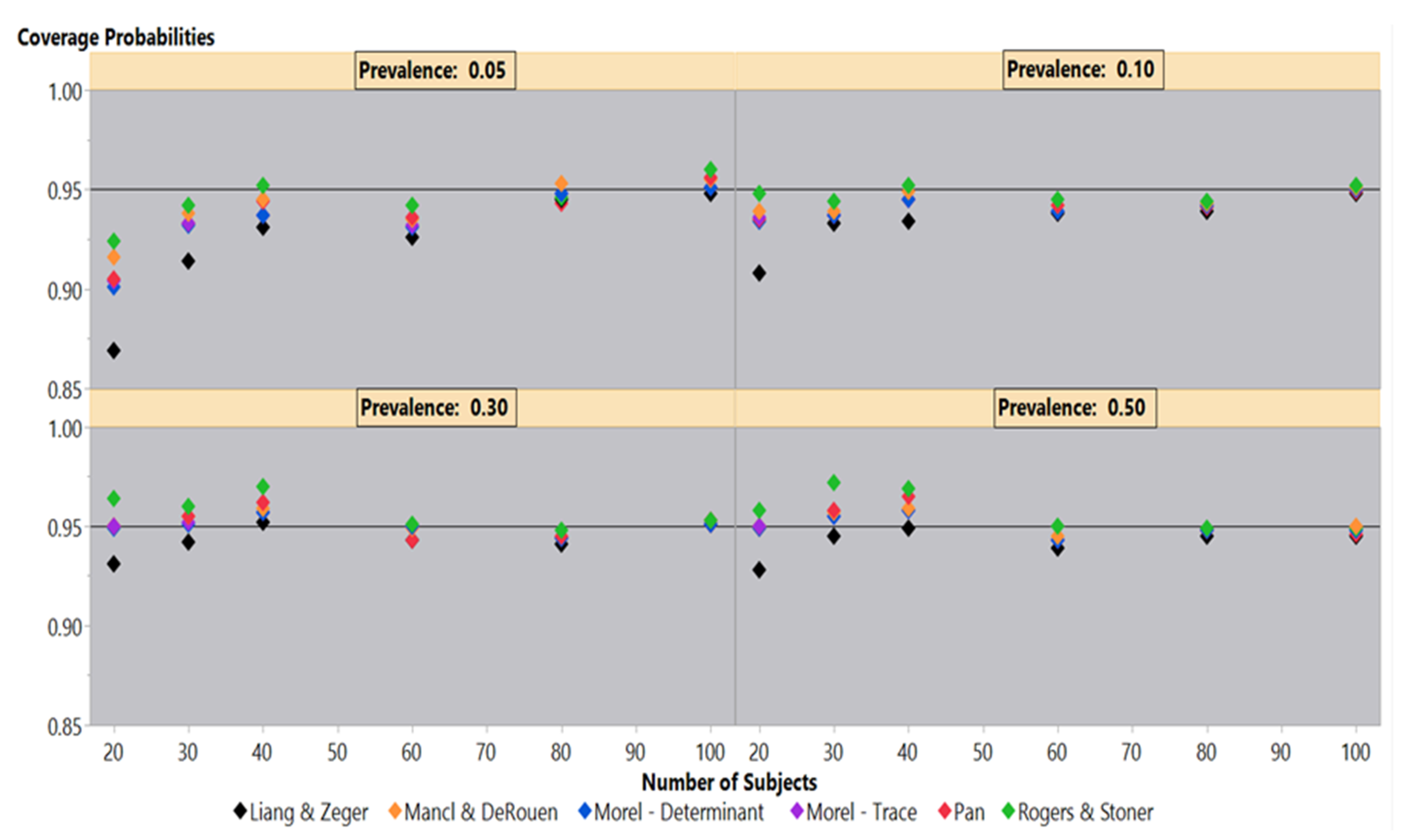
Simulations under an independence covariance structure for 50%–5% outcome prevalences illustrate the differences in coverage probability performance among the six sandwich estimators in
Figure 1. At 50% outcome prevalence, the Liang-Zeger maintains a roughly 95% coverage probability until 20 subjects, where it falls slightly lower than 95%. The remaining sandwich estimators also maintain a 95% coverage probability until 40 and 30 subjects, where they slightly overestimate the variances generating coverage probabilities larger than 95%. At 20 subjects, the Mancl-DeRouen, Pan, and both Morel estimators clearly are on the 95% coverage probability line, while the Rogers-Stoner is slightly above the 95% mark. The results under 30% mirror those under the 50% outcome prevalence, but to a lesser degree.
The 10% outcome prevalence shows that the Rogers-Stoner estimator maintains close to a 95% coverage probability, while the Pan, Mancl-DeRouen, and both Morel estimators marginally underestimate the variances; the coverage probabilities of the Liang-Zeger are well below the other five estimators at 20 subjects. Examining these sandwich estimators under the 5% outcome prevalence gives similar results until 30 and 20 subjects when all of the estimators are clearly below 95% coverage probabilities. At 20 subjects, the Liang-Zeger has declined to an 86.9% coverage probability, while the Rogers-Stoner estimator falls to 92.4%.
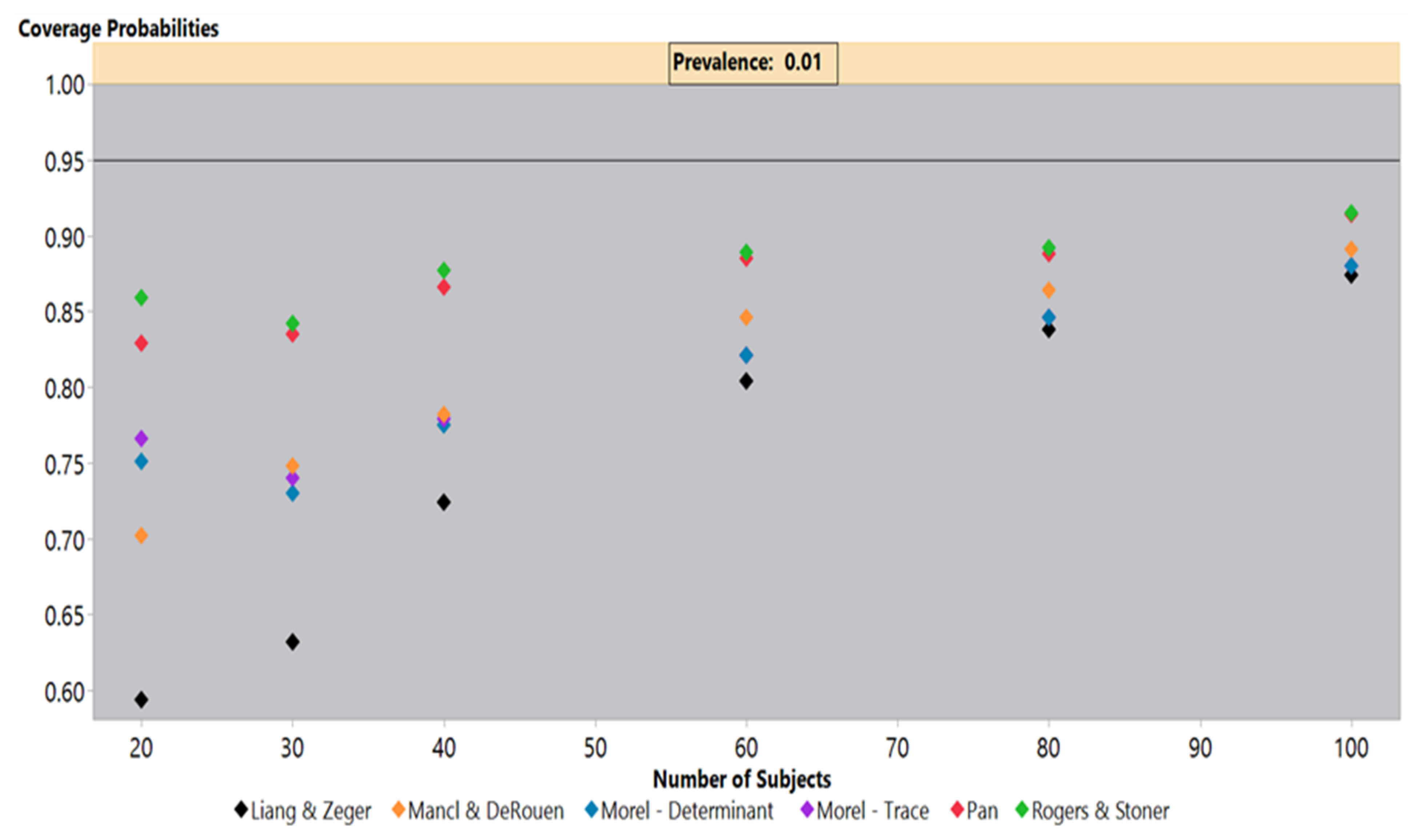
Simulations under an independence covariance structure with a 1% outcome prevalence, shown in
Figure 2, highlighted the coverage probability deficiencies under low prevalence settings for all sandwich estimators. The simulations indicated that even at 100 subjects, all estimators failed to achieve a 95% coverage probability, but the Pan and Rogers-Stoner estimators remained above 90%, while the Liang-Zeger had the poorest performance. The Liang-Zeger, or traditional sandwich estimator, demonstrated the greatest drop in coverage probabilities as the sample size decreased. At 20 subjects, the Liang-Zeger estimator’s coverage probabilities fell to under 60%, which is far below the other sandwich estimators. The coverage probabilities of the Mancl-DeRouen estimator also continued to decline as the sample size decreased, but it clearly outperformed the Liang-Zeger estimator. The Pan and Rogers-Stoner estimators’ performance was roughly steady from 80 to 40 subjects, but dropped slightly at 30, improving marginally at 20 subjects. We saw a similar performance from the two Morel estimators, but these lagged behind the Pan and Rogers-Stoner sandwich estimators.
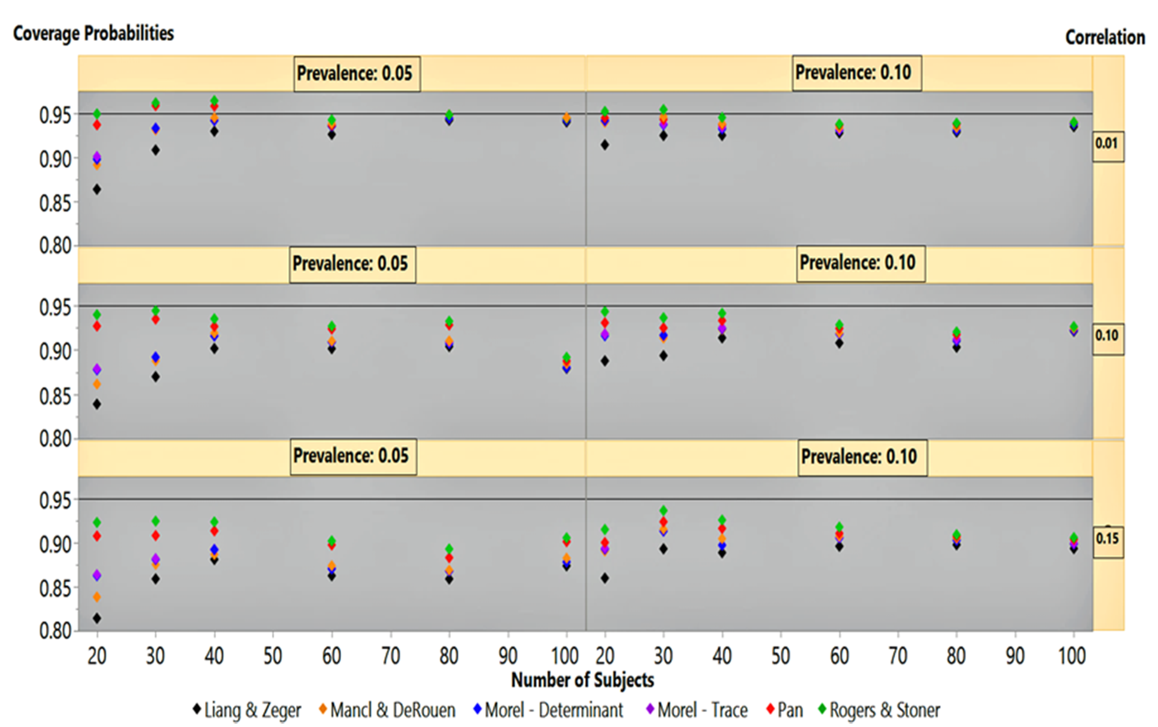
At outcome prevalences of 50% and 30%, under an autoregressive covariance structure, the estimators clustered around the 95% coverage probability line, except at 20 subjects (not shown). The Rogers-Stoner slightly overestimated the variances, although it varied slightly with the degree of correlation, while the Liang-Zeger clearly dipped below the 95% line. Performance of the sandwich estimators under an autoregressive correlation structure at 5% and 10% outcome prevalence is given in
Figure 3. It is not surprising that at the low correlation of 0.01, the estimators mirrored their performances in
Figure 1 for the independence covariance structure. This finding is similar to that in our previous simulation results under an autoregressive correlation structure with low correlation.
At 0.10 and 0.15 correlations,
Figure 3 shows that all estimators’ performance at 100 subjects had already dipped below the 95% coverage probability line. As the sample size decreased, the Rogers-Stoner sandwich estimator’s inflation term became significant, giving it a marginal edge over Pan’s estimator. The Liang-Zeger’s performance lagged behind all other sandwich estimators under 0.10 and 0.15 correlations, with 5% and 10% outcome prevalences as the sample size decreases. Performance of the estimators, under these two correlation settings, was similar between outcome prevalences within correlation strata, but differed by degree. The coverage probability results between the 0.10 and 0.15 correlation simulations mirrored one another, but the variances produced by all sandwich estimators under the 0.15 structure suffered a greater degree of underestimation, giving an exaggerated appearance in comparison to their 0.10 correlation structure counterparts.
6. Critical Care Application
In this Section, we discuss our use of MIMIC database version IV to compare the performance of the sandwich estimators in a real-world ICU setting. MIMIC-IV is an extension of MIMIC-III and contains the EHRs from patients in critical care units of the Beth Israel Deaconess Medical Center in Boston, Massachusetts, spanning the years 2008–2019 [
17]. The use of publicly available MIMIC ICU EHRs supports the reproducibility of our study [
18].
In the USA, ICU admissions related to opioid overdoses have increased by 34% over the last seven years [
19]. This rising epidemic has led to poisoning by opioids as the second leading cause of poisoning in the USA [
20]. Since the year 2000, the USA has experienced a 200% increase in opioid-related overdose deaths [
19]. A common symptom of acute opioid toxicity is respiratory depression, which may require the drug naloxone or some other respiratory intervention. Although many ICU patients diagnosed with opioid poisoning require some form of intervention to improve breathing, such as intubation or ventilation support, some patients in the MIMIC-IV ICU database did not require direct respiratory support.
The MIMIC-IV database stores ICU automated clinical system information and events logged manually by medical personnel. Within its tables, a code designates respiratory intervention procedures and includes descriptive text describing the intervention type. This study examined ICU patients diagnosed with opioid poisoning who did not undergo any procedure to improve respiration, such as ventilator support or intubation. Roughly 8% of these opioid-poisoned patients had a respiratory intervention code with descriptive text indicating they were repositioned to improve respiration. While in the ICU, these patients did not require any other ventilation support to improve respiration, although repositioning implies concerns over the patient’s ability to breathe. The MIMIC-IV emergency department module is not available to the public, so we could not determine if these patients had treatment or a procedure to improve respiration before ICU admission. It may be that ventilator support carried a greater risk, such as ventilator-associated pneumonia, than is warranted for patients who exhibited only mild respiratory depression symptoms. Also, the patient’s breathing may have been stable and regular at the time of ICU admission.
From the MIMIC-IV database, ICU EHRs, were randomly assigned to two groups consisting of 100 and 20 patients diagnosed with opioid poisoning who did not require any form of direct respiratory intervention while in the ICU. These group sizes corresponded to the largest and smallest samples from our simulations. Opioid poisoning was identified from the International Classification of Disease (ICD) versions 9 and 10 codes assigned to the patients’ EHRs. Heroin, an illicit drug continually increasing in popularity, was included in our ICD coding. The specific ICD codes included 965.00, 965.01, and 965.09 for version 9, while those for version 10 included the T40.0X, T40.1X, and T40.2X for poisoning by opium and heroin. These ICD codes for opioid-related overdoses were validated at the Beth Israel Deaconess Medical Center, functioning with a sensitivity and specificity of 100% [
19].
We used peripheral oxygen saturation (SpO2) as a measurement of the patient’s breathing effectiveness. This was automatically recorded by the iMDsoft Metavision ICU system and stored within the MIMIC database tables. We limited our examination of this sampling of patients to the first 24 h of ICU admission, constructing a longitudinal dataset of repositioning events and SpO2 measurements over the first 24 h of each patient’s stay. We studied four SpO2 measurements from each patient’s pulse oximeter readings over that 24 h. The first SpO2 measurement was randomly selected from the first six hours of the patient’s ICU stay, while the second was randomly selected from the sixth through the twelfth hours. The third SpO2 measurements were randomly selected between the twelfth and eighteenth hours, while the fourth SpO2 measurements were randomly selected between the eighteenth and twenty-fourth hours of the ICU patient’s stay.
If the patient was present in the ICU for fewer than 24 h, their stay was divided into four equal time intervals, with the SpO
2 measurements randomly drawn from these periods. When repositioning was performed, we randomly selected the SpO
2 measurement recorded in the following hour from the MIMIC database. We selected the following hour, as the act of repositioning a patient is logged manually, with the time recorded in the MIMIC-IV “chart time” database field. This field dates to an earlier period when paper charts were used to record notable patient events. These paper charts were divided into hourly blocks, and it was customary to log events at the top of the hour, a practice that has carried forward into the electronic era [
21]. By selecting the next hour, we ensured that the act of patient repositioning occurs before the SpO
2 reading. We hypothesized that repositioning alone, without any other respiratory intervention type, improves the patient’s breathing and is reflected in subsequent SpO
2 measurements.
GEE for Patient Repositioning Demonstration
The outcome event of interest was the act of repositioning a patient to improve respiration, represented as a binary variable; while the covariate of interest was the patient’s SpO
2 values, a continuous variable, recorded by the iMDsoft MetaVision ICU system and stored in the MIMIC-IV database table with its associated timestamp value. Repositioning was performed in 8.05% of the patients stricken with opioid poisoning within the first 24 h of ICU admission. The study question is represented by Equation (8), where
represents a binary outcome, with a one and zero indicating the occurrence or lack of a repositioning event, respectively. The symbol
represents the
patient while
signifies the first, second, third, or fourth six-hour interval of the patient’s ICU stay.
An autoregressive correlation structure reflects correlation decay with increasing intervals of time between measurements and was considered practical, given the design of the study. The six different sandwich estimators, covering four different time points for each patient, were used in this scenario with a test of significance performed on the
regression coefficient. The odds ratio is computed as the exponential function raised to the power of the regression coefficient. The p-value is the result of a hypothesis test of significance for the regression coefficient. The results of the sandwich estimators of variance, in samples of 100 and 20 subjects, are shown in
Table 4 and
Table 5, respectively.
Due to the asymptotic nature of the estimators and the large sample size of 100 subjects, the variances for
, shown in
Table 4, were close to the same size for all six sandwich estimators and the Z-scores indicate that there were no statistically significant results for any of the six sandwich estimators. Our first publication demonstrated that the coverage probabilities of the sandwich estimators will converge to the same value with a large enough sample size [
1]. At 100 subjects, the sandwich estimators are close to converging to the same value.
Results for the smaller sample size of 20 subjects, shown in
Table 5 had standard errors that differed significantly from each other. The six different estimators produced estimated variances for
of different magnitudes; the Liang-Zeger underestimated the variances while the Rogers-Stoner compensated with an inflation factor. The Liang-Zeger and both Morel estimators led to statistically significant results for
, while the Pan and Rogers-Stoner indicated statistically insignificant results. The Mancl-DeRouen estimator produced a borderline p-value but would have been considered statistically insignificant at a 0.05 level of significance. The estimated regression coefficient for a one-unit increase in SpO
2 in the sample of 20 subjects was −0.2712. If the results, in truth, had been statistically significant, the act of repositioning a patient would have worked to reduce respiration. The associated 95% odds ratio confidence interval for the Liang-Zeger and Rogers-Stoner sandwich estimators were (0.6583, 0.8828) and (0.4872, 1.1928), respectively.
These results highlighted that the choice of sandwich estimator for use in small sample sizes impacts the outcome of hypothesis testing regarding the regression coefficients. It is quite likely that repositioning opioid-poisoned patients was performed as a preventative measure rather than as a treatment for poor respiration. This would be one explanation for its lack of statistical significance in our model of 100 ICU patient subjects involving repositioning to improve respiration. It is also possible that the patients received treatment for respiratory depression in the emergency department and breathing stabilized before ICU admission. The MIMIC dataset includes an emergency department module that contains a record of these medications and treatments received by each subject, but this data is not publicly available.
7. Conclusions
This research further assessed the qualities of a hybrid sandwich estimator, reaffirming its superior performance over that of the Liang-Zeger estimator in simulations involving finite samples and low outcome prevalence. Furthermore, we demonstrated in simulations with sample sizes of 100 subjects and an autoregressive covariance structure with higher correlation settings (0.10 and 0.15) that all the sandwich estimators produced coverage probabilities that fell below 95%. This was not observed in our earlier simulations with low correlation values. As the sample sizes dropped under these same correlation conditions, the Liang-Zeger continued to perform abysmally while the Rogers-Stoner and Pan estimators adjusted. As the sample sizes decreased under a 0.10 correlation with 10% and 5% outcome prevalences, the coverage probabilities of the Liang-Zeger continued to deteriorate, while the Rogers-Stoner and Pan estimators recovered, almost achieving 95% coverage probabilities at 40 subjects and lower. In this situation, both Morel estimators were the next best performers, followed by the Mancl-DeRouen; the performance of the Liang-Zeger sandwich estimator finished well behind the Mancl-DeRouen at 20 subjects. As the correlation increased to 0.15 with a 10% outcome prevalence, the coverage probabilities of the Rogers-Stoner sandwich estimator achieved 94% coverage probabilities at 30 subjects, followed closely by the Pan at 92%. When the outcome prevalence dropped to 5% under 0.15 correlation, all of the sandwich estimators’ performances exhibited greater deterioration in comparison to the 0.10 correlation setting. Still, the Rogers-Stoner sandwich estimator, followed closely by the Pan estimator, logged superior performance in terms of coverage probabilities. In sample sizes of 20 subjects under a 0.15 correlation structure, the Rogers-Stoner and Pan sandwich estimators had 92% and 91% coverage probabilities, respectively.
The performance of the Liang-Zeger sandwich estimator, under an independence covariance structure at 50% and 30% outcome prevalences, did well until the sample size dropped to 20 subjects, while the Rogers-Stoner, Pan, Mancl-DeRouen, and both Morel estimators generated variances that were too large for the regression coefficient resulting in coverage probabilities greater than 95%. This overestimation of variances was greatest in the Rogers-Stoner sandwich estimator. With a 1% outcome prevalence and an independence covariance structure, the coverage probabilities of all the sandwich estimators were under 95% at 100 subjects and steadily declined as the sample size decreased. At 20 subjects, the Rogers-Stoner and Pan estimators improved slightly from their performance with 30 subjects. The sandwich estimators in order of best coverage probability performance at 20 subjects and 1% prevalence were: Rogers-Stoner (86%), Pan (83%), Morel (Trace—77%; Determinant—75%), Mancl-DeRouen (70%), and Liang-Zeger (59%).
In our previously published research on simulations involving only low values of correlation, we concluded that, as the outcome prevalence dropped below 30% and the sample size below that of 50 subjects, the choice of estimators matters, and alternatives to the Liang-Zeger estimator should be considered. In our limited simulation settings, the Rogers-Stoner sandwich estimator outperformed the Liang-Zeger and typically outperformed all other estimators as both the prevalence and sample size decreased [
1]. We further noted that the Rogers-Stoner estimator’s performance could be inferior compared to that of the Pan estimator under different correlation settings. The simulation results of this study demonstrated that the Rogers-Stoner sandwich estimator has a slight performance edge over the Pan sandwich estimator in settings of higher correlation (0.10 and 0.15), finite sample sizes, and low outcome prevalences of 5% and 10%.
The Rogers-Stoner and Pan sandwich estimators have similar performances because the former is an extension of the latter. The Rogers-Stoner estimator is dependent on a scaled version of the determinant in the inflation factor, similar to that in Morel’s description, to improve performance in situations with small sample sizes and low outcome prevalences.
In summary, the Liang-Zeger sandwich estimator’s performance suffered as the sample sizes dropped below 60 subjects under correlation settings as low as 0.01 when outcome prevalence values were less than 30%. This drop-off in performance was exacerbated further by lower outcome prevalence values, smaller sample sizes, and higher correlation settings (0.10 and 0.15). The observed results were congruent with Carroll and colleagues’ predictions [
5]. Under these extreme settings, the Rogers-Stoner and Pan estimators would be good choices for variance estimators, followed by either of the two estimators proposed by Morel.
The choice of a sandwich estimator is crucial in deriving correct statistical inferences. The real-world ICU practice of patient repositioning to improve opioid-induced respiratory depression showed the danger in hypothesis testing for low-prevalence situations with small sample sizes in GEE models with binary outcomes. Using data from MIMIC ICU EHRs, we demonstrated the limitations of the Liang-Zeger sandwich estimator with rare events and finite sample sizes. Sandwich estimators proposed by Rogers-Stoner, Pan, Morel, and Mancl-DeRouen could all serve as preferable alternatives to the traditional Liang-Zeger under these conditions.


