
Generalized Cardioid Distributions for Circular Data Analysis

 ,
, 

Abstract
:1. Introduction
2. Generalized Cardioid Models
- (a)
- The -G cdf defined by Eugene et al. [6] iswhere are two additional parameters, is the incomplete beta function ratio evaluated at , and is the complete beta function;
- (b)
- The Kw-G cdf pioneered by Cordeiro and Castro [8] iswhere are two additional parameters;
- (c)
- The -G cdf reported by Zografos and Balakrishnan [7] iswhere , is the gamma function, and is the incomplete gamma function;
- (d)
- The MO-G cdf defined by Marshal and Olkin [5] iswhere is a shape parameter.
- ;
- .
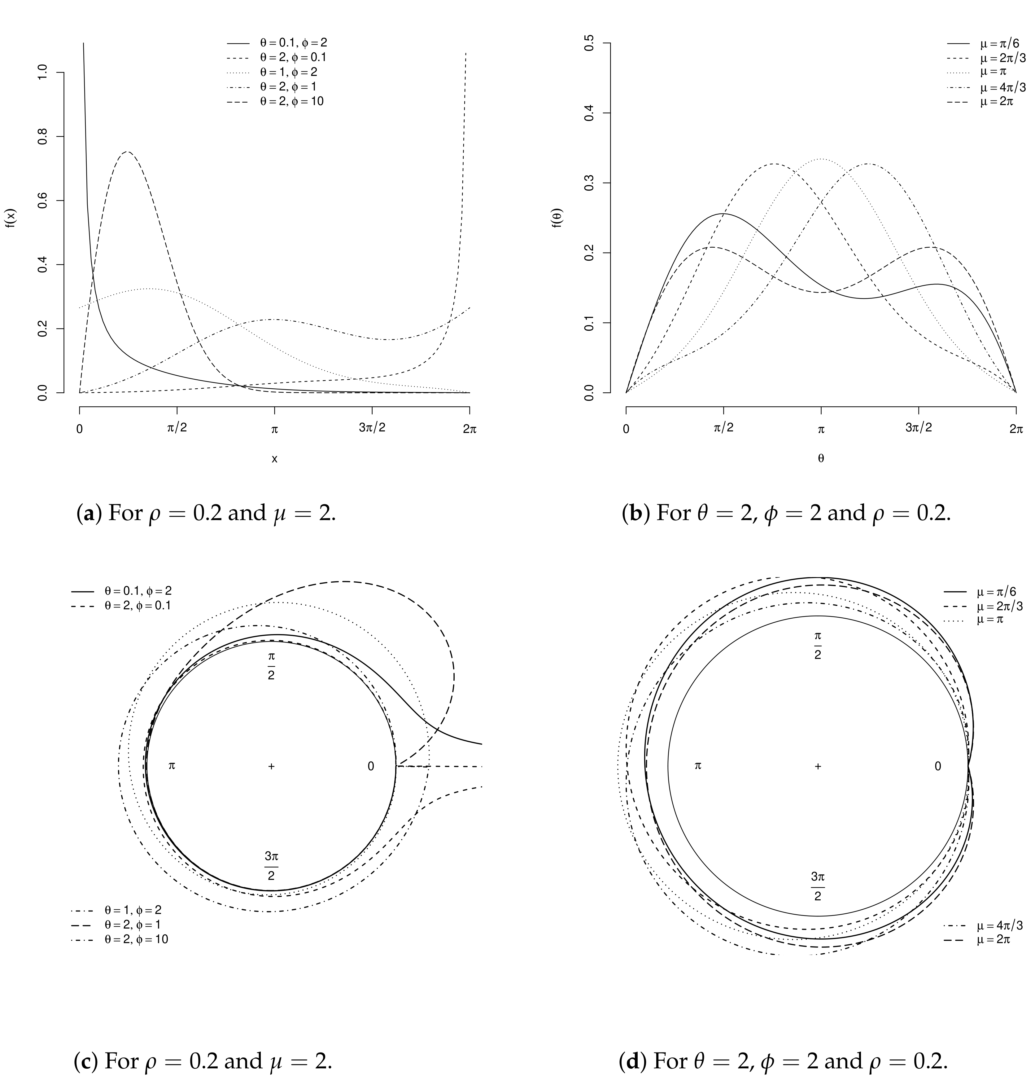
2.1. Beta Cardioid
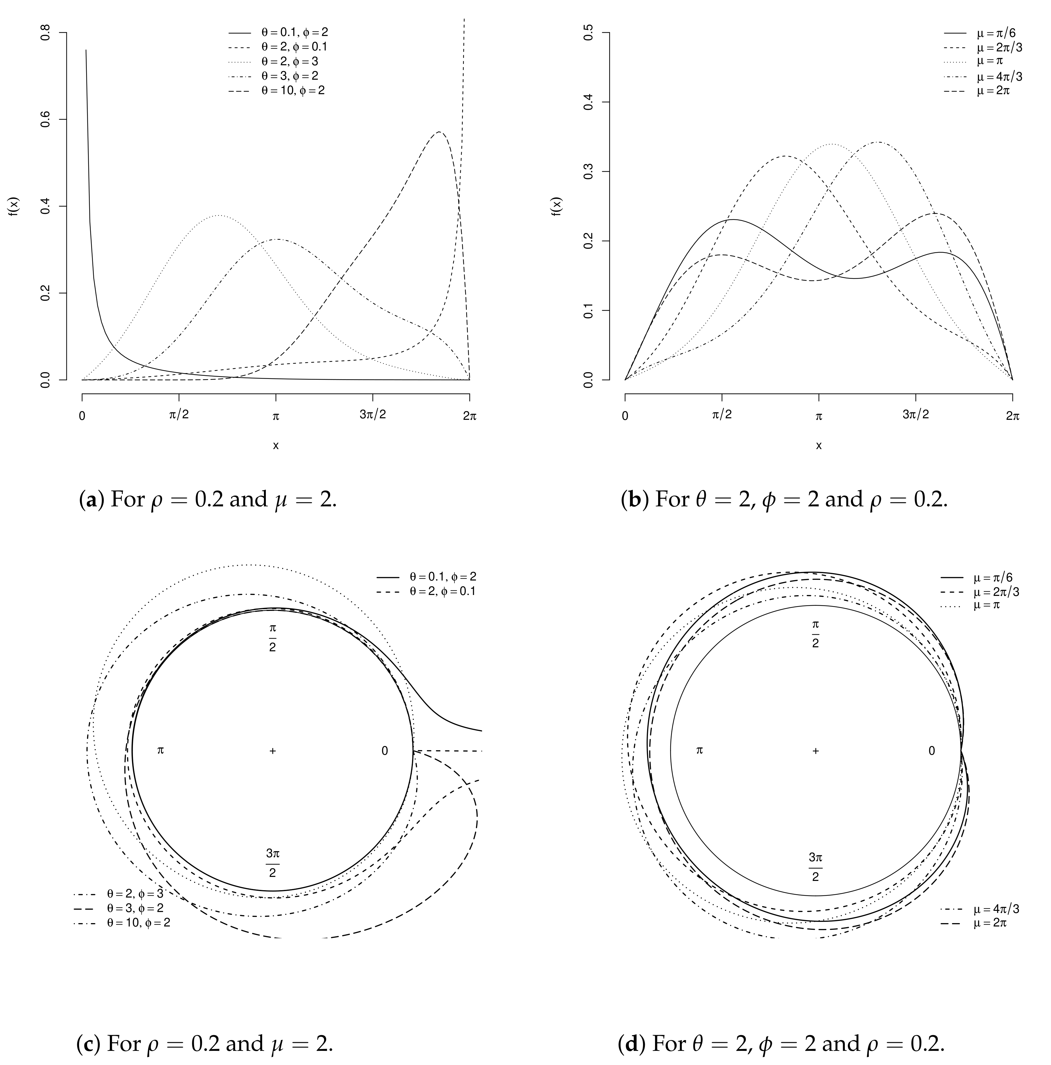
2.2. Kumaraswamy Cardioid
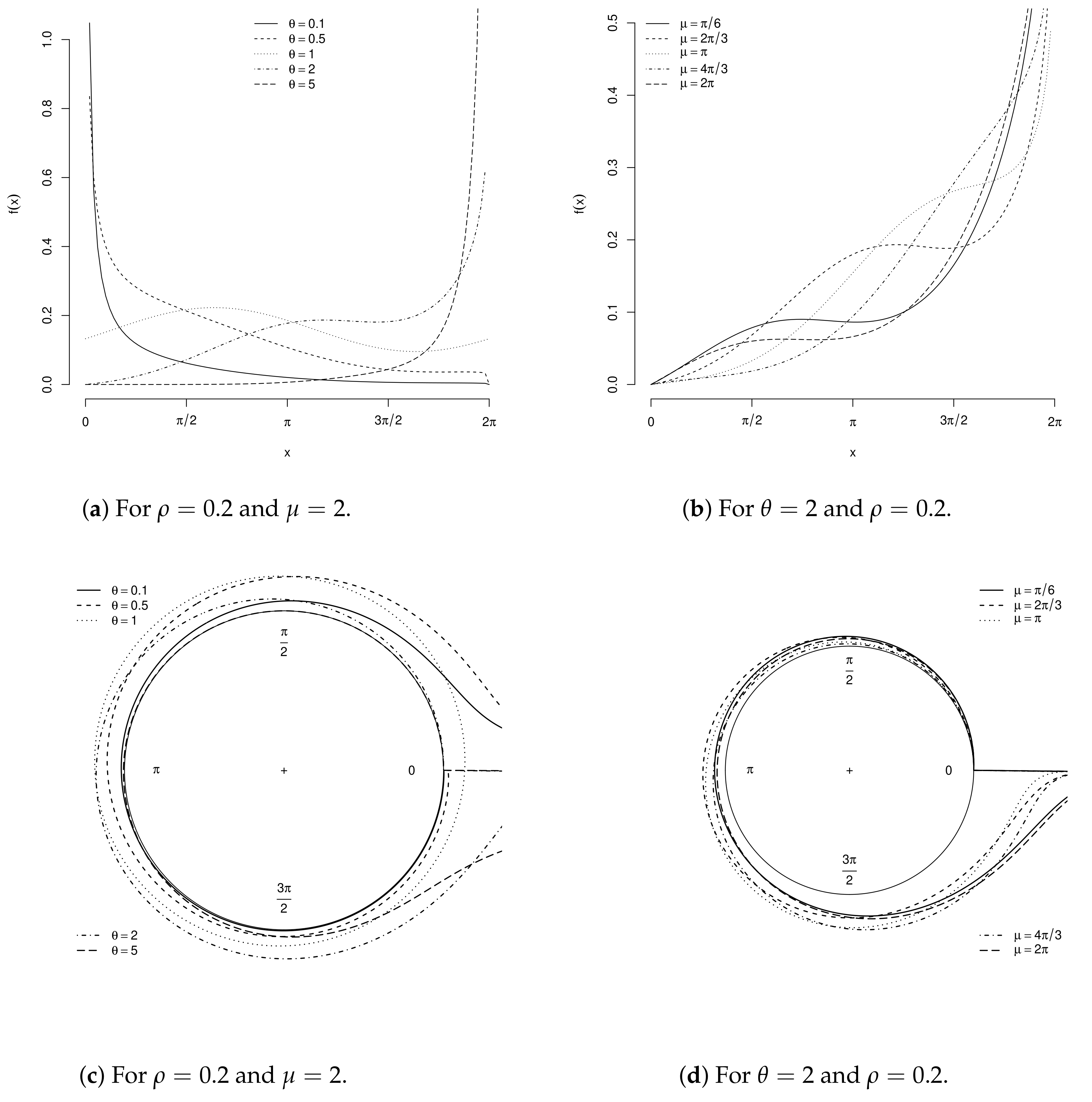
2.3. Gamma Cardioid
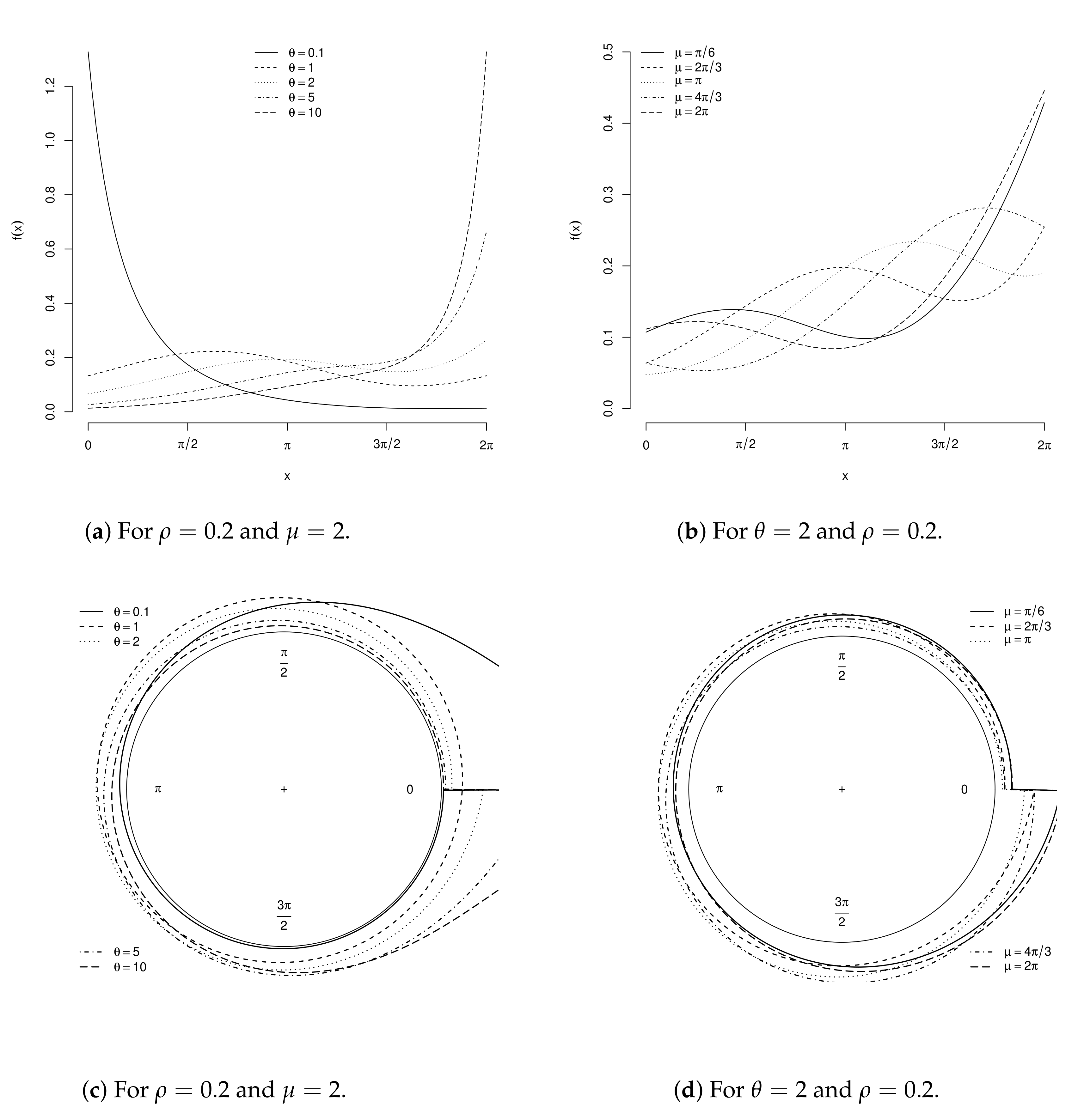
2.4. Marshall–Olkin Cardioid
2.5. A General Formula
3. Mathematical Properties
- From Nadarajah et al. [27]:
- From Cordeiro and de Castro [8]:
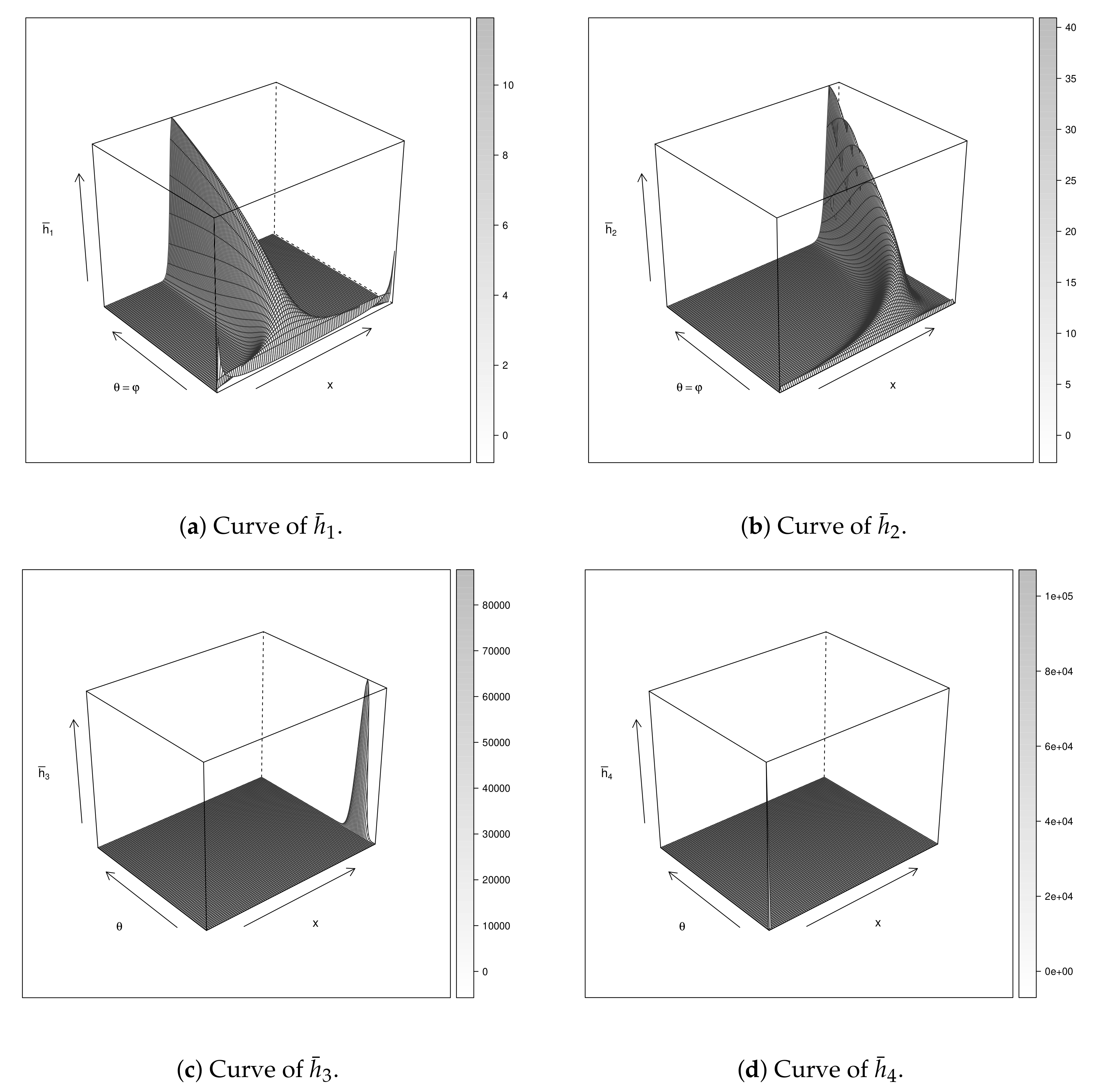
- From Paula et al. [18]:Let . The cdf of is (Paula et al., 2020)By simple differentiation, we can writewhere ,After some algebraic manipulations, the pth central circular trigonometric moment of , say , with mean direction , follows aswhere and . The functions and are easily handled both numerically and analytically.For example, Table 2 displays some special quantities using the symbolic computation software wxmaxima.
4. Estimation
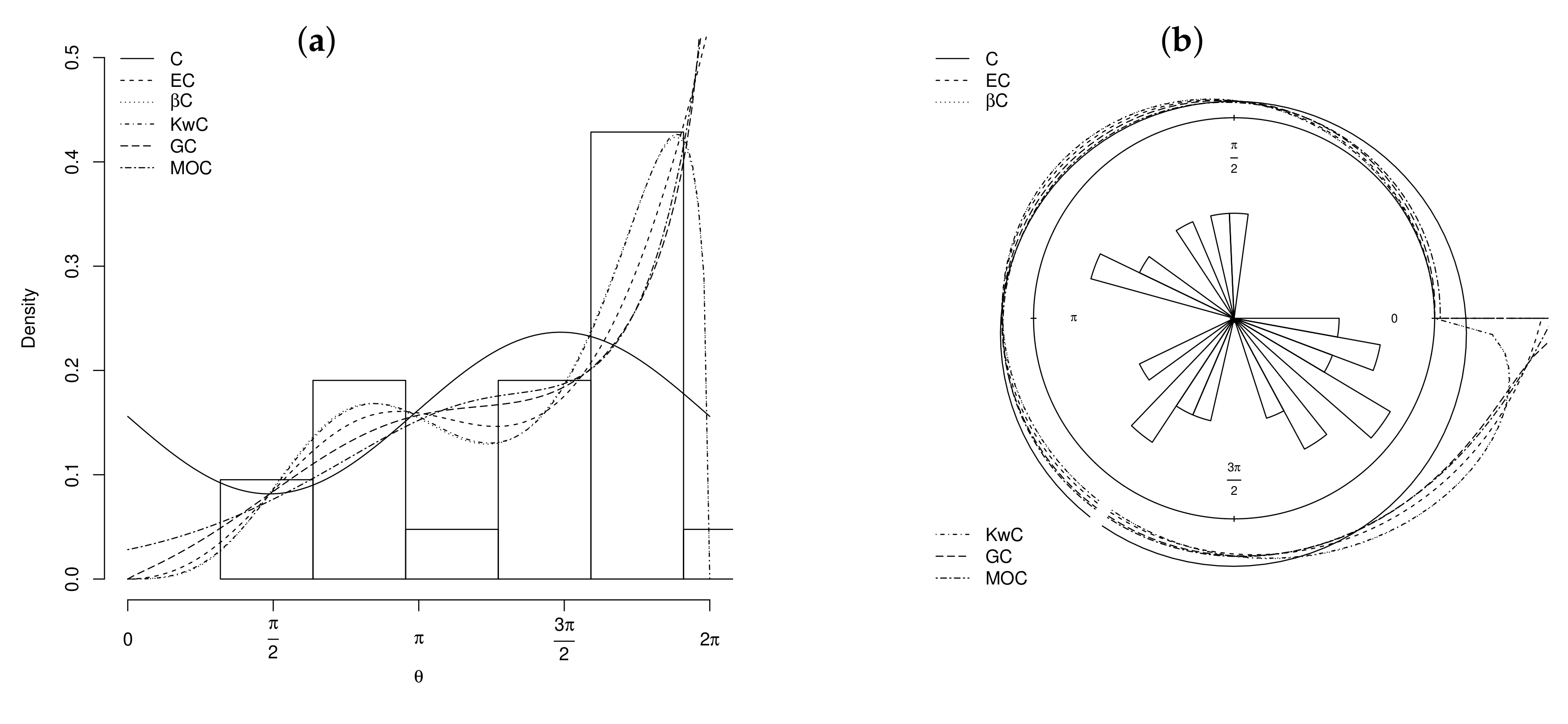
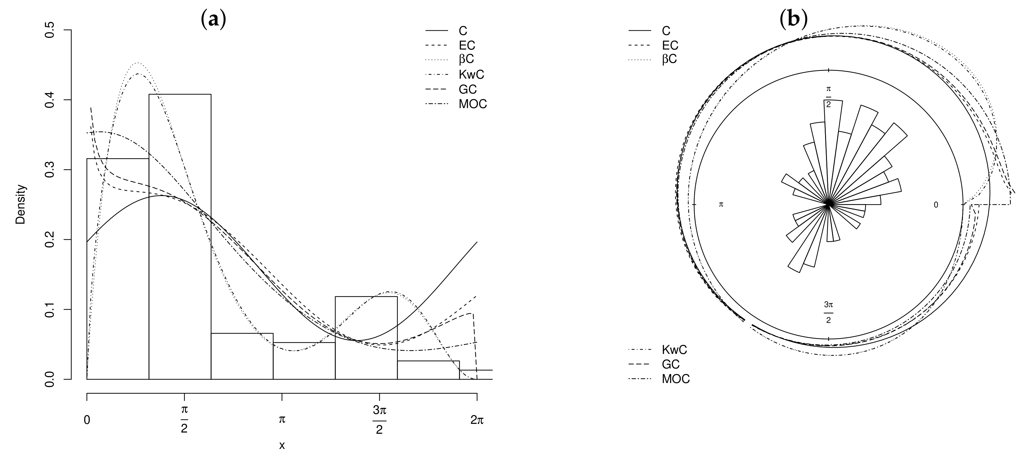
5. Applications
6. Conclusions
Author Contributions
Funding
Institutional Review Board Statement
Informed Consent Statement
Data Availability Statement
Conflicts of Interest
References
- Astfalck, L.C.; Cripps, E.J.; Gosling, J.P.; Hodkiewicz, M.R.; Milne, I.A. Expert elicitation of directional metocean parameters. Ocean Eng. 2018, 161, 268–276. [Google Scholar] [CrossRef]
- Broly, P.; Deneubourg, J.-L. Behavioural contagion explains group cohesion in a social crustacean. PLoS Comput. Biol. 2015, 11, e1004290. [Google Scholar] [CrossRef]
- García-González, A.; Damon, A.; River, F.B.; Gosling, J.P. Circular distribution of three species of epiphytic orchids in shade coffee plantations, in Soconusco, Chiapas, Mexico. Plant Ecol. Evol. 2016, 149, 189–198. [Google Scholar] [CrossRef]
- Gatto, R. Saddlepoint approximations to tail probabilities and quantiles of inhomogeneous discounted compound poisson processes with periodic intensity functions. Methodol. Comput. Appl. Probab. 2012, 14, 1053–1074. [Google Scholar] [CrossRef]
- Marshall, A.W.; Olkin, I. A new method for adding a parameter to a family of distributions with application to the exponential and Weibull families. Biometrika 1977, 84, 641–652. [Google Scholar] [CrossRef]
- Eugene, N.; Lee, C.; Famoye, F. Beta-normal distribution and its applications. Commun. Stat. Theory Methods 2002, 31, 497–512. [Google Scholar] [CrossRef]
- Zografos, K.; Balakrishnan, N. On families of beta-and generalized gamma-generated distributions and associated inference. Stat. Methodol. 2009, 6, 344–362. [Google Scholar] [CrossRef]
- Cordeiro, G.M.; Castro, M. A new family of generalized distributions. J. Stat. Comput. Simul. 2011, 6, 883–898. [Google Scholar] [CrossRef]
- Cordeiro, G.M.; Ortega, E.M.; Cunha, D.C. The exponentiated generalized class of distribution. J. Data Sci. 2013, 11, 1–27. [Google Scholar] [CrossRef]
- Cordeiro, G.M.; Alizadeh, M.; Marinho, P.R.D. The type I half-logistic family of distributions. J. Stat. Comput. Simul. 2016, 86, 707–728. [Google Scholar] [CrossRef]
- Yousof, H.M.; Afify, A.Z.; Hamedani, G.; Aryal, G.R. The Burr X generator of distributions for lifetime data. J. Stat. Theory Appl. 2016, 16, 288–305. [Google Scholar] [CrossRef] [Green Version]
- Cordeiro, G.M.; Afify, A.Z.; Yousof, H.M.; Pescim, R.R.; Aryal, G.R. The exponentiated Weibull-H family of distributions: Theory and applications. Mediterr. J. Math. 2017, 14, 155–176. [Google Scholar] [CrossRef]
- Lee, J.-S.; Hoppel, K.W.; Mango, S.A.; Miller, A.R. Intensity and phase statistics of multilook polarimetric and interferometric SAR imagery. IEEE Trans. Geosci. Remote Sens. 1994, 32, 1017–1028. [Google Scholar]
- Breckling, J. The Analysis of Directional Time Series: Applications to Wind Speed and Direction; Springer: Berlin/Heidelberg, Germany, 1989. [Google Scholar]
- Jeffreys, H. Theory of Probability; Oxford University Press: Oxford, UK, 1983. [Google Scholar]
- Wang, M.Z.; Shimizu, K. On applying Möbius transformation to Cardioid random variables. Stat. Methodol. 2012, 9, 604–614. [Google Scholar] [CrossRef]
- Abe, T.; Pewsey, A.; Shimizu, K. On Papakonstantinou’s extension of the Cardioid distribution. Stat. Probab. Lett. 2009, 79, 2138–2147. [Google Scholar] [CrossRef]
- Paula, F.V.; Nascimento, A.D.C.; Amaral, G.J.A. A new extended Cardioid model: An application to wind data. Submitt. J. Math. Imaging Vis. 2020. [Google Scholar]
- Jamal, F.; Chesneau, C.; Bouali, D.L.; Ul Hassan, M. Beyond the Sin-G family: The transformed Sin-G family. PLoS ONE 2021, 16, e0250790. [Google Scholar] [CrossRef] [PubMed]
- Souza, L.; Júnior, W.R.O.; Brito, C.C.R.; Chesneau, C.; Ferreira, T.A.E.; Soares, L.G.M. General properties for the Cos-G Class of Distributions with Applications. Eurasian Bull. Math. 2019, 2, 63–79. [Google Scholar]
- Abraham, C.; Molinari, N.; Servien, R. Unsupervised clustering of multivariate circular data. Stat. Med. 2013, 32, 1376–1382. [Google Scholar] [CrossRef] [PubMed] [Green Version]
- Qiu, X.; Wu, S.; Wu, H. A new information criterion based on langevin mixture distribution for clustering circular data with application to time course genomic data. Stat. Sin. 2015, 25, 1459–1476. [Google Scholar] [CrossRef]
- Jammalamadaka, S.R.; Sengupta, A. Topics in Circular Statistics; World Scientific Publishing: Singapore, 2001. [Google Scholar]
- Mardia, K.V.; Sutton, T.W. On the modes of a mixture of two von Mises distributions. Biometrika 1975, 62, 699–701. [Google Scholar] [CrossRef]
- Yilmaz, A.; Biçer, C. A new wrapped exponential distribution. Math. Sci. 2018, 12, 285–293. [Google Scholar] [CrossRef] [Green Version]
- Pewsey, A.; Neuhäuser, M.; Ruxton, G. Circular Statistics in R; Oxford University Press: Oxford, UK, 2013. [Google Scholar]
- Nadarajah, S.; Cordeiro, G.M.; Ortega, E.M. General results for the beta-modified Weibull distribution. J. Stat. Comput. Simul. 2011, 81, 1211–1232. [Google Scholar] [CrossRef]
- Castellares, F.; Lemonte, A.J. A new generalized weibull distribution generated by gamma random variables. J. Egypt. Math. Soc. 2015, 23, 382–390. [Google Scholar] [CrossRef] [Green Version]
- Cordeiro, G.M.; Lemonte, A.J.; Ortegam, E.M. The Marshall–Olkin family of distributions: Mathematical properties and new models. J. Stat. Theory Pract. 2014, 8, 343–366. [Google Scholar] [CrossRef]
- Casella, G.; Berger, R. Statistical Inference; Thomson Learning: Boston, MA, USA, 2002. [Google Scholar]
- Johnson, R.A.; Wehrly, T. Measures and models for angular correlation and angular-linear correlation. J. R. Stat. Soc. (Ser. B) 1977, 39, 222–229. [Google Scholar] [CrossRef] [Green Version]
- Stephens, M.A. Techniques for Directional Data; Stanford University: Stanford, CA, USA, 1969. [Google Scholar]
- Henningsen, A.; Toomet, O. maxlik: Package for maximum likelihood estimation in R. Comput. Stat. 2011, 26, 443–458. [Google Scholar] [CrossRef]

| Model | C | KwC | C | MOC | |
|---|---|---|---|---|---|
| Index (i) | • | 1 | 2 | 3 | 4 |
| Expression |
| Model | Kuiper | Watson | AIC | BIC | ||||
|---|---|---|---|---|---|---|---|---|
| C | − | − | ||||||
| () | () | − | − | |||||
| EC | − | |||||||
| − | ||||||||
| C | ||||||||
| () | () | () | () | |||||
| KwC | ||||||||
| () | () | () | () | |||||
| C | − | |||||||
| () | () | () | − | |||||
| MOC | − | |||||||
| () | () | () | − |
Publisher’s Note: MDPI stays neutral with regard to jurisdictional claims in published maps and institutional affiliations. |
© 2021 by the authors. Licensee MDPI, Basel, Switzerland. This article is an open access article distributed under the terms and conditions of the Creative Commons Attribution (CC BY) license (https://creativecommons.org/licenses/by/4.0/).
Share and Cite
Paula, F.V.; Nascimento, A.D.C.; Amaral, G.J.A.; Cordeiro, G.M. Generalized Cardioid Distributions for Circular Data Analysis. Stats 2021, 4, 634-649. https://doi.org/10.3390/stats4030038
Paula FV, Nascimento ADC, Amaral GJA, Cordeiro GM. Generalized Cardioid Distributions for Circular Data Analysis. Stats. 2021; 4(3):634-649. https://doi.org/10.3390/stats4030038
Chicago/Turabian StylePaula, Fernanda V., Abraão D. C. Nascimento, Getúlio J. A. Amaral, and Gauss M. Cordeiro. 2021. "Generalized Cardioid Distributions for Circular Data Analysis" Stats 4, no. 3: 634-649. https://doi.org/10.3390/stats4030038
APA StylePaula, F. V., Nascimento, A. D. C., Amaral, G. J. A., & Cordeiro, G. M. (2021). Generalized Cardioid Distributions for Circular Data Analysis. Stats, 4(3), 634-649. https://doi.org/10.3390/stats4030038