Article

Parameter Choice, Stability and Validity for Robust Cluster Weighted Modeling

by
Andrea Cappozzo
1,†,
Luis Angel García Escudero
2,
Francesca Greselin
3,*,† and
Agustín Mayo-Iscar
2
1
MOX-Department of Mathematics, Politecnico di Milano, 20133 Milan, Italy
2
Departamento de Estadística e Investigación Operativa, Facultad de Ciencias, Universidad de Valladolid, 47002 Villadolid, Spain
3
Department of Statistics and Quantitative Methods, University of Milano-Bicocca, 20126 Milan, Italy
*
Author to whom correspondence should be addressed.
These authors contributed equally to this work.
Stats 2021, 4(3), 602-615; https://doi.org/10.3390/stats4030036
Submission received: 30 April 2021 / Revised: 29 June 2021 / Accepted: 30 June 2021 / Published: 6 July 2021
(This article belongs to the Special Issue Robust Statistics in Action)

Abstract

:
Statistical inference based on the cluster weighted model often requires some subjective judgment from the modeler. Many features influence the final solution, such as the number of mixture components, the shape of the clusters in the explanatory variables, and the degree of heteroscedasticity of the errors around the regression lines. Moreover, to deal with outliers and contamination that may appear in the data, hyper-parameter values ensuring robust estimation are also needed. In principle, this freedom gives rise to a variety of “legitimate” solutions, each derived by a specific set of choices and their implications in modeling. Here we introduce a method for identifying a “set of good models” to cluster a dataset, considering the whole panorama of choices. In this way, we enable the practitioner, or the scientist who needs to cluster the data, to make an educated choice. They will be able to identify the most appropriate solutions for the purposes of their own analysis, in light of their stability and validity.

1. Introduction

One of the most fundamental problems tackled in data mining is clustering. A plethora of algorithms, procedures, and theoretical investigations have been developed in the literature to identify groups in data. Several monographs have been published on the topic, to cite a few excellent ones we suggest [1,2,3], among many others. Applications can be found in virtually every possible area, spanning from bioinformatics, marketing, image analysis to text and web mining.
Clustering is the “art” of decomposing a given data set into subgroups, where observations are as similar as possible within clusters, while being the most heterogeneous between them. Apart from this informal description, however, there is no universally appropriate unique formalism, algorithm, and/or evaluation measure for clustering. The very same definition of cluster and, as a consequence, the most appropriate clustering procedure, heavily depends on the application at hand and on the (subjective) rationale defining similarity between units. These considerations can be subsumed by saying that clustering per se is an ill-posed problem, where the number of clusters, their shape, and their parameters depend, in general, on a multiplicity of choices made by the modeler. We refer the interested reader to the thought-provoking work in [4] for a deeper discussion on the topic. A complementary point of view on this regard stems as well from the machine learning community, where the stability of clustering solutions has been treated in a principled way in [5,6]. All in all, only in a few cases there is no ambiguity on a partitioning solution.
Generally, therefore, the most delicate choice focuses on the number of groups G to be identified. Again, in some cases, G is known in advance, due to context-specific knowledge. However, most of the times, it is expected that the data itself would indicate a reasonable value for the number of clusters. Many approaches in the literature have been proposed to identify a “sensible” value for G: see, e.g., [7,8,9] and references therein. The most popular method adopted to tackle the aforementioned problem in model-based clustering is based on penalized likelihood. Under some general hypotheses, it defines a sound and very effective criterion. Nevertheless, the presence of data contamination and outliers could severely undermine such a powerful approach.
The present paper focuses on the estimation of mixtures of regressions with random covariates, employing the cluster weighted robust model (CWRM). When it comes to hyper-parameters selection within this clustering framework, besides the number of groups many other modeling choices must be made: whether to fix the shape for the clusters in the explanatory variables, to impose or not equal variances in the regression errors and to determine the desired degree of robustness for discarding spurious solutions and outliers. When arbitrary decisions are made, inferential methods are not free to give their best.
Our purpose is therefore to introduce a method for identifying a “set of good models” by exploring a wide grid of modeling choices. Each obtained solution will be accompanied by information about its stability, a measure of cluster validation, and by its position in the ranking based on a penalized criterion. In general, more than one solution is presented to the practitioner, to the final user, or to the scientist that provided the data, to make an educated choice. They will be able to single out the ones that fit the purpose of the analysis, by combining their domain-specific knowledge with the distinct features provided by the reduced set of solutions.
By taking advantage of the idea of monitoring statistics for different values of the input parameters [10], we devise a semiautomatic procedure for selecting a reduced set of “optimal stable solutions”, extending to the cluster weighted model the methodology developed in [11] for Gaussian mixtures. Such an extension is far from being straightforward: a new penalized likelihood will be introduced, to accommodate the constraint imposed on the regression term. Moreover, to explore the space of the solutions, both constraints on the covariates and on the regression will be taken into account while considering different trimming levels and varying the number of groups.
The remainder of the article is organized as follows. In Section 2, we review the main methodological aspects of the cluster weighted robust model (CWRM), and we introduce a novel penalized likelihood criterion to be employed for model selection. In Section 3 we define a two-stage monitoring procedure for exploring the CWRM model space. A synthetic example characterized by multiple plausible solutions is reported in Section 4. Section 5 concludes the paper featuring some remarks and directions for future research.

2. The Cluster Weighted Robust Model

Let us assume to deal with a vector X of explanatory variables with values in R d , and let Y be a response or outcome variable, with values in R . Suppose that the regression of Y on X varies across the G levels (groups or clusters), of a categorical latent variable G. In the cluster-weighted approach, introduced in [12], the marginal distribution of X and the conditional distribution of Y | X = x may have different scatter structures in each group. The Cluster Weighted Model (CWM) decomposes the joint p.d.f. of ( X , Y ) in each mixture component as the product of the marginal and the conditional distributions as follows
p ( x , y ) = g = 1 G π g p ( y | x ; ξ g ) p ( x ; ψ g ) ,
where the π g s define the mixing proportions with π g > 0 g , g = 1 G π g = 1 and p ( · ; ξ g ) , p ( · ; ψ g ) are, respectively, the g-th conditional and marginal component densities with associated parameters ξ g and ψ g , g = 1 , , G . Due to its very definition, the CWM estimator is able to take into account different distributions for both the response and the explanatory variables across groups, overcoming an intrinsic limitation of mixtures of regression, in which the latter are implicitly assumed to be equally distributed. In the following, we focus on the linear Gaussian CWM:
p ( x , y ; Θ ) = g = 1 G π g ϕ 1 ( y ; b g x + b g 0 , σ g ) ϕ d ( x ; μ g , Σ g ) ,
where ϕ d ( · ; μ g , Σ g ) denotes the density of the d-variate Gaussian distribution with mean vector μ g and covariance matrix Σ g . Y is related to X by a linear model in (2), that is, Y = b g x + b g 0 + ε g with ε g N ( 0 , σ g 2 ) , b g R d , b g 0 R , g = 1 , , G . Under the given framework, Θ denotes the resulting parameter space:
Θ = { π 1 , , π G , μ 1 , , μ G , Σ 1 , , Σ G , b 1 , , b G , b 1 0 , , b G 0 , σ 1 , , σ G } .
Inference for the linear Gaussian CWM can be performed via Maximum Likelihood (ML) optimizing the observed log-likelihood function based on a set of n i.i.d. samples ( x i , y i ) , i = 1 , , n , drawn from ( X , Y ) :
( Θ | X , Y ) = i = 1 n log g = 1 G π g ϕ ( y i ; b g x i + b g 0 , σ g 2 ) ϕ d ( x i ; μ g , Σ g ) .
Unfortunately, ML inference on models based on normal assumptions, see, e.g., [13], is strongly affected by outliers. In addition, the likelihood function in (3) is unbounded over the parameter space Θ and its optimization results in an ill-posed mathematical problem. To deal with both issues, [14] derived a robust version of the CWM: the Cluster Weighted Robust Model (CWRM) is based on the maximization of the trimmed log-likelihood [15]:
t r i m m e d ( Θ | X , Y ) = i = 1 n z ( x i , y i ) log g = 1 G π g ϕ ( y i ; b g x i + b g 0 , σ g 2 ) ϕ d ( x i ; μ g , Σ g ) ,
where z ( · , · ) is a 0-1 trimming indicator function that tells us whether observation ( x i , y i ) is trimmed off ( z ( x i , y i ) = 0 ), or not ( z ( x i , y i ) = 1 ). A fixed fraction α of observations is left unassigned by setting i = 1 n z ( x i , y i ) = [ n ( 1 α ) ] , with α denoting the trimming level.
Moreover, two further constraints are introduced on the maximization in (4). The first one concerns the set of eigenvalues { λ l ( Σ g ) } l = 1 , , d of the scatter matrices Σ g by imposing
λ l 1 ( Σ g 1 ) c X λ l 2 ( Σ g 2 ) for every 1 l 1 l 2 d and 1 g 1 g 2 G .
The second constraint refers to the variances σ g 2 of the regression error terms, by requiring
σ g 1 2 c y σ g 2 2 for every 1 g 1 g 2 G .
The constants c X and c y in (5) and (6) are, respectively, finite (not necessarily equal) real numbers, such that c X 1 and c y 1 . They automatically guarantee that solutions with | Σ g | 0 and σ g 2 0 do not appear. These constraints are an extension to CWMs of those introduced in [16]. The novelty here is the high flexibility provided by the two constraints, enabling a specific feature to model the marginal distribution X and the regression error terms; in contrast with the robust mixture of regressions where the covariates are assumed to be fixed. A comprehensive performance comparison for the two approaches is reported in [17].

2.1. Penalized Likelihood in Constrained Estimation

The general theory of model selection (refer to [18] for a detailed review) is applied to derive a penalized likelihood criterion based on (4). We propose that the CWRM hyper-parameters, namely G, c X and c y , minimize a criterion of the form:
T B I C ( G , c X , c y ) = 2 t r i m m e d ( Θ ^ G c X , c y ) + ν G c X , c y ,
where t r i m m e d ( Θ ^ G c X , c y ) is the maximized trimmed log-likelihood for a model with G components and constraints c X and c y , while ν G c X , c y is a penalty term accounting for model complexity. Specifically, the flexibility entailed by relaxing the constrained estimation shall be taken into account in ν G c X , c y , along the lines of [11]. Therefore, the following penalty term is derived:
ν G c X , c y = { ( G 1 ) + G d + G ( d + 1 ) + 1 + ( ( G d 1 ) + G d ( d 1 ) / 2 ) 1 1 / c X + 1 + ( G 1 ) 1 1 / c y } log n 1 α .
The parameters required for the ( G 1 ) mixture weights, the G d cluster means of the covariates, and the G ( d + 1 ) beta coefficients for the regression b g + b 0 g are summed up in the first line of (8). Afterward, we have the contribution given by modeling the Σ g in X: based on the eigenvalue decomposition of the covariances, we have 1 free eigenvalue and G d 1 constrained eigenvalues, plus the G d ( d 1 ) / 2 rotation matrices. Except for the first term, the remaining ones are multiplied by ( 1 1 / c X ) to account for constrained estimation. Finally, there is the part relative to modeling scatters for the regressions on Y | X , with one free σ g 2 and G 1 constrained σ g 2 . Again, except for the first term, the other ones should be multiplied by ( 1 1 / c y ) to incorporate the constraint induced by c y . Notice that, while [11] distinguish between rotation and eigenvalue parameters, and multiply only the latter by the factor 1 1 / c X , we opt for multiplying all the variance parameters by such factor, to enforce the fact that rotation loses its meaning for c X 1 . Lastly, observe that the penalized criterion in (7) reduces to the standard Bayesian Information Criterion [19] when α = 0 and both c X , c y go off to infinity, as (8) would simply penalize for the number of free parameters in the model times the logarithm of the sample size n.

3. Exploring the Space of Solutions for CWRM

The great flexibility and robustness achieved by the Cluster Weighted Robust Model come at a price: the choice of the most appropriate model among the set of potential solutions, function of hyper-parameters G, c X , c y and α , results in a seemingly overwhelming task whenever little or no prior information is available for the problem at hand. Nonetheless, as already argued in the introduction, most often than not, to single out a unique and stand-alone result should not be the purpose of a clustering process. Therefore, we hereafter describe a two stage monitoring procedure for efficiently investigating the CWRM model space. In the first step, detailed in Section 3.1, dedicated graphical and exploratory tools are employed for determining one or more plausible values for the trimming level α . In the second stage (Section 3.2), conditioning on the α s selected in the previous step, solutions stability and validity are fully investigated when G, c X and c y are free to vary within a grid of values.

3.1. Step 1: Monitoring the Choice of a Plausible Trimming Level

Whenever dealing with robust procedures based on hard trimming, a crucial parameter to be established is the α level controlling the size of the subsets over which the likelihood is maximized. In this step, we build upon previous work in [20] where, after a first bet on the values of G and the constraint (unique for Gaussian mixtures), a plot of the Adjusted Rand Index (ARI) between consecutive cluster allocations for a grid of α is employed to visually assess the contamination rate present in a dataset. The plot shows changes in the clustering structure for different trimming levels, remaining close to its maximum when solutions are close one to another. This tool can effectively detect noise in the form of bridges, where only a correct level of trimming uncovers the proper underlying partition. However, in case of scattered noise, the clustering structure could evolve very smoothly from an initial solution, obtained without trimming, to a pretty different final one, yielding an ARI plot between consecutive allocations with no jumps. The same consideration holds true in case of point-wise contamination. Therefore, to overcome these drawbacks, we introduce two modifications to the monitoring strategy of [20]. On the one hand, we do not a priori set any hyper-parameter, but we let, for each α , the best model to be determined by the penalized criterion introduced in Section 2.1, suitably varying G, c x and c y . In this way, we do not induce any subjectivity in the selection, letting the model space be fully α -wise explored. On the other hand, we widen the considered monitoring tools, accompanying the ARI plot with specific representations tailored for the CWRM framework. In details, we graphically keep track of changes for the following metrics varying trimming level α :
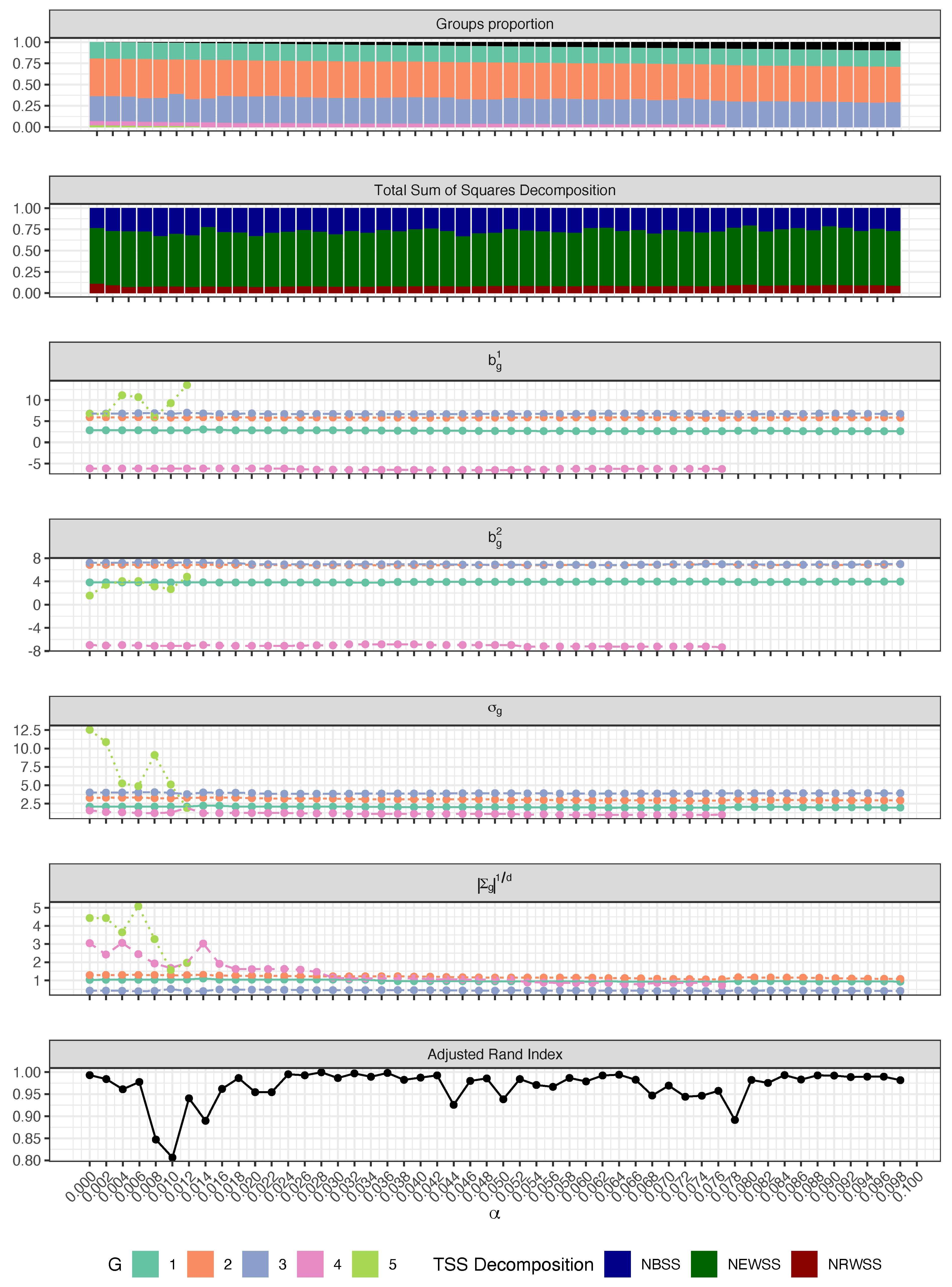
  • Groups proportion via a stacked barplot, profiling sample sizes and appearance of new clusters,
  • CWM decomposition of the total sum of squares via a stacked barplot, according to the cluster validation measure introduced in [21],
  • Regression coefficients via a G-lines plot, profiling the increase and/or decrease in parameters magnitude,
  • Regression standard deviations via a G-lines plot, profiling the increase and/or decrease in variability around the regression hyper-planes,
  • Cluster volumes via a G-lines plot, profiling the increase and/or decrease in Σ ^ g 1 / d , g = 1 , , G ,
  • ARI between consecutive cluster allocations via a line plot, following [20].
By jointly exploring the evolution in the aforementioned metrics, we are able to adequately uncover the most appropriate trimming level(s) to be employed in the subsequent analysis. Within this first monitoring step, delicate care shall be devoted to mitigating the well-known label-switching problem of mixture models. In doing so, the component-dependent metrics, estimated varying trimming levels, are directly comparable. A relabeling strategy based on the postulated model density is adopted to overcome the non-identifiability issue due to components invariance. In details, the relabeling procedure works as follows: starting from the solution obtained with the highest value of trimming, the ( 1 + d ) -dimensional quantities r g = μ ^ g , b ^ g 0 + b ^ g μ ^ g are stored for each g, g = 1 , , G . Notice that r g is nothing but the estimated marginal d-dimensional cluster mean juxtaposed to the conditional estimate according to the regression term. These quantities become the g cluster “representatives” and are used for the relabeling process of the subsequent solutions with decreasing trimming level, via the MAP rule. Whenever a solution possesses a higher number of clusters than the previous one, a new r is computed and stored as representative of this new component. Whenever a solution possesses a lower number of clusters than the previous one, the r quantity for the merged component is identified and updated in the set of representative units. Clearly, this heuristic may fail whenever the clustering structure deeply changes moving from a solution to its adjacent one. Nonetheless, when the α grid is quite dense, the failure of this procedure is itself a sign that some mechanism has spoiled the estimation process.

3.2. Step 2: Monitoring Optimal Solutions, in Terms of Validity and Stability

Having identified a/some “reasonable” value/values for α , we subsequently screen the space of solutions E 0 , obtained moving the pair of hyper-parameters c X and c y over a grid, varying the number of clusters G, conditioned on a fixed trimming level. The purpose is to obtain a reduced list O of “optimal” solutions, qualified by two features: their stability across hyper-parameter values, and their optimality in terms of (7). We elaborate on the algorithm presented in [11], to encompass the more complex framework of Cluster Weighted modeling. Given a triplet ( G , c X , c y ) , let P ( G , c X , c y ) denote the partition into G clusters, obtained by optimizing (4) under the constraints (5) and (6). Let A R I ( A , B ) denote the ARI between partitions A and B. We consider that two partitions A and B are “similar” when A R I ( A , B ) η , for a fixed threshold η . Clearly, the higher the value η the greater the number of contemplated distinct solutions. Further, let us consider the sequence G = 1 , , G M A X , where G M A X is the maximal number of clusters, and sequences c X = c 1 X , , c C X X , c y = c 1 y , , c C y y of, respectively, C X and C y possible constraint values for c X and c y . Without loss of generality and for easing the notation, in the next steps we will adopt the same grid of restrictions c = c 1 , , c C for both the covariates and the regression errors, but clearly the procedure does not require so in general. For instance, the sequence of powers of 2, c 1 = 2 0 , c 2 = 2 1 , , c C = 2 C 1 generates a sharp grid of values close to 1. In this setting, the proposed procedure for finding O , the set of T L optimal solutions is summarized in Algorithm 1, where L denotes a pre-specified upper bound for the maximum number of optimal solutions to be retained. The resulting strategy simplifies the set of operations originally proposed in [11].
Algorithm 1 Optimal solution finder
1:
Initialize the space to be explored E 0 = { ( G , c X , c y ) : G = 1 , , G M A X , c X , c y =
c 0 , , c C } and the empty list of optimal solutions O
2:
while   E t or t L do
3:
 Obtain ( G t , c X t , c y t ) = arg min ( G , c X , c y ) E t 1 T B I C ( G , c X , c y ) and append it to list O
4:
 Obtain from E t 1 the set I of triplets ( G , c X , c y ) that induce a “similar” partition to
P ( G t , c X t , c y t ) , that is
I = ( G , c X , c y ) : A R I P ( G , c X , c y ) , P ( G t , c X t , c y t ) η , for ( G , c X , c y ) E t 1
5:
E t = E t 1 I
6:
end while
7:
return O = { ( G 1 , c X 1 , c y 1 ) , , ( G T , c X T , c y T ) }
Once the optimal set has been identified, we further define two sets of “best” and “stable” intervals for each optimal solution ( G t , c X t , c y t ) in O :
B t = ( G , c X , c y ) : T B I C ( G , c X , c y ) T B I C ( G t + 1 , c X t + 1 , c y t + 1 ) and A R I P ( G t , c X t , c y t ) , P ( G , c X , c y ) η for ( G , c X , c y ) E 0 ,
S t = ( G , c X , c y ) : A R I P ( G t , c X t , c y t ) , P ( G , c X , c y ) η for ( G , c X , c y ) E 0 .
In B t , we want to identify the set of parameter values for which an optimal solution remains “best”. In doing so, we include in B t all solutions in E 0 ARI-similar to the optimal, and not worse than the next optimal solution. In S t , we want to identify the set of parameter values for which an optimal solution is "stable", including in S t all solutions ARI-similar to the optimal. It is clear that, given the definition of best and stable intervals, we implicitly require that B t S t . In the upcoming section, solutions in B t and S t will be graphically represented by darker and lighter opacity cells, with varying colors depending on which optimal solution they refer to.

4. Synthetic Experiment with Multiple Plausible Solutions

We henceforth illustrate, via a simulated scenario, how the monitoring procedures introduced in the previous section may be employed in analyzing a contaminated dataset in which no exclusive solution prevails. Consider the following data generating process (DGP)
p ( x , y ; θ ) = g = 1 4 π g ϕ ( y ; b g x + b g 0 , σ g ) ϕ 2 ( x ; μ g , Σ g ) ,
with true parameters being as follows:
π = ( 0.2 , 0.4 , 0.35 , 0.05 ) ,
μ 1 = ( 2 , 2 ) , μ 2 = ( 2 , 2 ) , μ 3 = ( 1 , 1 ) μ 4 = ( 3 , 3 )
Σ 1 = I 2 , Σ 2 = 2 0.5 0.5 1 Σ 3 = 0.5 0 0 0.5 Σ 4 = 3 0.5 0.5 2
b 1 0 = 10 , b 2 0 = 20 , b 3 0 = 20 , b 4 0 = 40
b 1 = ( 3 , 4 ) b 2 = ( 6 , 7 ) b 3 = ( 6 , 7 ) b 4 = ( 6 , 7 )
σ 1 2 = 5 , σ 2 2 = 10 , σ 3 2 = 15 , σ 4 2 = 1 .
A dataset with 980 genuine samples is generated according to (11). In addition, 20 uniformly distributed outliers are appended to the uncontaminated observations, resulting in a total of n = 1000 data units with a true contamination level equal to 0.02 . A pairs plot of the resulting 3-dimensional feature space is reported in Figure 1. It is immediately noticed that retrieving the true data partition may not be straightforward. In addition, beyond the underlying true data generating process, several solutions may be considered “reasonable” for this scenario. Given the small mixing proportion of the fourth group, one may be interested only in recovering the first three main clusters, thus preferring a solution in which the last group is entirely trimmed. Alternatively, since the conditional distributions of y given x for clusters two and three share exactly the same regression parameters, one may rationally favor a solution in which these two groups are merged together. All these options emerge when exploring the space of possible solutions E 0 = ( G , c X , c y ) : G = 1 , 5 ; c X , c y = 1 , 2 , 4 , 16 , 32 , 64 varying α { 0 , 0.02 , , 0.1 } .

4.1. Step 1: Choosing the Trimming Level
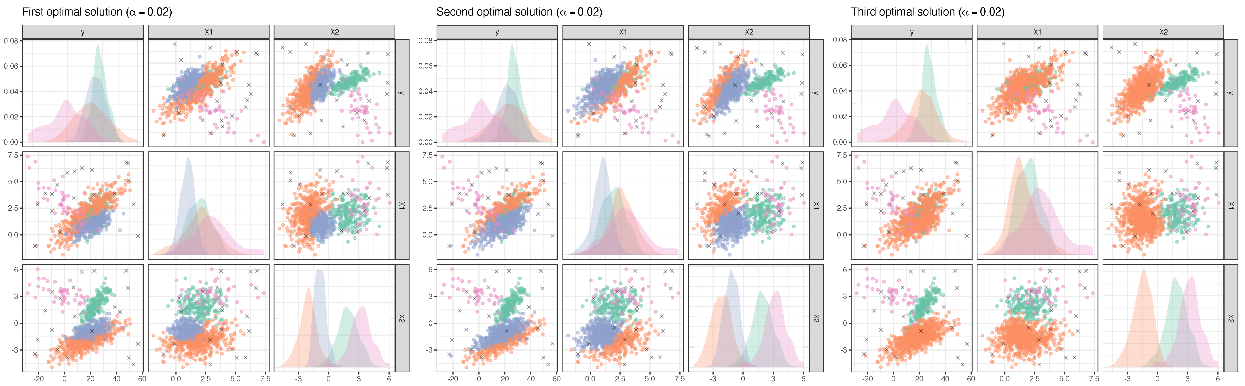
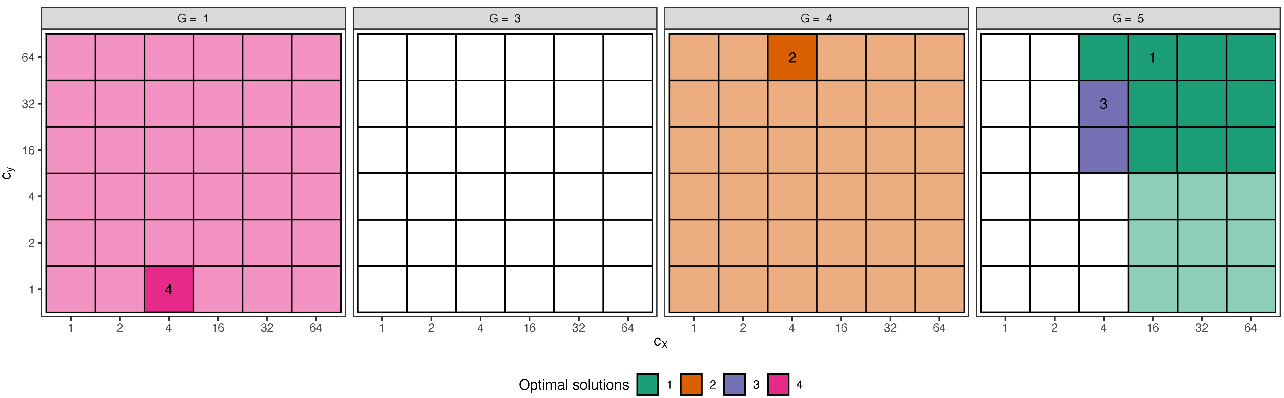
 α

The first step of the monitoring procedure results in the plots reported in Figure 2. The ARI pattern showcases two drops, respectively corresponding to the disappearance of the fifth (spurious) and the fourth group. Notwithstanding, its value never goes below 0.8 , so no unequivocal information can be achieved by monitoring this metric only. Differently, the group proportions and the line plots seem to suggest the presence of G = 4 groups. This can be appreciated by the fact that, also for the fourth cluster, the regression parameters b ^ g do not demonstrate any abrupt change, contrarily to the fifth spurious group that appears when α is set too low. Lastly, by inspecting the cluster volumes, we notice that | Σ 4 | 1 / d seems to stabilize only when the trimming level is set higher than 0.02 , that is precisely the percentage of contamination introduced in the sample. Therefore, should a practitioner be challenged to designate a trimming level using the information displayed in Figure 2, he could make two equally acceptable choices. On the one hand, setting α larger than 0.02 but smaller than 0.08 allows the CWRM to capture also the smallest cluster. On the other hand, one could be interested only in capturing the major patterns, regarding anything else as uninteresting noise: if this is the case, a trimming level greater than 0.08 shall be preferred. Ultimately, exploring untrimmed solutions, obtained by setting α = 0 , may also offer a fruitful benchmark with respect to the previous two alternatives. In all cases, the second step of the proposed procedure, described in Section 3.2, permits a thorough exploration of the resulting stability and validity of solutions within the set E 0 conditioning on the chosen α . We hereafter study the space of solutions when the trimming level is, respectively, set equal to 0.02 , 0.08 and 0.

4.2. Step 2 with α = 0.02 : Monitoring Plausible Solutions

We start by focusing on the resulting model space when α = 0.02 . In this case, the second step of the monitoring produces the plots reported in Figure 3. The T = 4 optimal solutions, obtained setting an ARI-similarity threshold η equal to 0.7 , are identified by cells with ordinal numbers whose colors with darker and lighter opacity respectively mark the sets of best and stable intervals, defined in (9) and (10). The plot in Figure 3 may be interpreted as a bi-dimensional extension, tailored for CWRM, of the car-bike plot introduced in [11]. In details, each facet encompasses models with the same number of clusters, with different values of c X (x-axis) and c y (y-axis). Likewise for the one-dimensional car-bike plot, the proposed graphical tool ensures the immediate eye-balling of the optimal solutions (cells with ordered numbers), as well as the sets of best interval and stable ones. The first optimal solution, and its best and stable intervals (darkgreen colored cells) essentially agree with the model in Equation (11), validating the fact that the true DGP is correctly recovered. The same number of estimated clusters characterizes the second optimal solution (orange colored cells), but the higher constraints enforced in the scatter matrices ( c X = 2 ) give rise to almost spherical components, where the structures of the second and third (overlapping) groups slightly differ from the true underlying ones. The third optimal solution is characterized by the fitting of G = 3 groups, with its best and stable intervals entirely covering the c X and c y grids. As anticipated at the beginning of the section, this is due to the fact that the true regression parameters for the second and third groups are exactly equal; therefore it is reasonable to contemplate a result in which these two components are entirely merged. Model results for the first three optimal solutions conditioning on α = 0.02 are represented in Figure 4. The fourth optimal model is characterized by strong restrictions in the scatter matrices and by equal regression variances, and its interpretation is less clear.

4.3. Step 2 with α = 0.08 : Monitoring Plausible Solutions

In this subsection we explore solutions conditioning on a higher trimming level, with the intention of focusing on the predominant clusters still present in the right most side of plots in Figure 2. The resulting T = 4 optimal solutions are reported in Figure 5. As expected, the first identified optimal model possesses G = 3 clusters, for which the fourth group, with the smallest mixing proportion, entirely falls within the set of trimmed units. Interestingly, the second and third optimal solutions suggest the presence of G = 4 clusters: by inspecting the induced data partition in Figure 6 we notice that the original fourth component is still partially recovered when α = 0.08 . Even though the stability of the solution is much lower due to the higher trimming level, comparing these results with those outlined in the previous subsection indicates that the fourth group, albeit small, shall probably be included in the fitting process. Lastly, we observe that models in which components two and three are merged together define a plausible clustering partition again, as highlighted by the fourth optimal solution and its associated stable interval.

4.4. Step 2 with α = 0 : Monitoring Plausible Solutions

The monitoring procedure for models with no trimming enforced in the ML estimation is graphically summarized in Figure 7. The first optimal solution efficiently well recovers the true DGP, in which an extra component with high variance, in both the regressions and the scatter matrices, is nevertheless needed to model the background noise. Similar to what was experienced for the previous choices of α , the option of merging components two and three defines the second optimal solution, spanning the entire grid of c X and c y for G = 4 (see Figure 8). However, the most unexpected behavior appears when looking at the fourth optimal model: the groups heterogeneity is entirely lost and a single regression term is deemed sufficient to explain the entire dataset. This shall be interpreted as a wake-up call that a noise mechanism is by some means masking the clustering structure. Notice that contamination of only 2 % is sufficient to induce such unwanted behavior. Clearly, by exploring Figure 2 in the first step it should immediately be apparent that a small percentage of trimming is necessary to ensure stability in the estimation. The α = 0 case has been examined to cast light on the harmful effect noise produces when contamination is not properly taken care of, further justifying the applicability of our two-steps monitoring procedure.
The described analyses have been carried out by means of the R programming language: software routines, including the method implementation and the scripts necessary to reproduce the results presented in this section are openly available at https://github.com/AndreaCappozzo/STATS-monitoring_CWRM (accessed on 18 June 2021). Regarding the computational cost it is clear that, by its very nature, the proposed method is computationally expensive since many parameters combinations have to be estimated. Nevertheless, the overall computational load can be alleviated by either using parallelization or optimal solutions as reasonable initializations for contiguous problems.

5. Concluding Remarks

The present paper has focused on the problem of identifying a set of sensible hyper-parameters in the framework of robust mixtures of regressions with random covariates. By relying on the logic that no unique solution exists when it comes to perform cluster analysis, we have proposed a two-steps monitoring procedure for helping practitioners choose the best model, according to their judgment, within a reduced set of optimal solutions. To this extent, we have introduced a dedicated criterion for performing model selection, based on a penalty that depends on the doubly-constrained maximization problem. In exploring the space of solutions, we have first selected a plausible trimming level(s) by means of specific representations tailored for the CWRM framework. Secondly, conditioning on one or more α values determined in the first step, we have defined a semi-automatic procedure for screening the model hyper-parameters, ranking subsets of solutions that are ARI-similar and arranged by the penalized criterion. The thorough analysis of a challenging synthetic experiment has demonstrated the applicability of our proposal.
Our method has commonalities with another novel monitoring methodology for semiautomatic robust regression clustering [22]: they both appeared almost concomitantly in the literature. The cited work is certainly related to the one we have proposed, thus a short remark is in order to highlight the respective commonalities and distinctive features of the two proposals. First off, the main focus of [22] is on the classical mixture of robust regressions, without taking into account distribution on the covariates. Certainly the method proposed in [22] is quite general: the authors themselves suggest that it is sufficient to fix c X to a large number, e.g., c X = 128 , to adapt their procedure to work for CWRM. We however would like to stress that our methodology is specifically designed to deal with situations in which the covariates are random, so much so that we explicitly account for different values of c X in our monitoring step. Secondly, how the model space is explored differs in the two proposals: in our first step we let the best model be selected conditioning on the trimming level, whereas in [22] the authors firstly identify the best G and c y and then, conditioning on these two values, they monitor α . Lastly, the label switching problem is differently handled: while we suggest a density-based metric to designate cluster representatives, in [22] the relabeling strategy is based on other criteria such as the estimated regression coefficients varying trimming level. Overall then, both contributions possess distinctive peculiarities, suggesting de facto two different approaches for solving a similar, and, as it seems, very relevant, problem.
Further research directions include the employment of the devised methodological procedure in a wide set of applications, further validating its relevance in real-world contexts. Additionally, as suggested by an anonymous reviewer, the present work may foster the development of a broader set of graphical tools useful for checking the sensitivity of the CWRM to miss-specifications of ϕ d . That is, the group-wise Gaussian assumption may not always hold for the set of covariates, and it would be interesting to monitor at which extent deviations from Gaussianity can impact the hyper-parameters specification. These topics will be the object of future research.

Author Contributions

Conceptualization, F.G., A.C., L.A.G.E. and A.M.-I.; methodology, F.G., A.C., L.A.G.E. and A.M.-I.; software, A.C.; validation, F.G., A.C., L.A.G.E. and A.M.-I.; writing—original draft preparation, F.G. and A.C.; writing—review and editing, L.A.G.E. and A.M.-I.; visualization, A.C. All authors have read and agreed to the published version of the manuscript.

Funding

This research was funded by Milano-Bicocca University Fund for Scientific Research, 2019-ATE-0076. Andrea Cappozzo’s work is supported by the Research Programme: “Integration between study design and data analytics for generating credible evidence in the field of healthcare from heterogeneous sources of structured and unstructured data”. Luis A. García-Escudero and Agustín Mayo Iscar work is supported by Spanish Ministerio de Economía y Competitividad, grant MTM2017-86061-C2-1-P, and by Consejería de Educación de la Junta de Castilla y León and FEDER, grant VA005P17 and VA002G18.

Institutional Review Board Statement

Not applicable.

Informed Consent Statement

Not applicable.

Data Availability Statement

The simulated data presented in this study are openly available at https://github.com/AndreaCappozzo/STATS-monitoring_CWRM.

Acknowledgments

The authors wish to thank four anonymous referees and the Associate Editor for their helpful comments.

Conflicts of Interest

The authors declare no conflict of interest.

References

  1. Everitt, B.S.; Landau, S.; Leese, M.; Stahl, D. Cluster Analysis; Wiley Series in Probability and Statistics; John Wiley & Sons, Ltd.: Chichester, UK, 2011; Volume 100, pp. 603–616. [Google Scholar] [CrossRef]
  2. McLachlan, J.; Peel, D. Finite Mixture Models; John Wiley & Sons, Inc.: Hoboken, NJ, USA, 2000. [Google Scholar]
  3. Bouveyron, C.; Celeux, G.; Murphy, T.B.; Raftery, A.E. Model-Based Clustering and Classification for Data Science; Cambridge University Press: Cambridge, UK, 2019; Volume 50. [Google Scholar] [CrossRef]
  4. Hennig, C. What are the true clusters? Pattern Recognit. Lett. 2015, 64, 53–62. [Google Scholar] [CrossRef] [Green Version]
  5. Von Luxburg, U.; Ben-David, S.; Luxburg, U.V. Towards a statistical theory of clustering. In Proceedings of the Pascal Workshop on Statistics and Optimization of Clustering, London, UK, 4–5 July 2005; pp. 20–26. [Google Scholar]
  6. Ackerman, M.; Ben-David, S. Measures of clustering quality: Aworking set of axioms for clustering. In Proceedings of the 21st International Conference on Neural Information Processing Systems, Vancouver, BC, Canada, 8–10 December 2008; pp. 121–128. [Google Scholar]
  7. Milligan, G.W.; Cooper, M.C. An examination of procedures for determining the number of clusters in a data set. Psychometrika 1985, 50, 159–179. [Google Scholar] [CrossRef]
  8. Rousseeuw, P.J. Silhouettes: A graphical aid to the interpretation and validation of cluster analysis. J. Comput. Appl. Math. 1987, 20, 53–65. [Google Scholar] [CrossRef] [Green Version]
  9. Tibshirani, R.; Walther, G.; Hastie, T. Estimating the number of clusters in a data set via the gap statistic. J. R. Stat. Soc. Ser. B (Stat. Methodol.) 2001, 63, 411–423. [Google Scholar] [CrossRef]
  10. Cerioli, A.; Riani, M.; Atkinson, A.C.; Corbellini, A. The power of monitoring: How to make the most of a contaminated multivariate sample. Stat. Methods Appl. 2018, 27, 661–666. [Google Scholar] [CrossRef]
  11. Cerioli, A.; García-Escudero, L.A.; Mayo-Iscar, A.; Riani, M. Finding the number of normal groups in model-based clustering via constrained likelihoods. J. Comput. Graph. Stat. 2018, 27, 404–416. [Google Scholar] [CrossRef] [Green Version]
  12. Gershenfeld, N. Nonlinear Inference and Cluster-Weighted Modeling. Ann. N. Y. Acad. Sci. 1997, 808, 18–24. [Google Scholar] [CrossRef]
  13. Huber, P.J.; Ronchetti, E.M. Robust Statistics; Wiley Series in Probability and Statistics; John Wiley & Sons, Inc.: Hoboken, NJ, USA, 2009. [Google Scholar] [CrossRef]
  14. García-Escudero, L.A.; Gordaliza, A.; Greselin, F.; Ingrassia, S.; Mayo-Iscar, A. Robust estimation of mixtures of regressions with random covariates, via trimming and constraints. Stat. Comput. 2017, 27, 377–402. [Google Scholar] [CrossRef] [Green Version]
  15. Neykov, N.; Filzmoser, P.; Dimova, R.; Neytchev, P. Robust fitting of mixtures using the trimmed likelihood estimator. Comput. Stat. Data Anal. 2007, 52, 299–308. [Google Scholar] [CrossRef]
  16. Hathaway, R.J. A Constrained Formulation of Maximum-Likelihood Estimation for Normal Mixture Distributions. Ann. Stat. 1985, 13, 795–800. [Google Scholar] [CrossRef]
  17. Torti, F.; Perrotta, D.; Riani, M.; Cerioli, A. Assessing trimming methodologies for clustering linear regression data. Adv. Data Anal. Classif. 2019, 13, 227–257. [Google Scholar] [CrossRef] [Green Version]
  18. Claeskens, G.; Hjort, N.L. Model Selection and Model Averaging; Cambridge University Press: Cambridge, UK, 2008. [Google Scholar] [CrossRef]
  19. Schwarz, G. Estimating the dimension of a model. Ann. Stat. 1978, 6, 461–464. [Google Scholar] [CrossRef]
  20. Riani, M.; Atkinson, A.C.; Cerioli, A.; Corbellini, A. Efficient robust methods via monitoring for clustering and multivariate data analysis. Pattern Recognit. 2019, 88, 246–260. [Google Scholar] [CrossRef] [Green Version]
  21. Ingrassia, S.; Punzo, A. Cluster Validation for Mixtures of Regressions via the Total Sum of Squares Decomposition. J. Classif. 2020, 37, 526–547. [Google Scholar] [CrossRef]
  22. Torti, F.; Riani, M.; Morelli, G. Semiautomatic robust regression clustering of international trade data. Stat. Methods Appl. 2021. [Google Scholar] [CrossRef] [PubMed]
Figure 1. Pairs plot of the synthetic dataset generated according to (11), and resulting true underlying partition.
Stats 04 00036 g001
Figure 2. Step 1: Groups proportion (black bars denote the trimmed units), total sum of squares decomposition, regression coefficients, standard deviations, cluster volumes and ARI between consecutive cluster allocations as a function of the trimming proportion α .
Stats 04 00036 g002
Figure 3. Step 2: monitoring the optimal solutions (cells with ordered numbers), best interval solutions (darker opacity cells) and stable solutions (lighter opacity cells), varying G, c X (x-axis) and c y (y-axis) in E 0 . Trimming level α = 0.02 .
Stats 04 00036 g003
Figure 4. Pairs plots for the first, second and third optimal solution resulting from the second step of the monitoring procedure. Trimmed units are denoted by ×. Trimming level α = 0.02 .
Stats 04 00036 g004
Figure 5. Step 2: monitoring the optimal solutions (cells with ordered numbers), best interval solutions (darker opacity cells) and stable solutions (lighter opacity cells), varying G, c X (x-axis) and c y (y-axis) in E 0 . Trimming level α = 0.08 .
Stats 04 00036 g005
Figure 6. Pairs plots for the first, second and third optimal solution resulting from the second step of the monitoring procedure. Trimmed units are denoted by ×. Trimming level α = 0.08 .
Stats 04 00036 g006
Figure 7. Step 2: monitoring the optimal solutions (cells with ordered numbers), best interval solutions (darker opacity cells) and stable solutions (lighter opacity cells), varying G, c X (x-axis) and c y (y-axis) in E 0 . Trimming level α = 0 .
Stats 04 00036 g007
Figure 8. Pairs plots for the first, second and third optimal solution resulting from the second step of the monitoring procedure. Trimming level α = 0 .
Stats 04 00036 g008
Publisher’s Note: MDPI stays neutral with regard to jurisdictional claims in published maps and institutional affiliations.

