A Constrained Generalized Functional Linear Model for Multi-Loci Genetic Mapping

Abstract

In genome-wide association studies (GWAS), efficient incorporation of linkage disequilibria (LD) among densely typed genetic variants into association analysis is a critical yet challenging problem. Functional linear models (FLM), which impose a smoothing structure on the coefficients of correlated covariates, are advantageous in genetic mapping of multiple variants with high LD. Here we propose a novel constrained generalized FLM (cGFLM) framework to perform simultaneous association tests on a block of linked SNPs with various trait types, including continuous, binary and zero-inflated count phenotypes. The new cGFLM applies a set of inequality constraints on the FLM to ensure model identifiability under different genetic codings. The method is implemented via B-splines, and an augmented Lagrangian algorithm is employed for parameter estimation. For hypotheses testing, a test statistic that accounts for the model constraints was derived, following a mixture of chi-square distributions. Simulation results show that cGFLM is effective in identifying causal loci and gene clusters compared to several competing methods based on single markers and SKAT-C. We applied the proposed method to analyze a candidate gene-based COGEND study and a large-scale GWAS data on dental caries risk.

1. Introduction

Recent advances in technology have facilitated the development of association studies using a highly dense map of genetic markers, such as single nucleotide polymorphisms (SNPs). Nowadays, up to a million SNPs can be readily genotyped along the human genome for thousands of subjects. Even though analyses based on univariate tests are still popular and useful as pre-screening techniques [1], such methods have a major drawback—the high correlation and composite effect among multiple genetic variants are omitted. To accommodate this challenge, a few more advanced statistical methods that are based on multiple linked SNPs have been developed in recent years [2,3,4,5], aiming to improve the power of associations between genetic markers and phenotypic traits of interest.

As SNPs naturally cluster together and form the so-called linkage disequilibrium (LD) blocks, multi-loci association tests that take into account this special genomic structure are usually more powerful than single SNP-based ones [2,3,4,5]. Further, due to this locally connected/correlated LD structure, if a casual SNP, even unobserved in some cases, exists in one LD block, its information, i.e., genetic effect, can be partially carried and jointly represented by its neighboring SNPs in the same block, which increases the likelihood of the causal SNPs being detected. Another benefit of testing at the LD block level is on multiple test adjustment in GWAS, including not only significant reduction of the total number of tests, but also improvement on the independence of the tests. Several multi-SNP methods have been proposed, such as principal component analysis [2,6], entropy-based methods [7,8], kernel machine methods (SKAT, SKAT-C and CKAT) [3,5] and two-marker LD mapping [4]. In addition, some variable selection models, such as LASSO [9,10] and smoothed minimax concave penalized regression (SMCP) [11], were applied to identify a core subset of potential causal variants. Although these methods are useful, most of them overlook marker ordering information in their physical positions.

Functional linear models (FLMs) serve as a good solution to the above-mentioned problems, as it can effectively preserve the intrinsic correlation structure and spatial information of SNPs in an LD [12]. In essence, FLMs take into account the effect that neighboring correlated SNPs in an LD would show similar genetic effects, and treat the regression coefficients of these SNPs with an explicit functional form. The smooth coefficient function can be further expanded in terms of spline bases, which allows for substantial dimension reduction in parameter estimation [12,13]. Both functional principal component analysis (FPCA) and beta-smooth only approaches have been applied to construct the FLMs [12,14,15,16]. Since the beta-smooth only approach is more straightforward, it was used for the construction of FLM in this study.

One critical issue with FLM is that the fitted coefficient functions are often noisy and hard to interpret. They usually fluctuate dramatically due to several reasons: (1) Strong LD among nearby SNPs causes multicollinearity, which leads to erratic changes in the signs of adjacent functional coefficients; (2) FLMs cannot yield estimates that are exactly zero over regions with no significant association, thus generating unnatural wiggles in the fitted genetic function; (3) population-specific phenomena such as mutation, genetic drift, population structure and variations in allele frequencies result in the LD not decaying with distance. Excessive local fluctuation may be relieved by adding a smoothness penalty in the model or controlling the number of spline bases. However, these methods are still not able to identify the null regions in which the coefficient function should be zero and may suffer from loss of detection power due to oversmoothing. In addition, no proper test other than the permutation approach is available for penalty-based methods, which brings heavy computational burden to large-scale studies.

In this paper, we propose a novel constrained generalized functional linear model (cGFLM) for flexible and reasonable multi-loci genetic mapping on a block of correlated genetic variants. The cGFLM retains the merits of FLM such as preserving the spatial and LD information among genetic markers, as well as compressing the high-dimensional problem into aggregate inference about several smoothing components. In addition to these benefits, the cGFLM is more powerful and enables easier interpretation of the functional coefficients. Specifically, we reconstruct FLM by separating the genetic effect into two sign-specific coefficient functions and imposing an equality constraint to encourage overall spatial sparsity. The cGFLM tends to constrain the functional coefficients to be zero in “null regions” where no determinative positive or negative effect is present.

We further extend the cGFLM framework to several types of quantitative traits, such as continuous, binary and count data. We put more focus on count traits as they are common in practice but relatively less mentioned in the literature. Poisson and negative binomial (NB) models provide tractable methods to most count traits, however, in traits with excessive zeros, zero-inflated Poisson (ZIP) or negative binomial (ZINB) models were also developed [17]. Since the ZINB is the most complicated model here, we discuss how to apply the cGFLM to it in more detail. Applications of cGFLM to other models would be similar.

The remainder of the article is organized as follows. In Section 2 and Section 3, we introduce a generalized functional linear model (GFLM) framework, discussing the continuous and categorical traits (Section 2) and then zero-inflated negative binomial phenotypic traits (Section 3). In Section 4, we describe the proposed cGFLM and cGFLM-ZINB models, as well as their estimation and testing processes. In Section 5, we present Monte Carlo simulations to validate the proposed test and compare our model with several alternative methods. In Section 6 and Section 7, we apply the proposed method to the COGEND (The Collaborative Genetic Study of Nicotine Dependence) and Dental Caries GWAS data. Section 8 and Section 9 are the discussion and conclusion, respectively.

2. Generalized Functional Linear Model

Suppose n subjects are sampled, each characterized by p linked SNP markers $j=1,\dots ,p$, where $m_j$ is the spatial location of SNP marker j with $0\le m_1<\cdots <m_p$. SNP location can be measured by the distance of a SNP from starting position of a block. Denote the SNP genotype at marker position $m_j$ for subject i as $X_i\left(m_j\right)$. Suppose the genotypes of a SNP are AA, Aa and aa, which are coded as 0, 1 and 2, according to the number of copies of the allele a. That is,

$$X_i\left(m_j\right)=\left\{\begin{array}{cc}0,\hfill & \mathrm{if}\mathrm{the}\mathrm{genotype}\mathrm{of}\mathrm{SNP}j\mathrm{at}\mathrm{position}{m}_j\mathrm{is}AA;\hfill \\ 1,\hfill & \mathrm{if}\mathrm{the}\mathrm{genotype}\mathrm{of}\mathrm{SNP}j\mathrm{at}\mathrm{position}{m}_j\mathrm{is}Aa;\hfill \\ 2,\hfill & \mathrm{if}\mathrm{the}\mathrm{genotype}\mathrm{of}\mathrm{SNP}j\mathrm{at}\mathrm{position}{m}_j\mathrm{is}aa.\hfill \end{array}\right.$$

(1)

Suppose the genetic effect is denoted by $\beta \left(m\right)$, a smooth coefficient function over all marker positions m in an LD block. The value of the smooth coefficient function at marker position $m_j$ is then $\beta \left(m_j\right)$. Further, suppose a set of other covariates ${\mathit{z}}_{\mathit{i}}={(z_{i1},\dots ,z_{iq})}^{\top }$ are also observed for subject i and let $\mathit{\alpha }={({\alpha }_1,\dots ,{\alpha }_q)}^{\top }$ be the $q\times 1$ vector of their corresponding coefficients. The global-featured effect is included as the intercept, denoted as ${\alpha }_0$. For the ith subject, let $y_i$ denote its phenotypic response. If $y_i$s are continuous, a functional linear model (FLM) can be formulated as

$$y_i={\alpha }_0+\sum _{u=1}^q{z}_{iu}{\alpha }_u+\sum _{j=1}^p{X}_i\left(m_j\right)\beta \left(m_j\right)+{ϵ}_i,{ϵ}_i\sim N(0,{\sigma }_{ϵ}^2).$$

(2)

This type of association has been explored in [12,14]. Alternatively, if $y_i$s are categorical, a link function $g(·)$ can be applied to to transform its mean $\mu \left(y_i\right)=E\left(y_i\right)$ to be $g\left(\mu \left(y_i\right)\right)$. In this case, a generalized functional linear model (GFLM) can be formulated as

$$g\left(\mu \left(y_i\right)\right)={\alpha }_0+\sum _{u=1}^q{z}_{iu}{\alpha }_u+\sum _{j=1}^p{X}_i\left(m_j\right)\beta \left(m_j\right).$$

(3)

In the FLM/GFLM above, the genetic effects of a block of SNPs are assumed to be a smooth function. In other words, SNPs located close to each other are expected to show similar effects.

Here we represent $\beta \left(m\right)$ with B-splines and express $\beta \left(m\right)$ as

$$\beta \left(m\right)=\sum _{r=1}^d{\gamma }_r{B}_r\left(m\right)=\mathit{B}\left(m\right)\mathit{\gamma },$$

(4)

where $d\ge 1$ is the number of basis functions, ${\mathit{\gamma }}_{d\times 1}={({\gamma }_1,\dots ,{\gamma }_d)}^{\top }$ is a vector of real-valued coefficients, $(B_1,\dots ,B_d)$ is a set of d basis functions, and $\mathit{B}\left(m\right)=(B_1\left(m\right),\dots ,B_d\left(m\right))$ is a vector for the d basis functions evaluated at position m. Let ${\mathit{y}}_{n\times 1}={(y_1,\dots ,y_n)}^{\top },{\mathit{Z}}_{n\times q}={({\mathit{z}}_{\mathit{1}},\dots ,{\mathit{z}}_{\mathit{n}})}^{\top }$,

$${\mathit{X}}_{n\times p}=\left(\begin{array}{ccc}{X}_1\left(m_1\right)& \cdots & X_1\left(m_p\right)\\ ⋮& ⋮& ⋮\\ X_n\left(m_1\right)& \cdots & X_n\left(m_p\right)\end{array}\right)\mathrm{and}{\mathit{B}}_{p\times d}=\left(\begin{array}{ccc}{B}_1\left(m_1\right)& \cdots & B_d\left(m_1\right)\\ ⋮& ⋮& ⋮\\ B_1\left(m_p\right)& \cdots & B_d\left(m_p\right)\end{array}\right).$$

(5)

In matrix form, the GFLM in (3) can be reformulated as

$$\begin{array}{cc}\hfill g\left(\mu \right(\mathit{y}\left)\right)& ={\alpha }_0+\mathit{Z}\mathit{\alpha }+\mathit{X}\mathit{\beta }\hfill \\ \hfill & ={\alpha }_0+\mathit{Z}\mathit{\alpha }+\mathit{XB}\mathit{\gamma }\hfill \\ \hfill & =\left(\begin{array}{ccc}\mathbf{1}& \mathit{Z}& \mathit{XB}\end{array}\right){\left(\begin{array}{ccc}{\alpha }_0& \mathit{\alpha }& \mathit{\gamma }\end{array}\right)}^{\top }.\hfill \end{array}$$

(6)

Suppose the responses ${\mathit{y}}_{n\times 1}$ are i.i.d. samples from a distribution with density $f(y;\mathit{\beta })$. By substituting $\mathit{\beta }$ with $\mathit{B}\gamma$, the number of parameters changes from $(p+q+1)$ to $(d+q+1)$. Then the log-likelihood function can be expressed as

$$l({\alpha }_0,\mathit{\alpha },\mathit{\gamma })=\sum _{i=1}^{n}logf(y_i;{\alpha }_0,\mathit{\alpha },\mathit{\gamma })$$

(7)

The maximum likelihood estimators (MLE) for parameters can be computed by maximizing the log-likelihood function

$$({\widehat{\alpha }}_0,\widehat{\mathit{\alpha }},\widehat{\mathit{\gamma }})=arg\underset{{\alpha }_0,\mathit{\alpha },\mathit{\gamma }}{max}l({\alpha }_0,\mathit{\alpha },\mathit{\gamma }).$$

(8)

Since we are modeling a block of SNPs simultaneously in (3), the hypothesis test of association between genetic variants and phenotypic trait will be made at the block level. That is,

$$\begin{array}{cc}{\mathrm{H}}_0:\hfill & \beta \left(m_j\right)=0,\mathrm{for}\mathrm{all}j=1,\dots ,p.\hfill \\ {\mathrm{H}}_a:\hfill & \mathrm{Not}{\mathrm{H}}_0.\hfill \end{array}$$

(9)

Approximately, the hypotheses can also be expressed as:

$$\begin{array}{cc}{\mathrm{H}}_0:\hfill & {\gamma }_r=0,\mathrm{for}\mathrm{all}r=1,\dots ,d.\hfill \\ {\mathrm{H}}_a:\hfill & {\gamma }_r\in {\mathbb{R}}^d.\hfill \end{array}$$

(10)

The likelihood ratio test (LRT) can be applied to draw inference about whether a block of SNPs may be associated with the phenotypic trait. Under ${\mathrm{H}}_0$, the LRT statistic, defined as $-2(l_0-l_1)$, follows asymptotically a ${\chi }_d^2$ distribution (Chi-square distribution with df = d, the number of basis vectors used in Equation (5)).

3. GFLM for Zero-Inflated Negative Binomial (ZINB) Traits

Most count traits can be modeled with Poisson or negative binomial (NB) distributions. However, when excessive zeroes are present in the data, a zero-inflated Poisson or negative binomial regression framework needs to be employed [17], which utilizes a latent Bernoulli distribution and a Poisson distribution to incorporate explanatory variables. In this section, we describe a GFLM framework for count traits that follow a ZINB distribution.

To illustrate the ZINB model, we use dental caries, more commonly known as tooth decay, as an example. Let Y denote the number of dental caries, and the probability distribution of Y is given as:

$$\begin{array}{c}L\sim \mathrm{Bernoulli}\left(\pi \right);\\ Pr(Y=0|L=1)=1;\\ Pr(Y=k|L=0)\sim NB(\mu ,\varphi ),k=0,1,\dots \end{array}$$

(11)

Here L is a latent Bernoulli random variable that categorizes caries “risk” into two states: “risk-free” (L = 1) and “risky” (L = 0). $\pi$ is the probability of $L=1$, $\mu$ and $\varphi$ are the mean and dispersion parameter of the NB distribution, respectively.

In a ZINB regression model, let $y_i$ denote the observation of number of caries for subject $i,i=1,\dots ,n$. Then,

$$y_i\sim \left\{\begin{array}{cc}0,\hfill & \mathrm{with}\mathrm{probability}{\pi }_i;\hfill \\ NB({\mu }_i,\lambda ),\hfill & \mathrm{with}\mathrm{probability}1-{\pi }_i.\hfill \end{array}\right.$$

(12)

We can see that zeroes may come from two sources: the conditional point mass distribution or the conditional NB distribution. Thus, the occurrence of dental caries $y_i$ is:

$$y_i=\left\{\begin{array}{cc}0,\hfill & \mathrm{with}\mathrm{probability}{\pi }_i+(1-{\pi }_i){\left(\frac{\varphi }{\varphi +{\mu }_i}\right)}^{\varphi };\hfill \\ k,\hfill & \mathrm{with}\mathrm{probability}(1-{\pi }_i)\frac{\mathsf{\Gamma }(\varphi +k)}{k!\mathsf{\Gamma }\left(\varphi \right)}{\left(\frac{\varphi }{\varphi +{\mu }_i}\right)}^{\varphi }{\left(\frac{{\mu }_i}{\varphi +{\mu }_i}\right)}^k,\mathrm{k}=1,2,\dots \hfill \end{array}\right.$$

(13)

An expectation-maximization (EM) algorithm can be applied to estimate the parameters in the ZINB model. Suppose at step t, the parameter estimates are $({\pi }^{\left(t\right)},{\mu }^{\left(t\right)},{\varphi }^t)$. Then the detailed EM implementation is given as follows.

E-step

For subject $i,i=1,\dots ,n$, estimate $L_i$ by its conditional mean

$$L_i^{\left(t\right)}=E_{L|y_i,{\pi }^{\left(t\right)},{\mu }^{\left(t\right)},{\varphi }^{\left(t\right)}}\left(L_i\right)=\left\{\begin{array}{cc}0,\hfill & y_i>0;\hfill \\ \frac{{\pi }^{\left(t\right)}}{{\pi }^{\left(t\right)}+(1-{\pi }^{\left(t\right)}){\left(\frac{{\varphi }^t}{{\varphi }^{\left(t\right)}+{\mu }^{\left(t\right)}}\right)}^{{\varphi }^{\left(t\right)}}},\hfill & y_i=0.\hfill \end{array}\right.$$

(14)

M-step

• Find ${\pi }^{(t+1)}$ by maximizing

  $$l_{Ber}\left(\pi \right|\mathit{y},{\mathit{z}}^{\left(t\right)})=\sum _{i=1}^n{L}_i^{\left(t\right)}\log \left(\pi \right)+(1-L_i^{\left(t\right)})\log (1-\pi )$$

  (15)
• Find ${\mu }^{(t+1)},{\varphi }^{(t+1)}i$ by maximizing

  $$l_{NB}(\mu ,\varphi |\mathit{y},{\mathit{z}}^{\left(t\right)})=\sum _{i=1}^n(1-L_i^{\left(t\right)})\log \frac{\mathsf{\Gamma }(\varphi +y_i)}{y_i!\mathsf{\Gamma }\left(\varphi \right)}{\left(\frac{\varphi }{\varphi +\mu }\right)}^{\varphi }{\left(\frac{\mu }{\varphi +\mu }\right)}^{y_i}$$

  (16)

The maximization can be performed by the Newton–Raphson algorithm for the two models int the M-step simultaneously.

Using the same notations as in the previous section, the Bernoulli probabilities and the negative binomial means can be transformed using the logit and the log links, respectively, and are modeled as follows:

$$\mathrm{logit}\left({\pi }_i\right)=\log \left(\frac{{\pi }_i}{1-{\pi }_i}\right)={\alpha }_0^{Ber}+\sum _{u=1}^q{z}_{iu}{\alpha }_u^{Ber}+\sum _{j=1}^p{X}_i\left(m_j\right){\beta }^{Ber}\left(m_j\right),$$

(17)

and

$$\log \left({\mu }_i\right)={\alpha }_0^{NB}+\sum _{u=1}^q{z}_{iu}{\alpha }_u^{NB}+\sum _{j=1}^p{X}_i\left(m_j\right){\beta }^{NB}\left(m_j\right).$$

(18)

Since usually we do not have strong pre-assumption about genetic components and covariates, the same sets of genetic components and covariates can be used in both Bernoulli and NB models simultaneously. For univariate analyses on single SNPs, it is equivalent to the case that one LD block only contains one SNP, and we can simply set $p=1$ in the above equations. For multi-loci mapping purposes, we set all SNPs in an LD block as input/explanatory variables.

We substitute the unstructured coefficients to functional coefficients, which are represented by linear combination of B-Splines. That is, Equation (5) is plugged into the coefficients for both the latent Bernoulli model and NB model to form the GFLM-ZINB model. Using the same notation above, the GFLM-ZINB model is reformulated as:

$$\begin{array}{c}\hfill \mathrm{logit}\left({\pi }_i\right)=\left(\begin{array}{ccc}1& {\mathit{Z}}_i& {\mathit{X}}_{\mathit{i}}{\mathit{B}}^{\left(\mathit{Ber}\right)}\end{array}\right){\left(\begin{array}{ccc}{\alpha }_0^{Ber}& {\mathit{\alpha }}^{Ber}& {\mathit{\gamma }}_{{\mathit{d}}_{\mathit{B}\mathit{e}\mathit{r}}\times \mathbf{1}}^{Ber}\end{array}\right)}^{\top }=U_i^{Ber}{\eta }^{Ber}.\end{array}$$

(19)

$$\begin{array}{cc}\hfill \log \left({\mu }_i\right)& =\left(\begin{array}{ccc}1& {\mathit{Z}}_i& {\mathit{X}}_{\mathit{i}}{\mathit{B}}^{\left(\mathit{NB}\right)}\end{array}\right){\left(\begin{array}{ccc}{\alpha }_0^{NB}& {\mathit{\alpha }}^{NB}& {\mathit{\gamma }}_{{\mathit{d}}_{\mathit{B}\mathit{e}\mathit{r}}\times \mathbf{1}}^{Ber}\end{array}\right)}^{\top }=U_i^{NB}{\eta }^{NB}.\hfill \end{array}$$

Then we can estimate the parameters using an EM Algorithm again, which is implemented as follows.

• Let ${\widehat{L}}_i^{\left(t\right)}=\frac{{\pi }_i^{\left(t\right)}}{{\pi }_i^{\left(t\right)}+(1-{\pi }_i^{\left(t\right)}){\left(\frac{{\varphi }^t}{{\varphi }^{\left(t\right)}+{\mu }_i^{\left(t\right)}}\right)}^{{\varphi }^{\left(t\right)}}}\mathbb{I}(y_i=0)$
• • Perform logistic regression of ${\widehat{L}}_i^{\left(t\right)}$ on $U^{Ber}$ to estimate ${\eta }^{{Ber}^{(t+1)}}$.
  • Perform weighted negative binomial regression of y on $U^{NB}$ with weights $1-{\widehat{L}}_i^{\left(t\right)}$ to obtain estimate ${\eta }^{{NB}^{(t+1)}}$ and ${\varphi }^{(t+1)}$.
• Let ${\pi }_i^{(t+1)}=\frac{exp\left(U_i^{Ber}{\eta }^{{Ber}^{(t+1)}}\right)}{1+exp\left(U_i^{Ber}{\eta }^{{Ber}^{(t+1)}}\right)}$ and ${\mu }^{(t+1)}=exp\left(U_i^{NB}{\eta }^{{NB}^{(t+1)}}\right)$, iterate back to step 1.

For hypothesis testing, since we model a block of SNPs simultaneously, the test of association between genetic variants and a phenotypic trait will be made at the block level. In the meantime, we have two sets of parameters, one for the latent Bernoulli model and one for the negative binomial model. The hypothesis test should consider the overall effect of both models. That is, we consider testing at least one coefficients from either model being nonzero. Note that we obtained dimension reduction by changing the estimator of interest from the $2p$-dimensional ${\beta }^{Ber}\left(m_j\right)$ and ${\beta }^{NB}\left(m_j\right),j=1,\dots ,p$ to the $(d_{Ber}+d_{NB})$-dimensional ${\mathit{\gamma }}_{d_{Ber}\times 1}^{Ber}$ and ${\mathit{\gamma }}_{d_{NB}\times 1}^{NB}$ by applying the functional coefficients implemented via the B-spline bases. The hypotheses are formulated as

$$\begin{array}{cc}{\mathrm{H}}_0:\hfill & {\mathit{\gamma }}_b^{Ber}=0,{\mathit{\gamma }}_m^{NB}=0,\mathrm{for}\mathrm{all}b,n.\hfill \\ {\mathrm{H}}_a:\hfill & \mathrm{Not}{\mathrm{H}}_0.\hfill \end{array}$$

(20)

The likelihood ratio test (LRT) can be applied to draw inference about whether a block of SNPs may be associated with the phenotypic trait. Under ${\mathrm{H}}_0$, the LRT statistic asymptotically follows a ${\chi }_{d_{Ber}+d_{NB}}^2$ distribution (Chi-square distribution with df = $d_{Ber}+d_{NB}$):

$${\chi }^2=-2(l_0-l_1)\stackrel{d}{⟶}{\chi }_{d_{Ber}+d_{NB}}^2.$$

(21)

4. Constrained Generalized Functional Linear Model

In practice, we have observed that the fitted coefficient functions in the GFLM can fluctuate dramatically, and the fluctuation makes it difficult to explain the functional patterns and determine the locations of causal SNPs. To address this, here we propose a more reasonable constrained functional linear model (cGFLM). Specifically, we separate the genetic effect into two sign-specific coefficient functions and impose an equality constraint to promote spatial sparsity. The cGFLM is formulated as follows:

$$\begin{array}{cc}\hfill g\left(\mu \left(y_i\right)\right)& ={\alpha }_0+\sum _{u=1}^q{z}_{iu}{\alpha }_u+\sum _{j=1}^p{X}_i\left(m_j\right){\beta }^{+}\left(m_j\right)+\sum _{j=1}^p{X}_i\left(m_j\right){\beta }^{-}\left(m_j\right)\hfill \\ \hfill & \mathrm{subject}\mathrm{to}{\beta }^{+}\left(m_j\right)\ge 0,{\beta }^{-}\left(m_j\right)\le 0,{\beta }^{+}\left(m_j\right)·{\beta }^{-}\left(m_j\right)=0\mathrm{for}\mathrm{all}j,\hfill \end{array}$$

(22)

where ${\beta }^{+}\left(m\right),{\beta }^{-}\left(m\right)$ are smooth coefficient functions.

We express ${\beta }^{+}\left(m\right),{\beta }^{-}\left(m\right)$ in terms of B-spline bases ${\mathit{B}}_{1\times d_1}^{+}\left(m\right)$, ${\mathit{B}}_{1\times d_2}^{-}\left(m\right)$ and the modified coefficient vectors ${\mathit{\gamma }}_{d_1\times 1}^{+},{\mathit{\gamma }}_{d_2\times 1}^{-}$, respectively:

$${\beta }^{+}\left(m\right)={\mathit{B}}^{+}\left(m\right){\mathit{\gamma }}^{+},{\beta }^{-}\left(m\right)={\mathit{B}}^{-}\left(m\right){\mathit{\gamma }}^{-}.$$

(23)

Let ∘ denote the Hadamard product of two vectors. In matrix form, the cGFLM is formulated as:

$$\begin{array}{cc}\hfill g\left(\mu \right(\mathit{y}\left)\right)& ={\alpha }_0+\mathit{Z}\mathit{\alpha }+{\mathit{XB}}^{+}{\mathit{\gamma }}^{+}+{\mathit{XB}}^{-}{\mathit{\gamma }}^{-}\hfill \\ \hfill & =\left(\begin{array}{ccc}\left(\mathit{1}\mathit{Z}\right)& {\mathit{XB}}^{+}& {\mathit{XB}}^{-}\end{array}\right){\left(\begin{array}{ccc}{\mathit{\gamma }}_{\mathbf{0}}& {\mathit{\gamma }}^{+}& {\mathit{\gamma }}^{-}\end{array}\right)}^{\top }=\mathit{U}{\mathit{\gamma }}^{*}={\mathit{\eta }}^{*}\hfill \\ \hfill & \mathrm{subject}\mathrm{to}{\mathit{B}}^{+}{\mathit{\gamma }}^{+}\ge \mathbf{0},{\mathit{B}}^{-}{\mathit{\gamma }}^{-}\le \mathbf{0},\left({\mathit{B}}^{+}{\mathit{\gamma }}^{+}\right)\circ \left({\mathit{B}}^{-}{\mathit{\gamma }}^{-}\right)=\mathbf{0}.\hfill \end{array}$$

(24)

The log-likelihood function for cGFLM is then

$$l({\mathit{\gamma }}_{\mathbf{0}},{\mathit{\gamma }}^{+},{\mathit{\gamma }}^{-})=\sum _{i=1}^{n}logf(y_i;{\mathit{\gamma }}_{\mathbf{0}},{\mathit{\gamma }}^{+},{\mathit{\gamma }}^{-}).$$

(25)

In order to obtain the MLEs for parameters, the following nonlinear optimization problem with inequality/equality constraints needs to be solved:

$$\begin{array}{ll}\mathrm{maximize}& l({\mathit{\gamma }}_{\mathbf{0}},{\mathit{\gamma }}^{+},{\mathit{\gamma }}^{-})\\ \mathrm{subject}\mathrm{to}& {\mathit{B}}^{+}{\mathit{\gamma }}^{+}\ge \mathbf{0},{\mathit{B}}^{-}{\mathit{\gamma }}^{-}\le \mathbf{0},\left({\mathit{B}}^{+}{\mathit{\gamma }}^{+}\right)\circ \left({\mathit{B}}^{-}{\mathit{\gamma }}^{-}\right)=\mathbf{0}.\end{array}$$

(26)

An augmented Lagrangian algorithm (ALA) can be applied to this constrained maximization [18,19]. Let ${\gamma }^{*}=({\mathit{\gamma }}_{\mathbf{0}},{\mathit{\gamma }}^{+},{\mathit{\gamma }}^{-})$. Denote the p equality constraints defined by $\left({\mathit{B}}^{+}{\mathit{\gamma }}^{+}\right)\circ \left({\mathit{B}}^{-}{\mathit{\gamma }}^{-}\right)=\mathbf{0}$ as $h\left({\mathit{\gamma }}^{*}\right)=0$, and the $2p$ inequality constraints defined by ${\mathit{B}}^{+}{\mathit{\gamma }}^{+}\ge \mathbf{0},{\mathit{B}}^{-}{\mathit{\gamma }}^{-}\le \mathbf{0}$ as $g\left({\mathit{\gamma }}^{*}\right)\le 0$. For notation purposes, let $I=p,J=2p$, then the corresponding augmented Lagrangian for (26) to be minimized is

$$L_{\rho }({\mathit{\gamma }}^{*},{\lambda }_1,{\lambda }_2)=-l\left({\mathit{\gamma }}^{*}\right)+\frac{\rho }{2}\{\sum _{i=1}^I{[h_i\left({\mathit{\gamma }}^{*}\right)+\frac{{\lambda }_{1i}}{\rho }]}^2+\sum _{j=1}^J{[max(0,g_j\left({\mathit{\gamma }}^{*}\right)+\frac{{\lambda }_{2j}}{\rho })]}^2\},$$

(27)

where ${\mathit{\lambda }}_1\in {\mathbb{R}}^I,{\mathit{\lambda }}_2\in {\mathbb{R}}_{+}^J$ and $\rho >0$. Let ${\lambda }_{1min}<{\lambda }_{1max},{\lambda }_{2max}>0,\xi >1,0<\tau <1$, ${ϵ}_c$ be a small constant value (e.g., ${10}^{-4}$), and $\left\{{ϵ}_t\right\}$ be a sequence of nonnegative numbers such that ${lim}_{t\to \infty }{ϵ}_t=0$. A sketch of the augmented Lagrangian algorithm is given below and more implementation details can be found in [20]:

• Step 0. Let ${\lambda }_{1i}^{\left(1\right)}\in [{\lambda }_{1min},{\lambda }_{1max}],i=1,\dots ,I,{\lambda }_{2j}^{\left(1\right)}\in [0,{\lambda }_{2max}],j=1,\dots ,J$ and ${\rho }_1>0$. Let ${\gamma }^{*\left(0\right)}$ in the parameter space $\mathsf{\Omega }$ be an arbitrary initial point. Set $t\to 1$.
• Step 1. Find the approximate minimizer ${\gamma }^{*\left(t\right)}$ of $L_{{\rho }_t}({\gamma }^{*},{\lambda }_1^{\left(t\right)},{\lambda }_2^{\left(t\right)})$ subject to ${\gamma }^{*}\in \mathsf{\Omega }$, satisfying

  $$\parallel P_{\mathsf{\Omega }}({\gamma }^{*\left(t\right)}-▽L_{{\rho }_t}({\gamma }^{*\left(t\right)},{\lambda }_1^{\left(t\right)},{\lambda }_2^{\left(t\right)}))-{\gamma }^{*\left(t\right)}{\parallel }_{\infty }\le {ϵ}_t,$$

  where $P_{\mathsf{\Omega }}$ is the Euclidean projection onto $\mathsf{\Omega }$ [21] and $▽L_{{\rho }_t}({\gamma }^{*\left(t\right)},{\lambda }_1^{\left(t\right)},{\lambda }_2^{\left(t\right)}))=\frac{\partial L_{{\rho }_t}({\gamma }^{*},{\lambda }_1^{\left(t\right)},{\lambda }_2^{\left(t\right)})}{\partial {\gamma }^{*}}$ evaluated at ${\gamma }^{*}={\gamma }^{*\left(t\right)}$.
• Step 2. Define $V_j^{\left(t\right)}=max\{g_j\left({\gamma }^{*\left(t\right)}\right),-\frac{{\lambda }_{2j}^{\left(t\right)}}{{\rho }_t}\},j=1,\dots ,J.$

  $${\rho }_{t+1}=\left\{\begin{array}{c}{\rho }_t,\mathrm{If}\mathrm{t}=1\mathrm{or}max\{\parallel h\left({\gamma }^{*\left(t\right)}\right){\parallel }_{\infty },\parallel V^{\left(t\right)}{\parallel }_{\infty }\}\le \tau max\{\parallel h\left({\gamma }^{*(t-1)}\right){\parallel }_{\infty },\parallel V^{(t-1)}{\parallel }_{\infty }\}\hfill \\ \xi {\rho }_t,\mathrm{otherwise}\hfill \end{array}\right.$$
• Step 3. Update ${\lambda }_1$s and ${\lambda }_2$s:

  $${\lambda }_{1i}^{(t+1)}=min\{max\{{\lambda }_{1min},{\lambda }_{1i}^{\left(t\right)}+{\rho }_t{h}_i\left({\gamma }^{*(t+1)}\right)\},{\lambda }_{1max}\}\mathrm{for}i=1,\dots ,I,$$

  $${\lambda }_{2j}^{(t+1)}=min\{max\{0,{\lambda }_{2j}^{(t+1)}+{\rho }_t{g}_j\left({\gamma }^{*(t+1)}\right)\},{\lambda }_{2max}\}\mathrm{for}j=1,\dots ,J.$$
• Step 4. if $\parallel {\gamma }^{*\left(t\right)}-{\gamma }^{*(t-1)}{\parallel }_{\infty }\ge {ϵ}_c$, set $t+1\to t$ and go to Step 1; else stop. ■

Similar to what has been performed for (10), a likelihood ratio test can be performed to investigate the overall genetic effects represented by a block of SNPs in contiguous genomic regions. However, the null and alternative hypotheses in (10) are updated with regard to the new parameter space and imposed constraints, as follows:

$$\begin{array}{cc}{\mathrm{H}}_0:\hfill & {\mathit{\gamma }}_{d_1\times 1}^{+}=\mathbf{0}\mathrm{and}{\mathit{\gamma }}_{d_2\times 1}^{-}=\mathbf{0}.\hfill \\ {\mathrm{H}}_a:\hfill & {\mathit{B}}^{+}{\mathit{\gamma }}^{+}\ge \mathbf{0},{\mathit{B}}^{-}{\mathit{\gamma }}^{-}\le \mathbf{0},\left({\mathit{B}}^{+}{\mathit{\gamma }}^{+}\right)\circ \left({\mathit{B}}^{-}{\mathit{\gamma }}^{-}\right)=\mathbf{0}\hfill \end{array}$$

(28)

Since we constrained that the Hadamard product of sign-specific coefficient functions is $\mathbf{0}$, at least one basis coefficient in the positive or negative part would be constrained to zero. Therefore, the dimension of the alternative parameter space should be $K=max(d_1,d_2)$. According to [22,23], it has been shown that in nonlinear optimization, the alternative parameter space $\mathsf{\Omega }$ can be approximated at the null estimate by a polyhedral convex cone defined by the gradient vectors of the constraint functions. If the unconstrained true parameter value is an interior point of $\mathsf{\Omega }$, the test statistic has an asymptotic ${\chi }_K^2$ distribution under ${\mathrm{H}}_0$. Otherwise when the unconstrained parameter estimate does not fall in the admissible parameter space, the test statistic is defined by the projection of the unconstrained estimate on the k-dimensional boundary of $\mathsf{\Omega }$ taken metrics according to the Hessian matrix $I\left({\gamma }^{*}\right)$, and it may follow an asymptotic ${\chi }_k^2$ distribution under ${\mathrm{H}}_0$$(k=0,\dots ,K-1)$. Therefore, the LRT statistic asymptotically follows a mixture of chi-square distributions with mixing probabilities $w_j$ such that ${\sum }_{j=0}^K{w}_j=1$, denoted as

$${\overline{\chi }}^2=-2(l_0-l_1)\stackrel{d}{⟶}\sum _{j=0}^K{w}_j{\chi }_j^2.$$

(29)

For any $c\in \mathbb{R}$, the p-value of the ${\overline{\chi }}^2$ test statistic is defined as

$$Pr({\overline{\chi }}^2\ge c^2)=\sum _{j=0}^K{w}_{j}P({\chi }_j^2\ge c^2).$$

(30)

The mixing probabilities can be calculated using Monte Carlo techniques. The algorithm is given as follows: (1) Take 1000 draws from a multivariate normal distribution with mean zero and covariance matrix equaling to the Hessian matrix $I\left({\gamma }^{*}\right)$; (2) for each draw compute and count the number of sign-agree elements of the vectors that fall in the k-dimensional boundaries $(k=0,\dots ,K)$ of the admissible parameter space. In this case $w_j$ is computed as the proportion of the 1000 draws in which it has exactly k non-zero coefficients projected on the alternative parameter space. The Monte Carlo technique is easy to implement and able to circumvent complicated numerical integrations.

The LRT can be adapted to the constrained functional coefficients (cGFLM-ZINB) model as follows. Since the parameter estimation is conducted with two independent sets of constraints, the hypothesis test consists of two parts as well, one for the latent Bernoulli distribution and one for the NB distribution.

$$\begin{array}{cc}{\mathrm{H}}_0:\hfill & {\mathit{\gamma }}_{d_{Ber1}\times 1}^{Ber+}=\mathbf{0}\mathrm{and}{\mathit{\gamma }}_{d_{Ber2}\times 1}^{Ber-}=\mathbf{0},{\mathit{\gamma }}_{d_{NB1}\times 1}^{NB+}=\mathbf{0}\mathrm{and}{\mathit{\gamma }}_{d_{Ber2}\times 1}^{NB-}=\mathbf{0}.\hfill \\ {\mathrm{H}}_a:\hfill & {\mathit{B}}^{Ber+}{\mathit{\gamma }}^{Ber+}\ge \mathbf{0},{\mathit{B}}^{Ber-}{\mathit{\gamma }}^{Ber-}\le \mathbf{0},\left({\mathit{B}}^{Ber+}{\mathit{\gamma }}^{Ber+}\right)\circ \left({\mathit{B}}^{Ber-}{\mathit{\gamma }}^{Ber-}\right)=\mathbf{0}\hfill \\ \hfill & {\mathit{B}}^{NB+}{\mathit{\gamma }}^{NB+}\ge \mathbf{0},{\mathit{B}}^{NB-}{\mathit{\gamma }}^{NB-}\le \mathbf{0},\left({\mathit{B}}^{NB+}{\mathit{\gamma }}^{NB+}\right)\circ \left({\mathit{B}}^{NB-}{\mathit{\gamma }}^{NB-}\right)=\mathbf{0}\hfill \end{array}$$

(31)

Assuming that we used the same number of spline bases for both positive and negative coefficient functions, we have $d_{Ber}$ and $d_{NB}$ degrees of freedom for the latent Bernoulli and the negative binomial models. Since a mixture of chi-square distributions (chi-bar test) is needed for each model, the overall LRT statistic for the above test then follows a mixture of mixture of chi-square distributions. Letting the mixing probabilities be $w_j^{Ber}$ and $w_k^{NB}$ for Bernoulli and NB models and ${\sum }_{j=0}^{d_{Ber}}{w}_j^{Ber}=1$ and ${\sum }_{k=0}^{d_{NB}}{w}_k=1$, we have

$${\overline{\chi }}_{ZINB}^2=-2(l_0-l_1)\stackrel{d}{⟶}\sum _{j=0}^{d_{Ber}}{w}_j^{Ber}{\chi }_j^2+\sum _{k=0}^{d_{NB}}{w}_k^{NB}{\chi }_k^2.$$

(32)

The p-value of the ${\overline{\chi }}^2$ test statistic is then

$$Pr({\overline{\chi }}_{ZINB}^2\ge c^2)=\sum _{j,k}{w}_j^{Ber}{w}_k^{NB}P({\chi }_{j+k}^2\ge c^2).$$

(33)

5. Simulation Studies

To study the statistical properties of the proposed cGFLM, we carried out simulations under different sampling schemes. Genotypic data were simulated under two settings: (1) random LD block with varying structures [9,11], and (2) LD block of gene CHRNA7 [24] borrowed from an existing data (COGEND, the Collaborative Genetic Study of Nicotine Dependence), which represents a real-data genomic structure. For the phenotypes, we considered traits following either a binomial or ZINB distribution. Sample sizes were set to range from 500 to 2000.

To investigate whether cGFLM can correctly control type I error, ${\beta }_{causal}$ was set to be zero under the null hypothesis. For empirical power evaluation, we examined two different scenarios. First, we assumed only one causal SNP was located in the LD block, with varying ${\beta }_{causal}$s. Then we considered another interesting setting when two causal loci with reversed sign effects are located in the same LD block, which mimics the scenario when both deleterious and protective SNPs exist in a genomic region. The two causal loci chosen were weakly correlated ($r^2<0.01$). The corresponding regression coefficients were set to be $({\beta }_{causal1},{\beta }_{causal2})$ where ${\beta }_{causal1}=-{\beta }_{causal2}$. In this case, we plan to examine if the proposed test can deal with sign-heterogeneous genetic effects. Causal SNPs were removed before analyses to mimic the real data setting that causal SNPs may not be genotyped.

In terms of functional parameters, the order of B-spline basis was set to 4 (degree = 3) to construct cubic curves with desired smoothing properties. Knots were placed evenly in the position domain. In general, the number of spline bases would be determined according to the number of SNPs (p) in an LD block. Data-adaptive choices for the number or the placement of knots can be made via cross-validation, but for simplicity we will not provide further discussions here. Empirically, we suggest using the maximum of 4 and the integer part of $p/6$ as the number of bases so that it is possible to capture clustering genetic effects in the fitted function. Sensitivity analyses using a broad range of parameters were performed to make sure our results are robust.

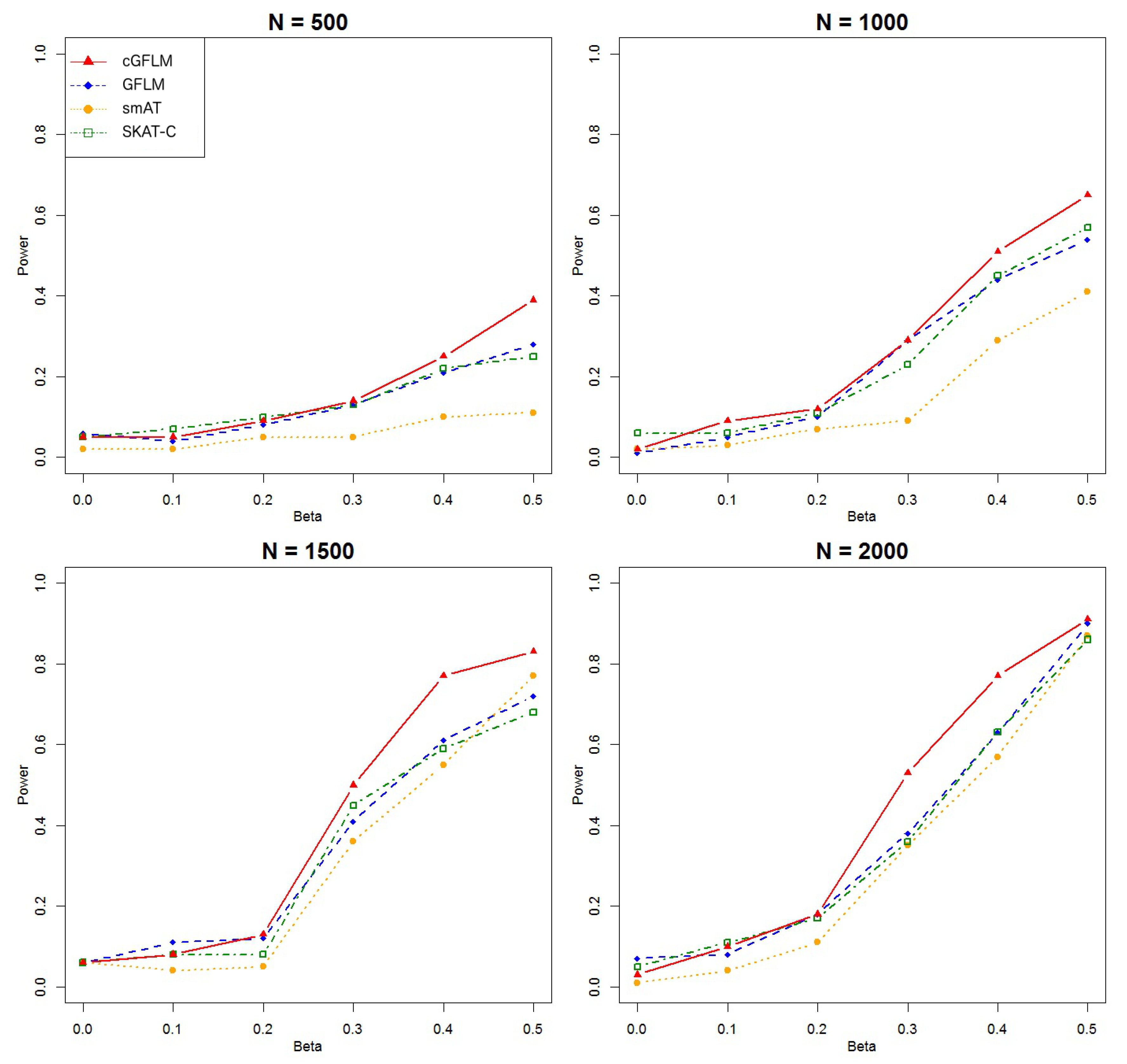
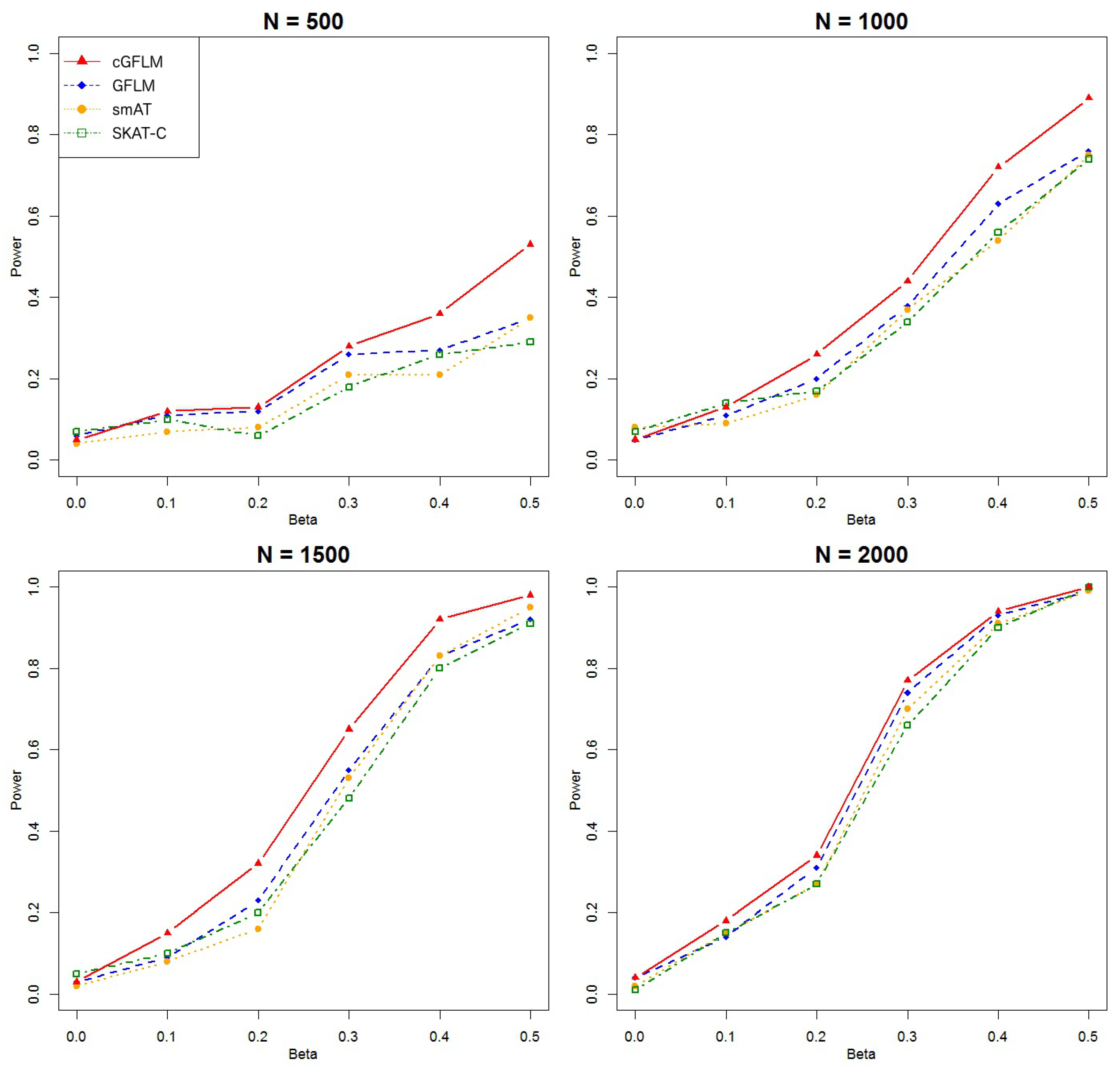
Because the simulation results using the random LD blocks and the LD block structure from CHRNA7 gene are very similar, here we only show results with the random LD blocks, whereas the results with the CHRNA7 gene are located in Appendix A (

Table A1. Type I error simulation using cGFLM for binary outcomes based on the CHRNA7 gene.

Nominal $\mathit{\alpha }$	N = 500	N = 1000	N = 1500	N = 2000
0.05	0.0508	0.0512	0.0493	0.0506
0.01	0.0100	0.0099	0.0102	0.0093
0.005	0.0056	0.0053	0.0048	0.0046
0.001	0.0011	0.0009	0.0011	0.0007

and

Table A2. Type I error simulation using cGFLM-ZINB for ZINB outcomes based on the CHRNA7 gene.

Nominal $\mathit{\alpha }$	N = 500	N = 1000	N = 1500	N = 2000
0.05	0.037	0.046	0.045	0.042
0.01	0.011	0.011	0.006	0.008
0.005	0.005	0.007	0.002	0.006

, Figure A1, Figure A2, Figure A3, Figure A4, Figure A5 and Figure A6). For a random LD block, all SNP genotypes within it were generated following the strategy introduced in [9,11]. Briefly, genotypes of p SNPs were generated based on a random p-dimensional multivariate normal matrix ${\zeta }_{n\times p}$ with mean $\mathbf{0}$ and covariance ${\mathsf{\Sigma }}_{p\times p}$. Assuming that SNPs have equal allele frequencies, the following rule would be applied to generate the genotype of the jth SNP for the ith subject. Let $z_{0.25}$ be the third quartile of standard normal distribution, we have:

$$X_{ij}=\left\{\begin{array}{cc}0,\hfill & \mathrm{if}{\zeta }_{ij}<-z_{0.25}.\hfill \\ 1,\hfill & \mathrm{if}-z_{0.25}\le {\zeta }_{ij}<z_{0.25}.\hfill \\ 2,\hfill & \mathrm{if}{\zeta }_{ij}\ge z_{0.25}.\hfill \end{array}\right.$$

(34)

The covariance matrix was defined as follows. For each block, $10\%$ of the SNPs were selected as “tag SNPs”. They were highly correlated with each other ($Corr(X_{j1},X_{j2})=0.8$), moderately correlated with $30\%$ of other SNPs ($Corr(X_{j1},X_{j2})=0.5$), and weakly correlated with the remaining $60\%$ SNPs ($Corr(X_{j1},X_{j2})=0.2$). The correlations among the $90\%$ “non-tag” SNPs are determined by their physical locations ($Corr(X_{j1},X_{j2})={0.7}^{|j_1-j_2|}$). In this case, we would not violate the assumptions that SNPs are physically adjacent and linked. Further, the LD block structures vary among different randomly generated arrays.

5.1. Simulation Using Binary Traits

The following binary outcomes were simulated based on causal genotypes under the logit model:

$$\mathrm{logit}\left(\mu \left(y_i\right)\right)=\log \frac{Pr(y_i=1)}{1-Pr(y_i=1)}={\alpha }_0+{\mathit{X}}_{\mathit{i}}^{\top }{\mathit{\beta }}_{\mathit{causal}}$$

(35)

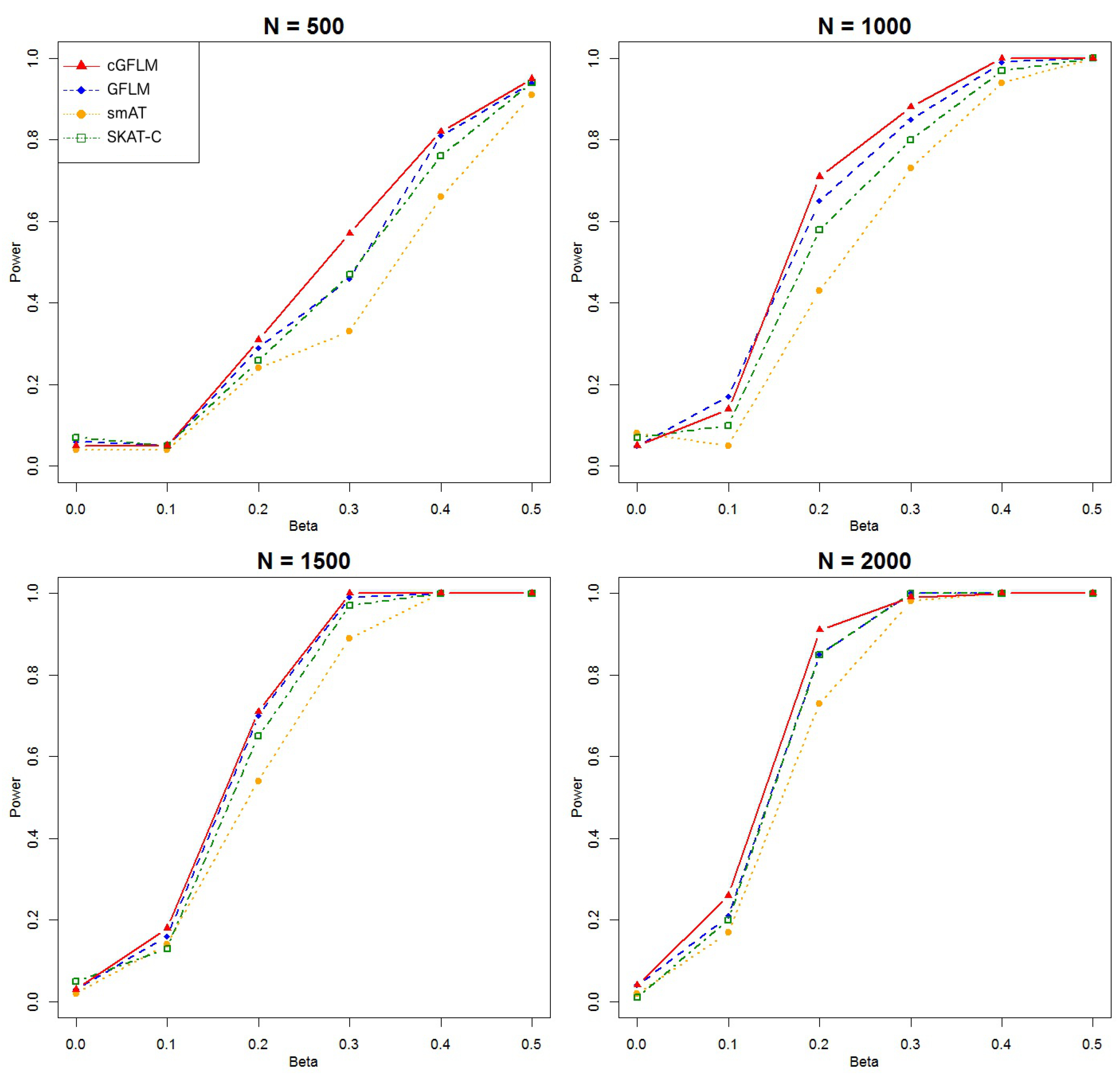
We considered simulation scenarios where ${\alpha }_0=0.2$. Each scenario was replicated 10,000 times in order to observe the type I error rates under small genome-wide thresholds (nominal $\alpha =0.05,0.01,0.005\mathrm{and}0.001$). We ran 1000 replicates for each scenario for power evaluation, in which a p-value smaller than 0.05 would be declared for significance. We compared the empirical power of our proposed model with three existing methods: single marker association test (smAT), SKAT for the combined effect of rare and common variants (SKAT-C) and the functional linear model (GFLM). p-values for smAT were adjusted by Bonferroni correction, and p-values for SKAT-C and GFLM were calculated by combined sum test and ${\chi }^2$ test.

We can see from

Table 1. Type I error simulation using cGFLM for binary outcomes based on randomly generated LD blocks.

Nominal $\mathit{\alpha }$	N = 500	N = 1000	N = 1500	N = 2000
0.05	0.0500	0.0473	0.0466	0.0482
0.01	0.0109	0.0076	0.0099	0.0082
0.005	0.0054	0.0045	0.0046	0.0033
0.001	0.0010	0.0009	0.0011	0.0006

that cGFLM can effectively maintain the type I error. Evaluation of empirical power was based on settings when regression coefficient ${\beta }_{causal}=0.1,0.2,0.3,0.4$ or $0.5$. For power calculation with single causal locus, we used the same settings as that in type I error simulation. When causal SNPs were not genotyped, we can see from Figure 1 that the cGFLM showed better power than all other methods. In the second scenario when two causal loci had reverse-sign effects, we included more SNPs in a block so that it would be possible to locate two weakly correlated markers within the region. We used $p=25$ SNPs in a group and $d_1=d_2=4$ as the number of spline bases. From Figure 2, we can see that cGFLM consistently demonstrates better power than other methods.

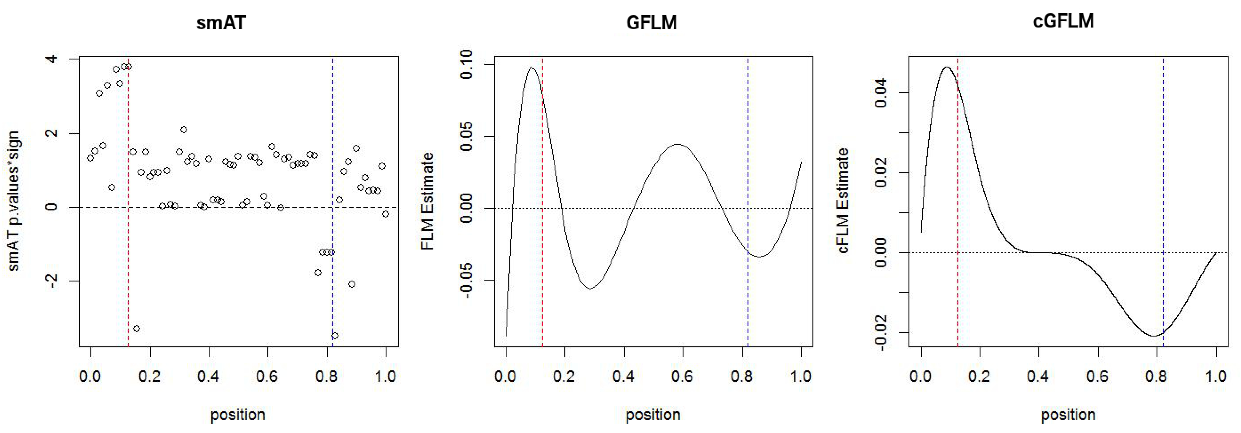
The association patterns of a sample simulation are presented in Figure 3. For smAT, a modified Manhattan plot of the −log10 (p-values) by the sign of the fitted coefficients is used. For all other methods, the coefficient estimates are plotted. The causal loci is highlighted with dashed lines (left in red for positive effect, right in blue for negative effect). Compared to smAT and cGFLM, the cGFLM fitted coefficient function is more reasonable and correctly identify the causal loci.

5.2. Simulation Using ZINB Traits

In this case, we simulate phenotypic traits conditional on causal genotypes under the following ZINB model:

$$\begin{array}{cc}\hfill \mathrm{logit}\left({\pi }_i\right)& =log\frac{{\pi }_i}{1-{\pi }_i}={\alpha }_0^{Ber}+{\mathit{X}}_{\mathit{i}}^{\top }{\mathit{\beta }}_{\mathit{causal}}^{\mathit{Ber}}\hfill \\ \hfill log\left({\mu }_i\right)& ={\alpha }_0^{NB}+{\mathit{X}}_{\mathit{i}}^{\top }{\mathit{\beta }}_{\mathit{causal}}^{\mathit{NB}}\hfill \end{array}$$

(36)

The outcomes are generated with the latent mixture process as discussed in Section 3.

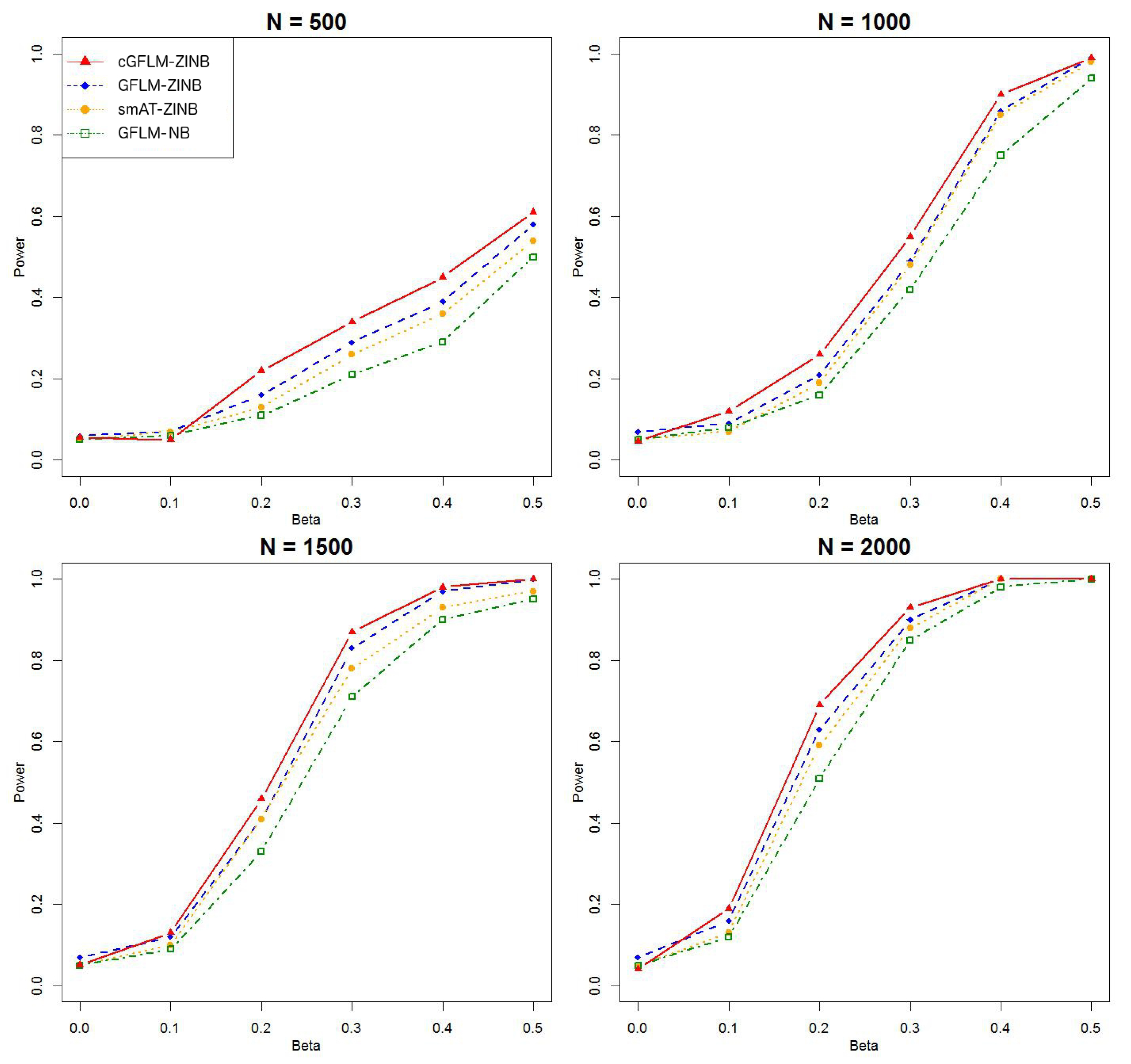
The intercepts, ${\alpha }_0^{Ber}$ and ${\alpha }^{NB}$, were set to be $0.0$ in all subsequent simulations. ${\beta }_{causal}$ was set to zero under the null hypothesis in the evaluation of type I error. Since the computational burden for ZINB models is much higher than that in the binary outcome model, we reduced the replicated times to 1000 times for each scenario. Type I error rates were investigated under small genome-wide thresholds (nominal $\alpha =0.05,0.01\mathrm{and}0.005$). For assessment of empirical power, we used similar settings as those in the simulation for binary traits. However, we examined two general scenarios where the genetic effect is in either the latent Bernoulli or the negative binomial models. Then for each general scenario, we first set only one causal SNP in the LD block, affecting either ${\beta }_{causal}^{Ber}$ or ${\beta }_{causal}^{NB}$. Then we considered two causal loci with reversed sign effects in the LD block. The two causal loci chosen were weakly correlated ($r^2<0.01$). The corresponding regression coefficients were set to $({\beta }_{causal1}^{Ber},{\beta }_{causal2}^{Ber})$, or $({\beta }_{causal1}^{NB},{\beta }_{causal2}^{NB})$ where ${\beta }_{causal1}=-{\beta }_{causal2}$. A total of 100 replicates were run for each scenario. We compared the empirical power of our proposed model cGFLM-ZINB with three existing methods: functional linear model with negative binomial traits (GFLM-NB), single marker association test with ZINB traits(smAT-ZINB) and functional linear model with ZINB traits (GFLM-ZINB). p-values for smAT-ZINB were adjusted by Bonferroni correction, and p-values for GFLM-NB and GFLM-ZINB were calculated by the likelihood ratio tests.

Table 2. Type I error simulation using cGFLM-ZINB for ZINB outcomes based on randomly generated LD blocks.

Nominal $\mathit{\alpha }$	N = 500	N = 1000	N = 1500	N = 2000
0.05	0.055	0.046	0.051	0.040
0.01	0.009	0.009	0.012	0.007
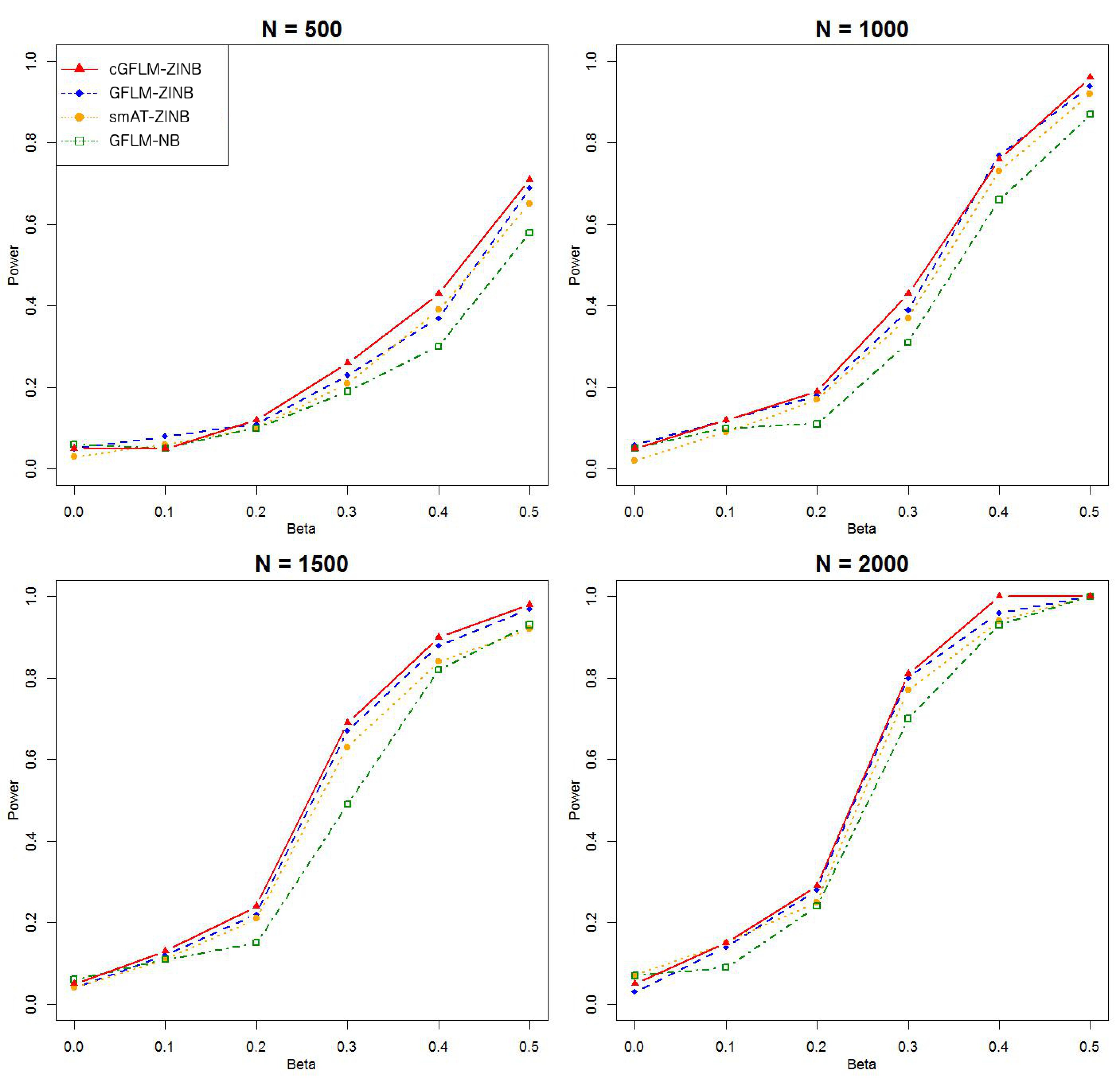
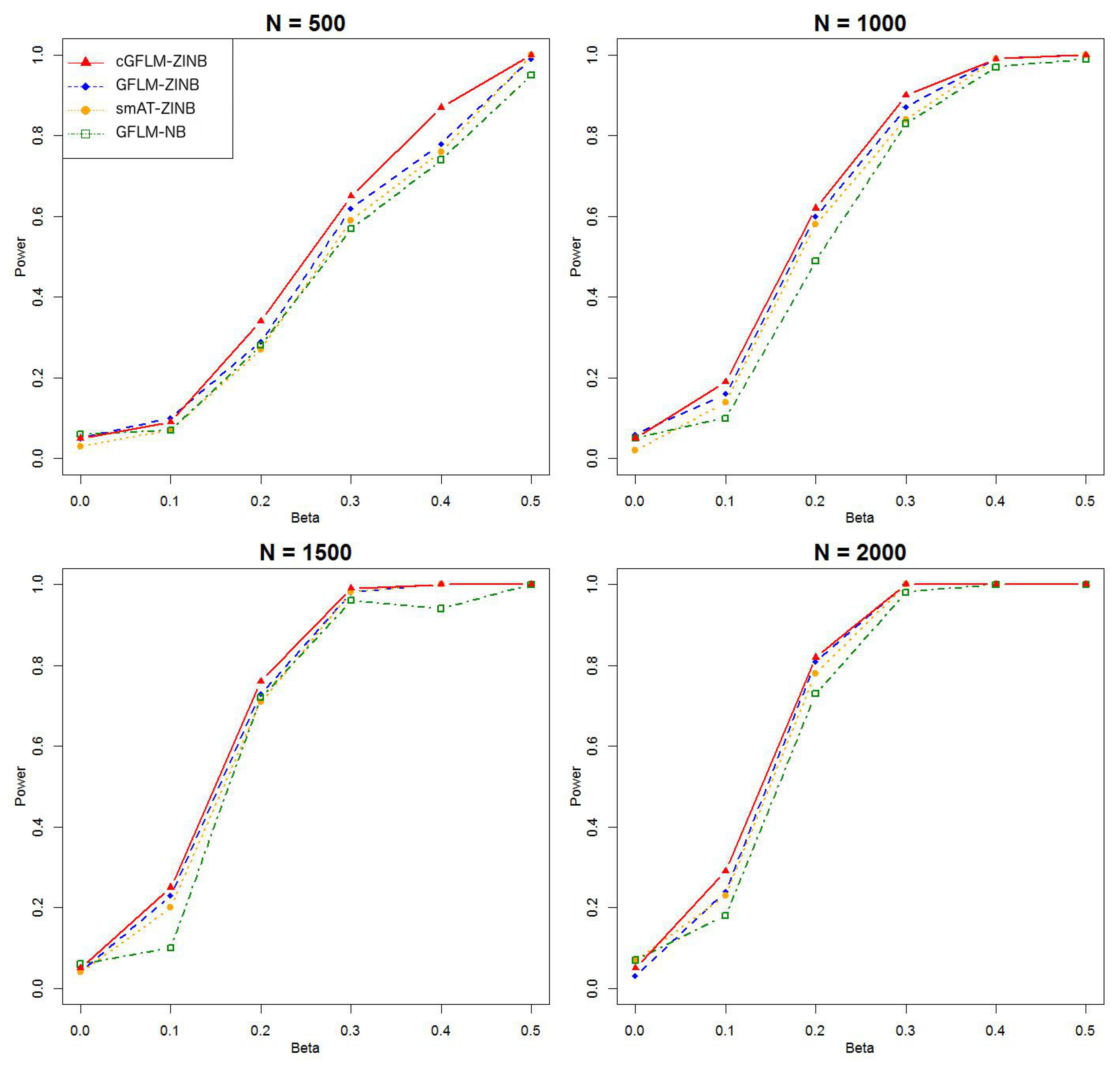
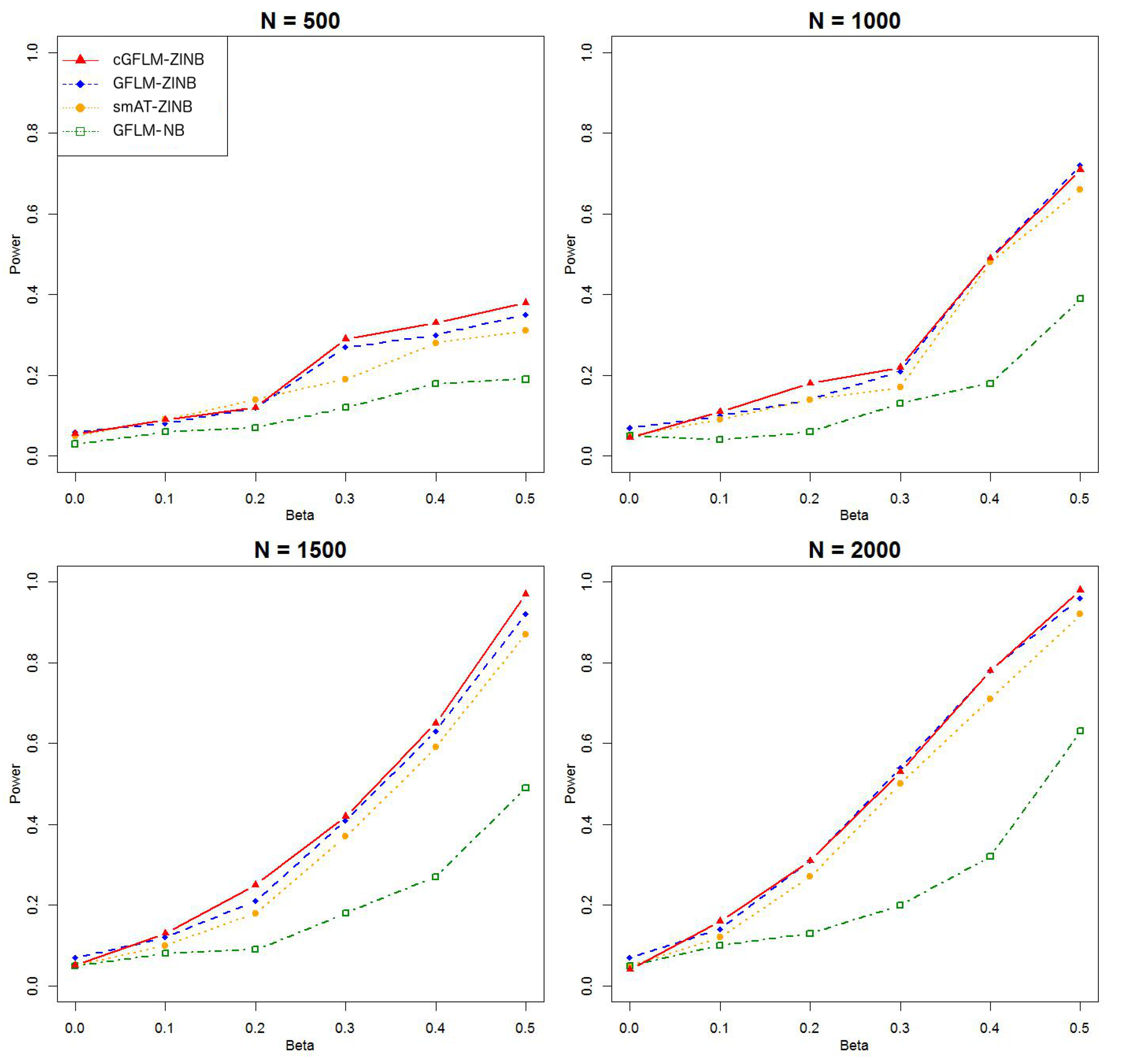
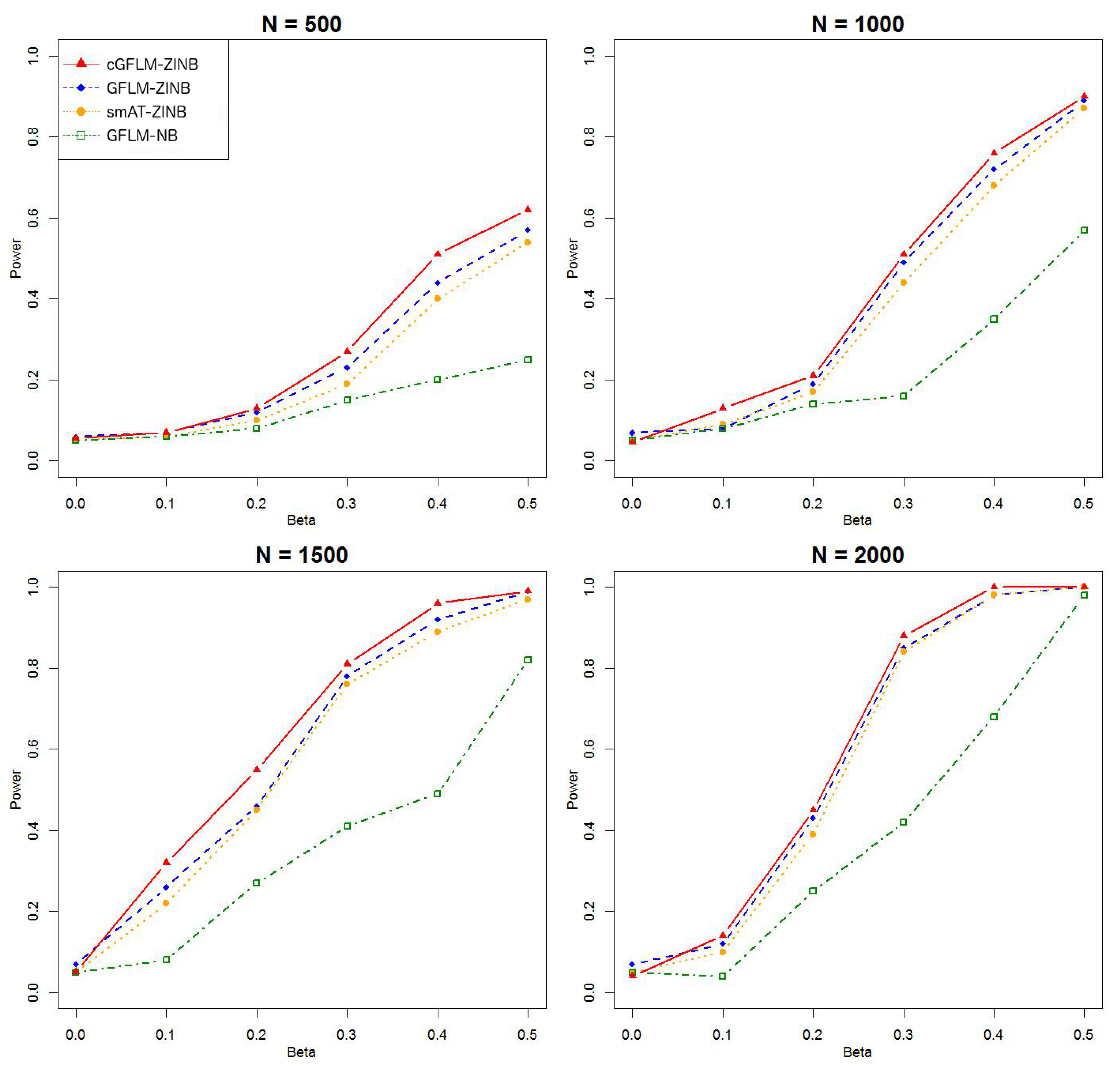
0.005	0.003	0.007	0.008	0.004

demonstrated that the proposed cGFLM maintains the type I errors very well. Evaluation of empirical power is based on settings with regression coefficients ranging from 0.1 to 0.5 and sample sizes from 500 to 2000. When the genetic effect was set to be in the latent Bernoulli model, we can observe the apparent failure of using a negative binomial (NB) regression model, by looking at the significantly lower power when using the GFLM-NB model compared with other models in Figure 4 and Figure 5. This fortifies our assumption that using a simple NB distribution will lead to loss of power when modeling genetic effects affecting excess zero in zero-inflated count process. While using ZINB models, similar performances were observed for smAT-ZINB, GFLM-ZINB and cGFLM-ZINB (see Figure 6 and Figure 7). The figures demonstrate that ZINB models are more advantageous than the NB regression model when excessive zeros exist. More importantly, the cGFLM-ZINB model consistently shows the best performance among the tested models, in scenarios when one causal locus and two causal loci were set in the LD block. Collectively, these simulations demonstrate the advantages and robustness of our proposed cGFLM model.

We then applied the cGFLM model to two independent studies to assess its practical usage. The first dataset is a candidate-gene-based SNP study and the other is a GWAS for dental caries.

6. Application 1: COGEND Study

According to the World Health Statistics Report [25], cigarette smoking is the single biggest cause of preventable mortality worldwide, causing more than 5 million deaths per year and accounting for one in 10 adult deaths. Nicotine dependence, the primary psychoactive component in tobacco, profoundly impacts people’s ability to cease tobacco smoking. The etiology of nicotine dependence is multifactorial, and evidence from various epidemiology studies suggest that genetic factors have a substantial impact on smoking behaviors. Identification of these genetic factors and the development of targeted treatments could be promoted to further reduce smoking related morbidity and mortality.

The Collaborative Genetic Study of Nicotine Dependence (COGEND) is a nationwide project aiming to detect the genetic mechanisms and environmental features of nicotine dependence. In this study on CHRN candidate genes, a total of 216 SNPs were genotyped for 2022 individuals (1114 cases with nicotine dependence and 908 controls). In the phenotypic data, all cases and controls were current or former smokers who reported smoking more than 100 cigarettes lifetime. Rates of current nicotine dependence were defined by the Fagerstrom Test for Nicotine Dependence (FTND). Subjects having FTND $\ge 4$ were classified as nicotine dependent (case). Subjects having lifetime FTND = 0 or 1 were classified as control. The original SNP set was divided into 12 LD blocks according to their physical locations and LD structure, all of which consist of one or more contiguous gene regions. Since functional models are not well-suited for LD blocks having small number of SNPs, four small blocks with fewer than seven SNPs were excluded for analyses. We applied our proposed method cGFLM, along with smAT, SKAT-C and GFLM to analyze the final dataset, which consists of 191 SNPs in eight LD blocks. Age, gender and race were included as covariates. A Bonferroni significance threshold of $0.05/8=6.2\times {10}^{-3}$ is used for cGFLM, GFLM and SKAT-C, and a threshold $0.05/191=2.6\times {10}^{-4}$ is used for smAT.

Table 3. Association tests for COGEND study based on LD blocks using single-marker association tests with Bonferroni correction (smAT), SKAT-C, GFLM and cGFLM.

p-Value LD Block	CHR	Length	# of		p-Value
(Genes)		(kb)	SNPs	cGFLM	smAT	SKAT-C	GFLM
CHRND	2	43	10	0.0990	0.4818	0.1920	0.1321
CHRNA9	4	20	11	0.4308	0.7580	0.3941	0.3915
CHRNA2	8	31	11	0.7078	0.7596	0.5698	0.8036
CHRNB3 + CHRNA6	8	101	25	$8.67\times {10}^{-4}$	0.0064	0.0013	0.0033
CHRNA7	15	126	39	0.2759	0.3382	0.6078	0.5587
CHRNA5 cluster	15	212	72	$5.25\times {10}^{-6}$	$1.72\times {10}^{-4}$	0.0017	$8.24\times {10}^{-6}$
CHRNB1	17	84	14	0.0137	0.3975	0.0274	0.0602
CHRNA4	20	17	9	0.0556	0.1134	0.0255	0.1409

summarizes the results. All four methods yielded small p-values (cGFLM: $5.25\times {10}^{-6}$; GFLM: $8.24\times {10}^{-6}$; SKAT-C: $1.7\times {10}^{-3}$; smAT: $1.72\times {10}^{-4}$) for the CHRNA5 cluster (“IREB2 + LOC123688 + PSMA4 + CHRNA5 + CHRNA3 + CHRNB4” gene cluster) on chromosome 15. However, only cGFLM and SKAT-C showed significance for the “CHRNB3 + CHRNA6” gene cluster (cGFLM: $8.67\times {10}^{-4}$; SKAT-C: $1.3\times {10}^{-3}$). For these two blocks, p-values calculated by cGFLM are much smaller than those calculated by other methods. It is also worth mentioning that both gene clusters have been shown to be associated with nicotine dependence in previous studies [26,27,28,29]. Other LD blocks (candidate gene clusters) are not significantly associated with the phenotypic trait in this cohort.

7. Application 2: Whole Genome Association Study for Dental Caries

More than 40% children and adolescents, and 90% adults in the US are being affected by dental caries, or more commonly known as tooth decay. Multiple factors are considered to contribute to the risk of having dental caries, such as some environmental factors and social behaviors [30,31,32]. Evidence has shown that some individuals are more susceptible to caries while some others are more resistant, almost irrelevant to the environmental risk factors they are exposed to, suggesting that genetic factors may play crucial roles in the risk of developing caries [33]. According to several previous studies, the heritability of dental caries were evaluated to be as high as 60%.

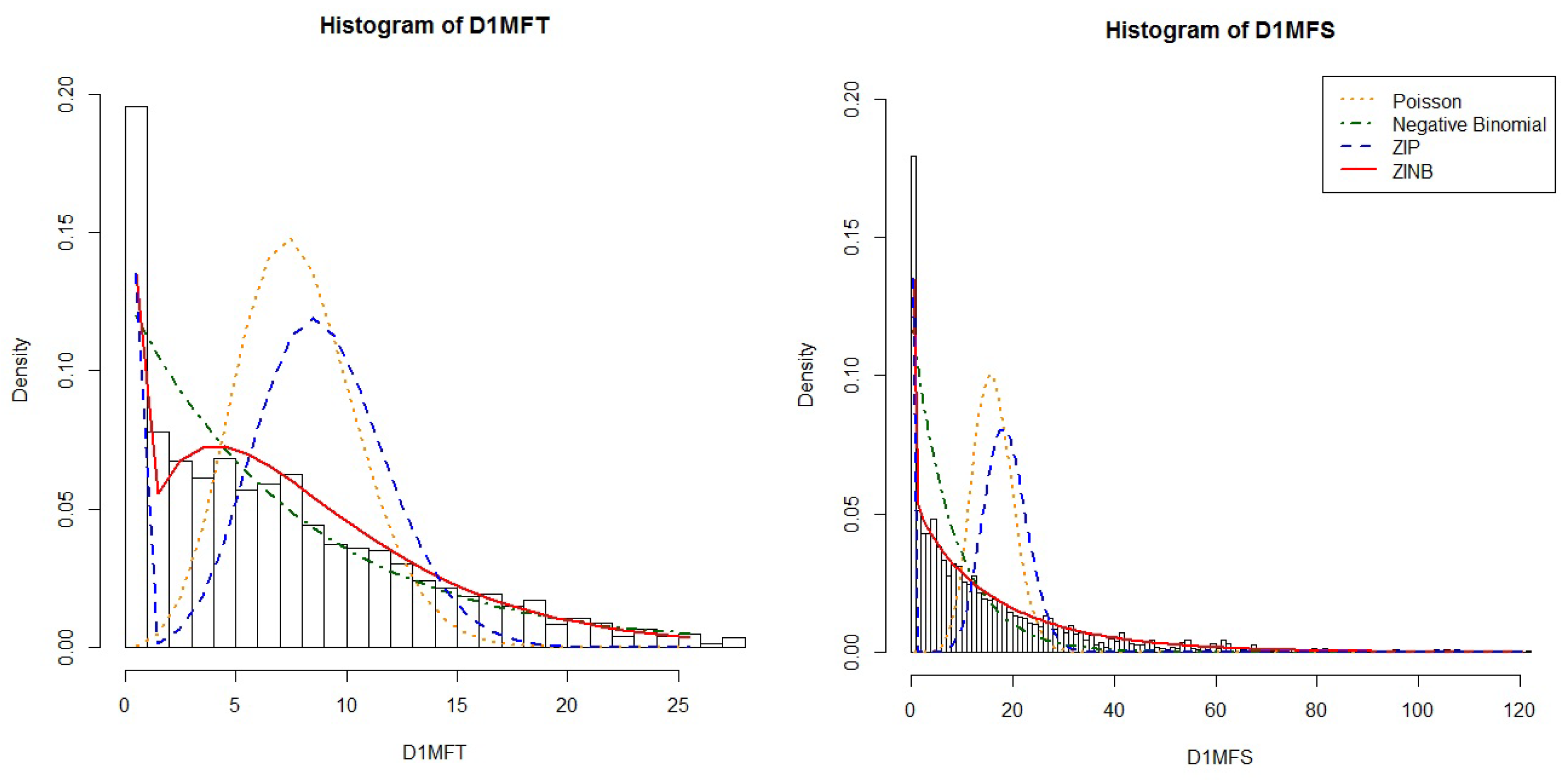
To better understand the genetic mechanisms of the risk of dental caries, a GWAS study has been conducted as part of the Gene Environment Association Studies initiative (deposited in dbGaP Study Accession: phs000095.v2.p1) [4,34]. A total of 4020 individuals were genotyped with a large panel of SNPs (610,000) and examined with multiple outcomes. Our study focused on traits related to caries in permanent teeth. Two indexes, D1MFT and D1MFS, which quantifies the total permanent tooth/surface caries with white spots, were included in the analyses. Since the outcomes of interest were both count traits with excess zeroes (Figure 8), the proposed methods, zero-inflated negative binomial model (smAT-ZINB for single-marker tests) and its application with functional coefficient (GFLM-ZINB and cGFLM-ZINB), were applied to the data set. The final analytic sample consists of 1480 individuals with complete permanent teeth phenotypic data. Age, gender and total number of teeth/surfaces were included as covariates in the analyses.

Table 4. Significant findings for dental caries GWAS scanning using single-marker association tests based on the ZINB model.

		Trait: D1MFT
SNP ID	CHR	Gene	MAF	p-Value
rs7990965	13	-	0.033	$1.02\times {10}^{-12}$
rs1058595	10	PHYH	0.063	$2.52\times {10}^{-9}$
rs12344120	9	-	0.029	$4.79\times {10}^{-8}$
rs4694666	4	MTHFD2L	0.135	$5.48\times {10}^{-8}$
rs17078140	3	LIMD1	0.029	$5.77\times {10}^{-8}$
rs9893536	17	USP32	0.091	$8.80\times {10}^{-8}$
rs7334525	13	RFC3	0.093	$9.52\times {10}^{-8}$
		Trait: D1MFS
SNP ID	CHR	Gene	MAF	p-Value
rs7990965	13	-	0.033	$2.40\times {10}^{-10}$
rs1058595	10	PHYH	0.063	$3.29\times {10}^{-9}$

and

Table 5. Significant findings for dental caries association tests based on LD blocks (gene clusters) using the ZINB model (smAT-ZINB with Bonferroni correction, GFLM-ZINB, cGFLM-ZINB).

		Trait: D1MFT
LD Block	CHR	Length	# of		p-Value
(Genes)		(kb)	SNPs	cGFLM	GFLM	smAT
PKDCC	2	70	18	$8.41\times {10}^{-7}$	$8.06\times {10}^{-5}$	$4.17\times {10}^{-5}$
		Trait: D1MFS
LD Block	CHR	Length	# of		p-Value
(Genes)		(kb)	SNPs	cGFLM	GFLM	smAT
Intergenic between DCN and BTG1	12	70	21	$6.07\times {10}^{-7}$	$5.92\times {10}^{-6}$	$4.41\times {10}^{-3}$
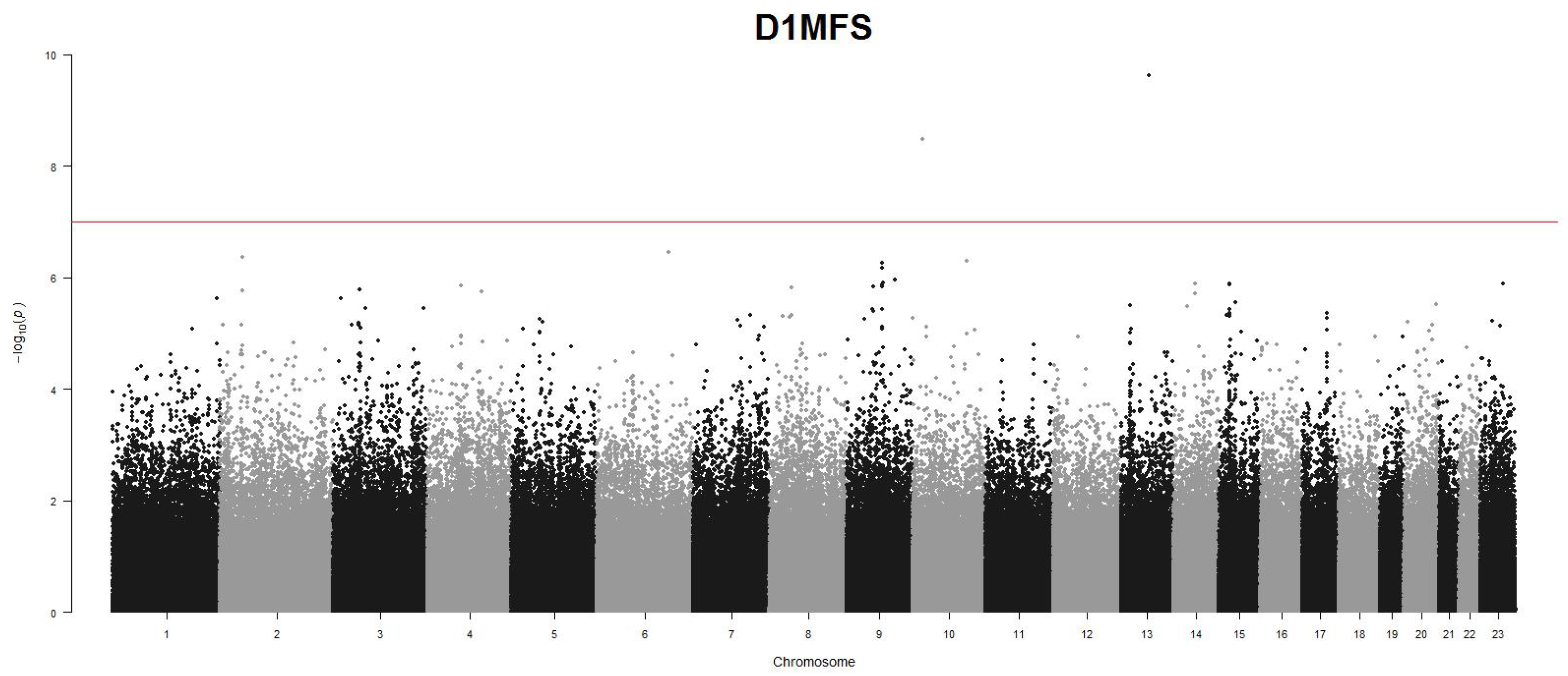
PKDCC	2	70	18	$1.38\times {10}^{-6}$	$1.59\times {10}^{-4}$	$7.73\times {10}^{-6}$

summarize the significant findings. The Manhattan plots for GWAS scans using the ZINB model are presented in Figure 9 and Figure 10. For genome-wide univariate screening, a significance threshold of $1\times {10}^{-7}$ was used. For the LD block-based analysis, a genome-wide significance threshold of $2.5\times {10}^{-6}$ was used. Several SNPs were identified significantly associated with D1MFT and D1MFS in genome-wide scan, of which rs7990965 in chromosome 13 and rs1058595 in chromosome 10 demonstrate consistent significance for both traits. In the LD block based association tests, the cGFLM-ZINB model identified two significant genetic regions: PKDCC in chromosome 2 ( both traits), and the intergenic region between DCN and BTG1 in chromosome 12 (D1MFS). It is worth mentioning these two genetic regions cannot be identified by other competing methods, suggesting that the cGFLM model may provide potentially new insights into understanding the risk of dental caries. More interestingly, the gene PKDCC was found to be associated with craniofacial morphogenesis in previous dental studies [35], further supporting and validating the biological significance of our findings.

8. Discussion

Joint analyses of multiple contiguous SNPs, which can form an LD block, are expected to provide better inference about unknown causal variants, since these SNPs all carry partial information about the causal variants and collectively they should be more powerful. In principle, LD between genetic loci should decline with their intervening physical distance, given that more cross-over events occur within longer ranges. Therefore, how to effectively incorporate and take full advantage of the distance/alignment order information of these SNPs is an important yet challenging problem. While FLMs seem to provide a good solution, its estimated coefficient function is usually noisy and hard to interpret, which consequently leads to potential power loss. Improvements to existing methods are then of great interest in order to better detect significant genetic variants.

In this article, we proposed a novel cGFLM for flexible and more reasonable multi-loci mapping strategy. Our model is built upon the general FLM framework by imposing constraints to specify sign-specific effects. Our limited simulations suggest that these constraints encourage spatial sparsity in the estimated coefficient function, which needs to be further validated in other experimental settings. Due to these constraints, the likelihood ratio test statistic does not follow a fixed chi-square distribution, but a null weighted mixture of chi-square distributions. The simulation results show that compared to three competing methods, our proposed cGFLM generally demonstrated better power when effect size is moderate and large, and comparable performance when effect size is small, while at the same time maintaining correct type I errors.

Applications of the cGFLM to two real datasets demonstrate the applicability of our method. Particulary, its application to the GWAS of dental caries risk identifies new genetic regions that are have not been discovered before, validating that our method can potentially provide new insights into large-scale genomic studies. However, it is also important to note that some significant SNPs identified by other methods were missed by cGFLM as well. This is likely because in cGFLM, identification of significant SNPs is based on the collective evidence of a group of linked SNP, and in the case of causal SNPs being weakly linked to its neighboring SNPs, our methods may miss them. Additionally, cGFLM inherently would not work well for variants not in LD with neighboring SNPs, such as singletons and doubletons. Therefore, these observations suggest that our method should be considered as an additional approach in our toolbox for more discoveries, while not replacing existing ones.

When the cGFLM method is applied to large-scale genome-wide scanning of LD blocks, one concern is how to group SNPs into LD blocks. Several software, such as PLINK [36] and LDExplorer [37], have embedded functions to define LD blocks for genomic data, and we can utilize them to help partition the genome. Even with these tools, LD blocks can vary with different LD thresholds. That is, a weaker LD threshold can lead to larger LD blocks and vice versa. Another concern is about LD blocks with few SNPs, since they are not suitable for functional analysis. They can be either combined into adjacent larger blocks with weak LD, or can be just analyzed with those single-marker methods. Prospectively, in order to discover the core subset of causal genes, further group selection among multiple candidate blocks is of great interest, and regularization methods such as group LASSO and group SCAD can be included as extensions to our current framework. Additionally, in this study cGFLM only considers LD-based blocks for association analyses; however, it would be also of great interest to see if cGFLM can be applied to gene-level analyses as genes are functional units of the genome. Finally, if subpopulations exist in the genotypic sample, stratification can be addressed in our model by including principal components of population variation as additional covariates [38].

9. Conclusions

Our proposed GFLM, cGFLM and their related implementations with the ZINB model (GFLM-ZINB, cGFLM-ZINB) are novel and complex methods. They are specifically designed for multi-loci mapping in naturally formed LD blocks. The models can simultaneously incorporate multiple linked SNPs, including their physical alignments and block-wide linkage structure, and make inference at the LD block level. Simulation studies show that cGFLM and cGFLM-ZINB have desirable performances in terms of both simpler coefficients functions and empirical power gain. The practical usage of cGFLM is demonstrated with a candidate-gene study of nicotine dependence and a GWAS on dental caries. Considering its flexibility and comprehensiveness, cGFLM would be a very attractive method for future gene-based association studies.