Article

Normality Testing of High-Dimensional Data Based on Principle Component and Jarque–Bera Statistics

1
School of Mathematics and Statistics, Lanzhou University, Lanzhou 730000, China
2
School of Mathematics and Statistics, Xi’an Jiaotong University, Xi’an 710049, China
*
Author to whom correspondence should be addressed.
Stats 2021, 4(1), 216-227; https://doi.org/10.3390/stats4010016
Submission received: 28 January 2021 / Revised: 10 March 2021 / Accepted: 12 March 2021 / Published: 17 March 2021
(This article belongs to the Section Computational Statistics)

Abstract

:
The testing of high-dimensional normality is an important issue and has been intensively studied in the literature, it depends on the variance–covariance matrix of the sample and numerous methods have been proposed to reduce its complexity. Principle component analysis (PCA) has been widely used in high dimensions, since it can project high-dimensional data into a lower-dimensional orthogonal space. The normality of the reduced data can then be evaluated by Jarque–Bera (JB) statistics in each principle direction. We propose a combined test statistic—the summation of one-way JB statistics upon the independence of the principle directions—to test the multivariate normality of data in high dimensions. The performance of the proposed method is illustrated by the empirical power of the simulated normal and non-normal data. Two real data examples show the validity of our proposed method.

1. Introduction

Normality plays an important role in statistical analysis and there are numerous methods for normality testing presented in the literature. Koziol [1] and Slate [2] used the properties of normal distribution function to assess multivariate normality. Reference [3] checked normality using a class of goodness-of-fit tests and this kind of method was also discussed in [4,5]. Various statistics have also been used in recent years, such as the Cramér-Von Mises(CM) statistic [5], skewness and kurtosis [6], sample entropy [7], Shapiro–Wilk’s W statistic [8] and the Kolmogorov-Smirnov(KS) statistic (see also in [9,10,11]).
It is noticed that many studies of the aforementioned statistics are based on univariate normality, while the practical research we concentrate on is based on multivariate normality. Therefore, generalization should be used to enlarge the conclusions from univariate to multivariate. This is a common practice in multivariate normality testing when some useful statistics are adopted. Projection methods such as principle component analysis (PCA) can be exploited to obtain such achievement, as described in [8,12]. Convenient principle component analysis can project a high dimensional dataset into several lower dimensions in independent directions, then statistical tests in each direction can be summarized together to give a total test for multivariate normality, using the fact that the joint probability distribution is the product of all marginal probability distributions for independent variables. With the help of these orthogonal projections, the dimension can be reduced and the computation can be more efficient.
In this paper, the Jarque–Bera statistic, a combination of skewness and kurtosis, instead of the two statistics, as in [8], is investigated to test the normality in each principle direction. Then, a new kind of statistic J B s u m is constructed to test the high-dimensional normality. The performance of the proposed method and its empirical power of testing are illustrated based on some high-dimensional simulated data.
This paper is organized as follows—Section 2 provides the theory of principle component analysis and gives the methodologies of statistical inference for multivariate normality. In Section 3, some simulated examples of normal data and non-normal data are used to illustrate the efficiency of our proposed method. Two real examples are then investigated in Section 4 to verify the methods’ effectiveness.

2. High-Dimensional Normality Test Based on PC-Type JB Statistic

For observed data X = ( x i j ) n × p with sample size n and dimension p, the principle component analysis reduces the dimension of p-variate random vector X through linear combinations, and it searches the linear combinations with larger spread among the observed value of X , i.e., the larger variances. Specifically, it searches for the orthogonal directions ω i ( i = 1 , 2 , , p ) , which satisfy
ω = arg max ω Var ( X ω ) = arg max ω ω T Var ( X ) ω , s . t . ω T ω = 1 .
Denoted by Σ , the covariance matrix of X , the eigenvalue λ i and principle components ω i ( i = 1 , 2 , , p ) can be obtained by spectral decomposition of the covariance matrix Σ . Therefore, the observed data can be projected to the archived lower-dimension space { ω 1 , ω 2 , , ω p } by z i = X ω i , which gives the projected observed matrix z .
For each z i , the skewness and kurtosis can be calculated by
S k z i = 1 n j = 1 n z i j z ¯ i 3 1 n j = 1 n z i j z ¯ i 2 3 / 2 ,
K u z i = 1 n j = 1 n z i j z ¯ i 4 1 n j = 1 n z i j z ¯ i 2 2 ,
where z ¯ i stands for the sample mean. Then, the univariate JB statistic can be given by
J B ( z i ) = n 6 S k 2 z i + K u z i 3 2 4 .
To test the normality of high-dimensional data, z = ( z 1 , z 2 , , z r ) , define
J B s u m ( z ) = i = 1 r J B ( z i ) ,
where r stands for the number of principle components ultimately selected, which satisfies:
i = 1 r λ i i = 1 p λ i 1 s .
Considering the hypothesis:
H 0 : t h e   d a t a   i s   n o r m a l l y   d i s t r i b u t e d ; v . s . H 1 : t h e   d a t a   i s   n o n n o r m a l l y   d i s t r i b u t e d
Under the null hypothesis H 0 , the JB statistic will be asymptotically χ 2 2 distributed [13], then the J B s u m will be asymptotically χ 2 2 r distributed. For a given significance α , the critical region will be
R ( Z ) = { Z | J B s u m ( Z ) > χ α 2 ( 2 r ) } .
Upon J B s u m , an exact critical region R ( X ) can be deduced, and therefore the testing can be implemented based on these critical regions.
Evaluating the performance of the proposed PC-type Jarque–Bera testing depends on (1) whether the orthogonal axes are chosen due to the cumulative proportion; and (2) whether the hypothesis is rejected or accepted. Composed by the well known power function, the error will be:
P o w e r = α with H 0 1 [ ( s + ( 1 s ) β ) ] = ( 1 s ) ( 1 β ) with H 1 ,
where α is the probability of a Type-I error and β is the probability of a Type-II error. Therefore, we can see that the power is a non-decreasing function of the parameter s.

3. Numerical Simulations

To evaluate the performance of the aforementioned testing, some simulation experiments are carried out in this section.

3.1. Normally Distributed Data

A series of normally distributed data were investigated with different data dimension p and different sample size n. Let n × p simulated data matrix X n × p N μ , Σ , where μ = 0 . Consider two kinds of covariance matrix:
(I)
Σ = ρ I ( i j 0 ) ;
(II)
Σ = 0.5 ρ I ( i j 0 ) + 0.5 ρ | i j | .
Define
Empirical power = n false / n normal ,
where n f a l s e is the number of rejected samples, n n o r m a l is the number of samples that obey the normal distribution. Table 1, Table 2, Table 3, Table 4, Table 5 and Table 6 describe separately the Empirical power of the PC-type JB testing J B s u m compared with S k -type statistics χ s k 2 , S k m a x [14], K u -type statistics χ k u 2 , K u m a x [14], Mardia’s method Z M 1 * [15], Srivastava’s method Z S 1 * [16], Kauyuki’s method M J B m * , M J B s * [16], Kazuyuki’s method m J B M [17] in these two cases with significance level α = 0.01, 0.05, 0.10 respectively.
From the table above we can conclude that in the case of normal data, the empirical power of J B s u m is small and stable whenever p / n is large or small. Although the empirical power of each statistic converges to the given significance level as n increases, the performance of S k m a x (especially when α = 0.1), K u m a x , Z M 1 * , M J B m * and Z N T is not so good as p increase. Besides, it is noticed that Z S 1 * , M J B s * and m J B M are inapplicable to p > n whereas J B s u m still works well. For all six tables, the numbers in bold represent the empirical power that is closest to the significance level among the eleven statistics in each situation.

3.2. Non-Normally Distributed Data

In this part, non-normal datasets are simulated to evaluate the performance of the proposed method according to Empirical power. Define
Empirical power = n true / n non normal ,
where n t r u e is the number of accepted samples, n n o n n o r m a l is the number of samples that do not obey the normal distribution. The performance is evaluated in three databases as follows:
(III)
S h i f t e d χ 2 1 : every variable in X n × p was centralized, with independently identical distribution χ 2 1 .
(IV)
S h i f t e d e x p 1 : every variable in X n × p was centralized, with independently identical distribution e x p 1 .
(V)
N ( 0 , 1 ) + χ 2 2 : the first p / 2 variables in X n × p are from N 0 , 1 distribution, while the last p p / 2 variables independently identically distributed from χ 2 2 , where p / 2 stands for the integer part of p / 2 .
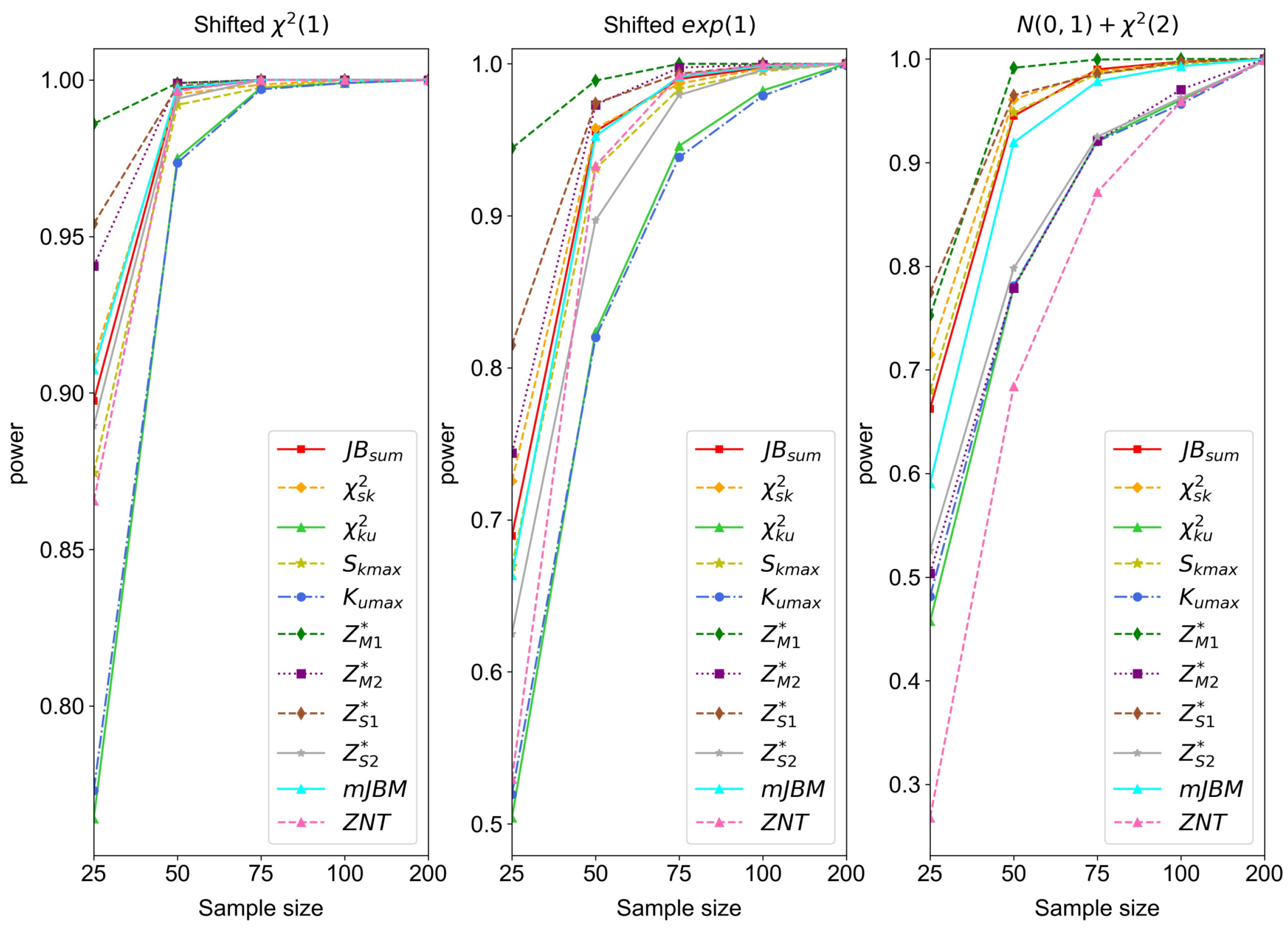
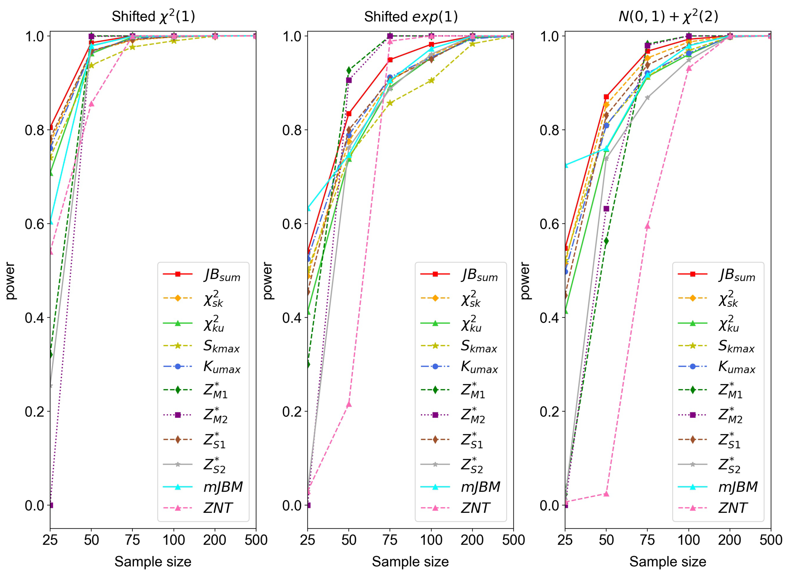
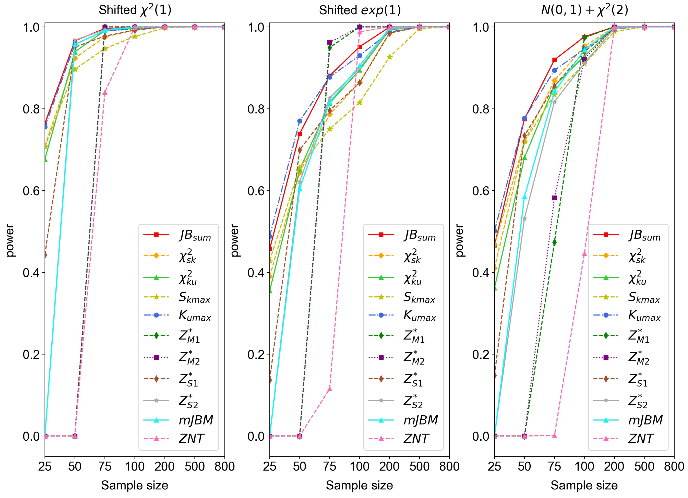
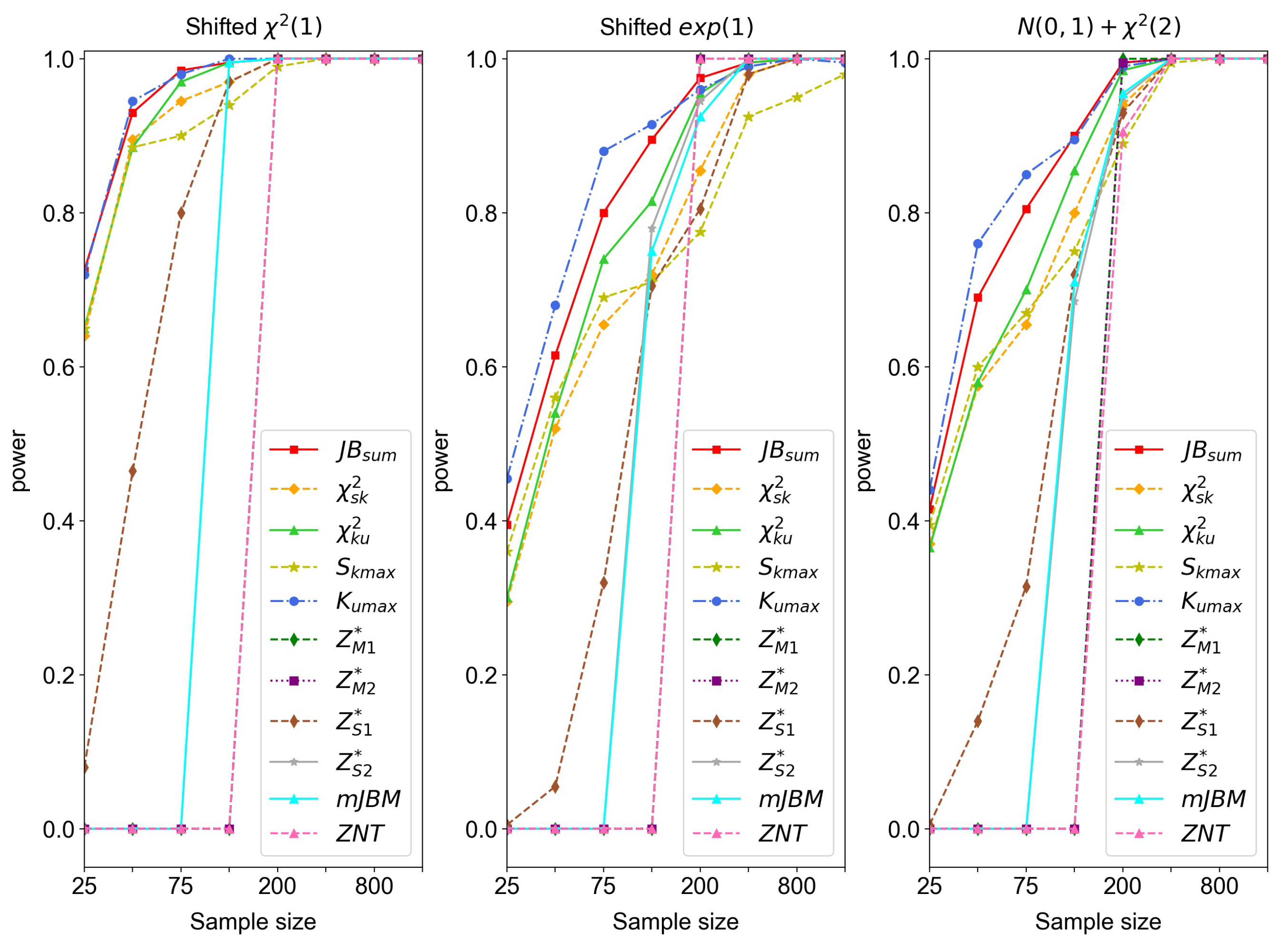
The performance of J B s u m compared with the S k -type statistics χ s k 2 , S k m a x [14], K u -type statistics χ k u 2 , K u m a x [14], Mardia’s statistics Z M 1 * , Z M 2 * [15], Srivastava’s statistics Z S 1 * , Z S 2 * [16], Kazuyuki’s statistic m J B M [17] and Rie’s statistic Z N T [18] are illustrated in Figure 1, Figure 2, Figure 3, Figure 4 and Figure 5. Since J B s u m , χ s k 2 , and χ k u 2 are based on the sum of χ 2 , we call them s u m -type. S k m a x and K u m a x come from the maximum of χ 2 , and thus we call them m a x -type.
All of these methods are studied in 2000 simulated data. Figure 1, Figure 2, Figure 3, Figure 4 and Figure 5 show the comparisons of the empirical power of different dimension p and various sample size n.
(1)
Figure 1 indicates that in the case of p = 5 , Z M 1 * ’s performance is best in all three cases. Though Z M 2 * performs well in Case I and Case II, it is not as good in Case III. Comparatively, Z S 1 * , χ s k 2 and J B s u m perform similarly well and better than χ k u 2 and K u m a x .
(2)
In the case of p = 30 , as in Figure 2, although Z M 1 * and Z M 2 * perform better than J B s u m in Case II, they do not maintain stable results like J B s u m in Case III. In fact, J B s u m ’s performance is generally better than the other methods mentioned here among all three cases.
(3)
In Figure 3, where p = 50 , J B s u m ’s performance is best among others except Z M 1 * and Z M 2 * . As in Figure 2, Z M 1 * and Z M 2 * are unstable in Case III when p is close to n. This phenomenon can also be seen in m J B M . Combining the information shown in Figure 2, we can see that Z M 1 * , Z M 2 * , and m J B M are not as stable as J B s u m .
(4)
With the increase in dimension, as seen in Figure 4, Z M 1 * and Z M 2 * no longer perform as well as before, and m J B M is still not stable enough when n is close to p. Although K u m a x ’s performance is better than J B s u m ’s at first, it is surpassed by the latter when n > 100 .
(5)
In Figure 5, as in p = 100 , the power of K u m a x is initially higher than J B s u m , and is eventually surpassed by J B s u m . Except for K u m a x , J B s u m ’s performance is the best.
From the phenomenon above, we may conclude that J B s u m performs well compared to the other statistics, in that its empirical power is relatively higher than the others and the corresponding simulation results are more stable. Thus, it can be used to test the non-normality of low- or high-dimensional data effectively.

4. Two Real Examples

In this section, we investigated two real examples to illustrate the performance of our proposed method compared with the nine aforementioned existing methods.

4.1. Spectf Heart Data Example

The SPECTF heart dataset [19] provides data on cardiac single proton emission computed tomography (SPECT) images. It describes the diagnosis of cardiac single proton emission computed tomography (SPECT) images, and each patient is classified into two categories: normal and abnormal. The data contain 267 instances, with each instance belonging to a patient along with 44 continuous feature patterns summarized from the original SPECT images. The other attribute is a binary variable that indicates the diagnosis of each patient, with 0 for normal and 1 for abnormal.
In this dataset, we simultaneously evaluate the normality of the whole dataset and each class within it. The testing p-value of each method mentioned above is shown in Table 7. The highest p-value of each relatively normal data set and the lowest p-value of each relatively non-normal data set are in bold.
Let S 0 describe the whole data set and S 1 and S 2 denote the normal class dataset and abnormal class dataset, respectively. We calculate the p-values of our PC-type statistic as well as the S k -type and K u -type statistics and other methods mentioned in [16,17] of these three datasets. Since all ten statistics’ p-values of data S 0 and S 1 are very close to 0, we will not describe them here, which indicates a non-normal distribution of the whole dataset and abnormal dataset.
We may see from Table 7 that S 2 ’s corresponding p-values are a little different from the former two sets, in which the p-values of χ s k 2 , Z M 1 * and M J B M * depart from 0. The relatively high p-values motivate us to conduct a detailed survey to investigate the normality of the SPECTF heart data’s normal class by selecting some kinds of different variables that belong to a variety of degrees of normality.
In this normal category, we extract some variables and construct a new dataset S 3 from several experiments. The selected variables included in S 3 are X 2 , X 4 , X 6 , X 7 , X 9 X 12 , X 14 X 21 , X 23 X 28 , X 31 X 34 , and X 37 X 43 . We then compute the p-values of this dataset, and the results are shown in Table 7. It can be seen that all normality testing methods have a relatively high p-value, which demonstrates the multivariate normality of set S 3 . For comparison, we constructed another two datasets, S 4 and S 5 , which consist of several verified normal variables and non-normal variables, respectively. Specifically, S 4 contains the variables X 3 , X 5 , X 6 X 8 , X 11 X 14 , X 17 , X 21 , X 22 , X 27 X 32 , X 35 , X 36 , X 38 , X 40 , X 43 , and X 44 , while S 5 contains variables X 3 X 8 , X 13 , X 15 , X 22 , X 29 , X 30 , X 35 , X 36 , X 42 , and X 44 . From Table 7 we can see the results of these two sets. This time, the p-values of the ten methods are no longer as high as before, meaning that our method performs well in assessing the normality of normal and non-normal data.

4.2. Body Data Example

In this part, we analyze the normality of body data investigated in [14] to show the consistency of our method with other existing methods and conclusions before. This data set contains 100 human individuals and each individual has 12 measurements of the human body (see [14] for details). As before, the p-values of the PC-type statistics and the S k -type, K u -type, and Kazuyuki’s statistics are computed.
Let B 0 describe the whole dataset, and the multivariate normality of it can be investigated by the resulting p-values of each method shown in Table 7. Since all the p-values approach 0, we may conclude that this dataset contains non-normal data. As with the discussion in [14], we also investigate the other six datasets to show the validity of our proposed method, as well as making a comparison with other methods. For convenience, we denote B 1 = X 1 , X 3 , X 8 , X 10 , X 12 , B 2 = X 1 , X 3 , X 8 , X 10 , B 3 = X 1 , X 8 , X 10 , X 12 , B 4 = X 3 , X 8 , X 10 , X 12 , B 5 = X 4 , X 5 , X 6 , X 11 , and B 6 = X 2 , X 4 , X 6 , X 11 . From Table 8, we can conclude that the normality testing results of our proposed PC-type statistic J B s u m are nearly the same as those for S k -type statistics, K u -type statistics, and Kazuyuki’s methods. Since B 1 , B 2 , B 3 , and B 4 have multivariate distribution, whereas B 5 and B 6 have non-normal distribution [14], our method is closer to the truth in the sense of relatively higher p-values in multivariate normal situations and lower p-values in non-normal situations. Same as in Table 7, the highest p-value of each normal data set and the lowest p-value of each non-normal data set are in bold.
This phenomenon indicates that our proposed PC-type statistic J B s u m constitutes an effective way of testing normality both in normal data and non-normal data, with more stable testing results.

5. Conclusions

The purpose of this paper is to use a JB-type testing method to test high-dimensional normality. The statistics we proposed here used the generalized statistic J B s u m of JB statistics to test normality based on the dimensional reduction performed by PCA.
Through simulated experiments, we find that, in both low and high dimensions, J B s u m performs well in testing normal and non-normal data and it is more stable than many other compared methods. Therefore, it can be used to test normality effectively.
From two real examples, we can also see that our proposed method possesses the superiority of stability in performing the normality testing of real datasets, as well as the inclination of detecting the true normality from the perspective of p-values.

Author Contributions

Data curation, Y.S.; Methodology, X.Z.; Project administration, X.Z.; Software, Y.S.; Supervision, X.Z. All authors have read and agreed to the published version of the manuscript.

Funding

This research was funded by National Natural Science Foundation of China (No. 11971214, 81960309), sponsored by the Scientific Research Foundation for the Returned Overseas Chinese Scholars, Ministry of Education of China, and supported by Cooperation Project of Chunhui Plan of the Ministry of Education of China 2018.

Institutional Review Board Statement

Not applicable.

Informed Consent Statement

Not applicable.

Data Availability Statement

The study used publicly available data from the UC Irvine Machine Learning Repository, https://archive.ics.uci.edu/ml/datasets/SPECTF+Heart.

Acknowledgments

The authors would also like to thank Edit-in-chief and the referees for their suggestions to improve the paper.

Conflicts of Interest

The authors declare no conflict of interest.

References

  1. Koziol, J.A. On assessing multivariate normality. J. R. Stat. Soc. 1983, 45, 358–361. [Google Scholar] [CrossRef]
  2. Slate, E.H. Assessing multivariate nonnormality using univariate distributions. Biometrika 1999, 86, 191–202. [Google Scholar] [CrossRef]
  3. Romeu, J.L.; Ozturk, A. A comparative study of goodness-of-fit tests for multivariate normality. J. Multivar. Anal. 1993, 46, 309–334. [Google Scholar] [CrossRef] [Green Version]
  4. Székely, G.J.; Rizzo, M.L. A new test for multivariate normality. J. Multivar. Anal. 2005, 93, 58–80. [Google Scholar] [CrossRef] [Green Version]
  5. Chiu, S.N.; Liu, K.I. Generalized cramér-von mises goodness-of-fit tests for multivariate distributions. Comput. Stat. Data Anal. 2009, 53, 3817–3834. [Google Scholar] [CrossRef] [Green Version]
  6. Small, N.J.H. Marginal skewness and kurtosis in testing multivariate normality. J. R. Stat. Soc. Ser. (Appl. Stat.) 1980, 29, 85–87. [Google Scholar] [CrossRef]
  7. Zhu, L.-X.; Wong, H.L.; Fang, K.-T. A test for multivariate normality based on sample entropy and projection pursuit. J. Stat. Plan. Inference 1995, 45, 373–385. [Google Scholar] [CrossRef]
  8. Liang, J.; Tang, M.-L.; Chan, P.S. A generalized shapiro-wilk w statistic for testing high-dimensional normality. Comput. Stat. Data Anal. 2009, 53, 3883–3891. [Google Scholar] [CrossRef]
  9. Doornik, J.A.; Hansen, H. An omnibus test for univariate and multivariate normality. Oxf. Bull. Econ. Stat. 2008, 70, 927–939. [Google Scholar] [CrossRef]
  10. Horswell, R.L.; Looney, S.W. A comparison of tests for multivariate normality that are based on measures of multivariate skewness and kurtosis. J. Stat. Comput. Simul. 1992, 42, 21–38. [Google Scholar] [CrossRef]
  11. Tenreiro, C. An affine invariant multiple test procedure for assessing multivariate normality. Comput. Stat. Data Anal. 2011, 55, 1980–1992. [Google Scholar] [CrossRef]
  12. Liang, J.; Li, R.; Fang, H.; Fang, K.-T. Testing multinormality based on low-dimensional projection. J. Stat. Plan. Inference 2000, 86, 129–141. [Google Scholar] [CrossRef]
  13. Jönsson, K. A robust test for multivariate normality. Econ. Lett. 2011, 113, 199–201. [Google Scholar] [CrossRef]
  14. Liang, J.; Tang, M.-L.; Zhao, X. Testing high-dimensional normality based on classical skewness and kurtosis with a possible small sample size. Commun. Stat. Theory Methods 2019, 48, 5719–5732. [Google Scholar] [CrossRef]
  15. Mardia, K.V. Applications of some measures of multivariate skewness and kurtosis in testing normality and robustness studies. Sankhyá Indian J. Stat. Ser. B 1974, 36, 115–128. [Google Scholar]
  16. Kazuyuki, K.; Naoya, O.; Takashi, S. On Jarque-Bera tests for assessing multivariate normality. J. Stat. Adv. Theory Appl. 2008, 1, 207–220. [Google Scholar]
  17. Kazuyuki, K.; Masashi, H.; Tatjana, P. Modified Jarque-Bera Type Tests for Multivariate Normality in a High-Dimensional Framework. J. Stat. Theory Pract. 2014, 8, 382–399. [Google Scholar]
  18. Rie, E.; Zofia, H.; Ayako, H.; Takashi, S. Multivariate normality test using normalizing transformation for Mardia’s multivariate kurtosis. Commun. Stat. Simul. Comput. 2020, 49, 684–698. [Google Scholar]
  19. Dua, D.; Graff, C. UCI Machine Learning Repository; School of Information and Computer Science, University of California: Irvine, CA, USA, 2017. [Google Scholar]
Figure 1. Empirical power of proposed PC-type JB testing compared with other methods (p = 5).
Stats 04 00016 g001
Figure 2. Empirical power of proposed PC-type JB testing compared with other methods (p = 30).
Stats 04 00016 g002
Figure 3. Empirical power of proposed PC-type JB testing compared with other methods (p = 50).
Stats 04 00016 g003
Figure 4. Empirical power of proposed PC-type JB testing compared with other methods (p = 100).
Stats 04 00016 g004
Figure 5. Empirical power of proposed PC-type JB testing compared with other methods (p = 200).
Stats 04 00016 g005
Table 1. Empirical power of PC-type Jarque–Bera (JB) testing for normally distributed data for Case-I compared with other methods ( α = 0.01).
χ sk 2 χ ku 2 S kmax K umax Z M 1 * Z S 1 * MJB m * MJB s * mJBM ZNT JB sum
p = 5
n = 25 0.00650.00900.00800.01400.01950.01950.03100.03450.01100.00050.0215
n = 50 0.01100.01900.01050.02450.01950.01700.02800.02950.01150.00250.0250
n = 100 0.01600.02450.01450.02950.02050.01850.02900.02650.01500.01050.0245
n = 200 0.01150.02150.01350.02700.01300.01800.01400.02250.01100.00400.0275
n = 500 0.01100.01850.01150.02150.01100.00700.01250.00950.00900.00700.0255
p = 30
n = 25 0.01000.01250.01500.02900.18800.00350.18800.0560-0.30300.0215
n = 50 0.02250.02100.02300.05650.00050.02350.00250.03000.03000.00000.0265
n = 100 0.02950.02900.02300.07300.01950.01300.02200.02000.01950.00050.0335
n = 200 0.02950.03450.01600.07400.01750.01600.01800.01600.01250.00300.0265
n = 500 0.03000.02550.01300.05550.01150.01400.01200.01550.01400.01150.0250
p = 50
n = 25 0.01500.00650.01850.03350.1890-0.1890--0.30000.0190
n = 50 0.02750.02550.02600.06600.12150.01450.12150.01450.07200.14350.0255
n = 100 0.04150.02150.02350.08700.00500.01650.00500.02200.01650.00000.0340
n = 200 0.04600.02700.01550.09100.02650.01200.02700.01450.01500.00100.0295
n = 500 0.04150.02650.01350.06550.01800.01250.01950.01500.01450.00600.0210
p = 100
n = 25 0.02150.01150.01950.03200.1840-0.1840--0.30750.0135
n = 50 0.04950.01700.02750.06950.1260-0.1260--0.20550.0210
n = 100 0.05300.03050.02950.10450.08750.01400.08750.01450.04700.10700.0285
n = 200 0.06300.03150.02700.11100.00800.01100.00800.01250.01500.00000.0305
n = 500 0.06500.02900.01900.10100.02250.01600.02250.01650.01400.00300.0160
p = 200
n = 25 0.03400.01050.03050.03600.1730-0.1730--0.30550.0145
n = 50 0.06150.02000.05000.08450.1540-0.1540--0.22950.0225
n = 100 0.08350.02850.04000.13150.1235-0.1235--0.18150.0310
n = 200 0.08200.02500.02600.14700.08350.01100.08350.01150.03600.09150.0205
n = 500 0.09950.01850.02100.12650.00900.01450.00900.01450.01150.00000.0165
Table 2. Empirical power of PC-type Jarque–Bera (JB) testing for normally distributed data for Case-I compared with other methods ( α = 0.05).
χ sk 2 χ ku 2 S kmax K umax Z M 1 * Z S 1 * MJB m * MJB s * mJBM ZNT JB sum
p = 5
n = 25 0.03200.01850.03800.02550.06050.07100.06950.08350.05150.02050.0345
n = 50 0.04150.03550.03900.04900.07350.06300.08150.06650.04850.03300.0500
n = 100 0.05000.05150.05100.06600.06750.06200.07650.06550.05750.05100.0530
n = 200 0.04850.04850.04500.05800.05600.05850.06300.06400.05200.04650.0680
n = 500 0.05700.04750.05300.05550.05400.05100.05900.05050.05250.04850.0690
p = 30
n = 25 0.02550.02650.04600.04950.19000.02600.19000.3175-0.30500.0345
n = 50 0.04650.03950.06500.09600.01950.07550.02150.08150.09400.00000.0570
n = 100 0.05950.05950.06600.12050.06700.06500.06850.06250.06950.01050.0700
n = 200 0.07450.06450.06150.13000.07550.05300.07600.05850.06600.02950.0715
n = 500 0.07450.06250.06100.10800.05500.06450.05600.06750.05650.04250.0680
p = 50
n = 25 0.02950.02050.05000.05800.1900-0.1900--0.30000.0340
n = 50 0.05950.04250.07300.11200.12800.05250.12800.04650.16850.15050.0495
n = 100 0.07450.05500.07400.13400.03500.06450.03750.06800.06750.00050.0630
n = 200 0.08600.05850.06300.15450.06550.04650.06600.04700.05650.01300.0660
n = 500 0.09350.07000.05650.13150.05950.05150.05950.04950.06250.03300.0590
p = 100
n = 25 0.03700.01800.05800.05650.1840-0.1840--0.30750.0225
n = 50 0.07850.03600.08200.12800.1265-0.1265--0.20600.0420
n = 100 0.09150.05750.07700.18150.09400.05100.09400.05000.11500.10900.0560
n = 200 0.10650.06150.07600.19400.03550.05950.03550.06150.06400.00000.0640
n = 500 0.10950.06550.06450.18500.08200.06350.08200.06650.06100.02300.0615
p = 200
n = 25 0.04300.01500.07600.06750.1735-0.1735--0.30550.0240
n = 50 0.08750.03550.11450.14250.1540-0.1540--0.22950.0395
n = 100 0.11300.05300.10450.23000.1235-0.1235--0.18150.0660
n = 200 0.12350.05750.07900.24050.08550.04850.08550.04850.10250.09400.0540
n = 500 0.14750.05700.06950.23150.05050.06650.05050.06550.05650.00000.0585
Table 3. Empirical power of PC-type Jarque–Bera (JB) testing for normally distributed data for Case-I compared with other methods ( α = 0.1).
χ sk 2 χ ku 2 S kmax K umax Z M 1 * Z S 1 * MJB m * Z S 1 * mJBM ZNT JB sum
p = 5
n = 25 0.05750.02850.06600.03800.10900.11500.11400.11150.09500.06350.0455
n = 50 0.07100.05600.07450.06450.12500.10550.13050.10600.09450.07650.0725
n = 100 0.09000.07550.09400.08800.12050.11100.11600.10100.10050.09700.0865
n = 200 0.09000.07950.08100.08950.10800.11350.10850.10800.09200.09850.0985
n = 500 0.10350.08550.11350.09150.11100.10150.10750.09500.10700.09000.1110
p = 30
n = 25 0.03850.03500.07800.06700.19050.04250.19050.5345-0.30500.0450
n = 50 0.07400.05650.10300.12100.05400.13000.05700.13200.14650.00000.0805
n = 100 0.09200.08700.11400.15800.10600.11150.10700.11700.11500.03450.1020
n = 200 0.11400.09500.12100.17100.13900.10300.14000.10450.10850.07150.1085
n = 500 0.11800.10200.09750.15350.10300.11050.10400.11650.11350.08700.1130
p = 50
n = 25 0.04300.02950.08700.07750.1905-0.1905--0.30000.0470
n = 50 0.08800.06100.11950.14200.13400.09800.13400.09450.24600.15400.0725
n = 100 0.10850.08050.12050.19000.08500.11700.08500.11400.12000.00300.0900
n = 200 0.12250.09350.11050.19950.11750.09600.11700.09900.10550.03700.1000
n = 500 0.13700.10950.11000.18300.11300.10350.11300.10300.10450.08150.1035
p = 100
n = 25 0.04450.02750.09550.07350.1840-0.1840--0.30750.0410
n = 50 0.09900.04850.13750.16000.1270-0.1270--0.20600.0625
n = 100 0.11950.08250.13950.23450.09600.10500.09600.09850.19150.11050.0845
n = 200 0.13600.09050.12600.25200.07150.10850.07200.11100.12300.00050.0945
n = 500 0.14700.10450.11250.24700.13750.11600.13750.11850.10750.05500.1030
p = 200
n = 25 0.05200.02250.12050.08700.1735-0.1735--0.30550.0330
n = 50 0.10200.05100.15850.17650.1540-0.1540--0.22950.0580
n = 100 0.14300.07550.16200.27700.1235-0.1235--0.18150.0905
n = 200 0.15300.08750.13650.31100.08750.09050.08750.09100.16900.09450.0905
n = 500 0.18250.10550.11450.29650.10950.12050.10950.11900.11400.00100.0960
Table 4. Empirical power of PC-type Jarque–Bera (JB) testing for normally distributed data for Case-II compared with other methods ( α = 0.01).
χ sk 2 χ ku 2 S kmax K umax Z M 1 * Z S 1 * MJB m * MJB s * mJBM ZNT JB sum
p = 5
n = 25 0.00450.01250.00900.01400.02450.02550.03850.04100.01500.00050.0230
n = 50 0.01150.01800.01300.02800.01900.01150.02750.01800.01450.00500.0255
n = 100 0.01300.02150.01850.02950.01950.01300.02500.01900.01600.00550.0260
n = 200 0.01400.02250.01400.03100.01500.01350.02200.02150.01150.01150.0230
n = 500 0.01200.02050.01350.02300.00950.01300.01100.01600.00800.00900.0205
p = 30
n = 25 0.00250.01200.01500.03050.19850.00500.19850.0595-0.34800.0180
n = 50 0.00650.02050.02150.05250.00150.01850.00200.02550.02800.00000.0310
n = 100 0.00900.02600.01700.07000.02350.01500.02500.01500.01800.00150.0260
n = 200 0.01050.02950.02000.06550.02250.01100.02300.01500.01200.00350.0245
n = 500 0.00850.01950.01200.04950.01400.01150.01400.01250.01250.00750.0205
p = 50
n = 25 0.00100.00750.01850.02350.2605-0.2605--0.42300.0150
n = 50 0.00550.02400.02500.07700.10750.01800.10750.01650.07250.16150.0245
n = 100 0.01000.02500.01750.09150.00650.01700.00700.01650.01850.00000.0260
n = 200 0.00900.03650.02100.09100.01550.01250.01550.01300.01050.00150.0275
n = 500 0.01350.02050.01450.06700.02400.01150.02400.01150.01050.01000.0180
p = 100
n = 25 0.00050.00700.02500.03600.2600-0.2600--0.43150.0145
n = 50 0.00500.02250.04050.08500.1970-0.1970--0.33450.0265
n = 100 0.00350.02600.02750.11950.08450.01300.08450.01250.05100.13100.0295
n = 200 0.01100.02650.02550.12950.00750.01050.00800.01150.01300.00000.0260
n = 500 0.01800.02100.01350.08850.02500.00750.02500.00800.00900.00400.0210
p = 200
n = 25 0.00050.00800.03600.03950.3050-0.3050--0.48000.0110
n = 50 0.00400.01950.04750.11200.2500-0.2500--0.40350.0265
n = 100 0.00850.02250.04050.13650.1475-0.1475--0.24650.0245
n = 200 0.01150.02300.02950.15200.06500.01000.06500.01050.02850.09600.0250
n = 500 0.01250.01950.01600.13100.01000.01200.01000.01200.01200.00050.0195
Table 5. Empirical power of PC-type Jarque–Bera (JB) testing for normally distributed data for Case-II compared with other methods ( α = 0.05).
χ sk 2 χ ku 2 S kmax K umax Z M 1 * Z S 1 * MJB m * MJB s * mJBM ZNT JB sum
p = 5
n = 25 0.02050.02000.02800.02500.07350.06950.07950.08250.06850.02600.0390
n = 50 0.03750.04100.04500.05100.06200.04200.07000.04950.04950.03200.0505
n = 100 0.05550.04450.05500.05150.07150.04800.07700.05150.04750.03700.0585
n = 200 0.05250.05300.05300.06650.05800.05600.06600.06050.05950.04200.0565
n = 500 0.05350.05000.05150.06250.05150.05650.05950.05300.05300.04600.0675
p = 30
n = 25 0.01050.02400.05200.05150.20100.02300.20100.3135-0.35000.0300
n = 50 0.02250.03600.06250.08550.01700.05800.01750.06700.08950.00000.0535
n = 100 0.03850.05150.05200.12850.06700.06100.06800.06050.06500.01450.0580
n = 200 0.04300.06550.07200.12500.07150.05200.07250.05900.05450.03450.0670
n = 500 0.05300.06150.04800.10350.06850.05700.06800.05900.05650.04600.0640
p = 50
n = 25 0.00550.01400.05350.04700.2610-0.2610--0.42400.0295
n = 50 0.02500.04500.08000.12600.11300.06550.11300.06200.16850.16900.0470
n = 100 0.03700.05350.07100.14450.04750.07100.04800.07150.06800.00050.0570
n = 200 0.04700.07150.06850.17200.06450.05800.06450.06550.06150.01350.0615
n = 500 0.05100.06250.06400.14050.07050.05850.07050.05750.05600.04200.0710
p = 100
n = 25 0.00250.01550.06600.07250.2600-0.2600--0.43150.0305
n = 50 0.01700.03950.09150.14300.1975-0.1975--0.33450.0490
n = 100 0.02900.05100.08850.19350.09000.05400.09000.05250.13700.13550.0605
n = 200 0.04300.05900.07950.21100.03950.05450.03950.05450.05250.00000.0665
n = 500 0.05150.05450.06100.17550.07550.05350.07600.05250.04750.02100.0665
p = 200
n = 25 0.00200.01500.07900.06700.3050-0.3050--0.48050.0225
n = 50 0.01250.04050.12050.16850.2510-0.2510--0.40400.0515
n = 100 0.02250.04850.10250.23400.1475-0.1475--0.24650.0560
n = 200 0.04300.05200.08700.26600.06850.05200.06850.05100.09700.09800.0545
n = 500 0.05300.04900.06500.24600.05700.05100.05700.05000.06250.00100.0615
Table 6. Empirical power of PC-type Jarque–Bera (JB) testing for normally distributed data for Case-II compared with other methods ( α = 0.1).
χ sk 2 χ ku 2 S kmax K umax Z M 1 * Z S 1 * MJB m * MJB s * mJBM ZNT JB sum
p = 5
n = 25 0.03800.02600.05150.03300.11950.12100.12300.12000.11600.06650.0490
n = 50 0.06500.05500.07950.06900.10700.09400.10900.08550.09150.07800.0705
n = 100 0.09400.07100.10650.07700.12150.09900.12150.08850.09000.09250.0860
n = 200 0.09300.08700.10650.09400.10700.10200.10600.09650.10100.09700.0925
n = 500 0.10000.09450.10150.10050.10100.10900.10400.10350.09950.09150.1075
p = 30
n = 25 0.01900.03200.08750.07400.20150.04100.20150.5340-0.35250.0430
n = 50 0.04650.05450.09950.11650.04700.11650.04950.11450.14200.00000.0735
n = 100 0.07150.07750.10550.16850.11150.10700.11100.10500.10900.04000.0920
n = 200 0.08400.10400.11750.16950.13000.10150.12900.10500.10850.07400.1090
n = 500 0.09850.10300.10900.14500.12350.10850.12400.10500.11400.08700.1150
p = 50
n = 25 0.00850.02100.08800.06500.2620-0.2620--0.42650.0435
n = 50 0.04000.06350.12350.15800.11750.11050.11750.10950.23650.17200.0710
n = 100 0.06550.07350.11000.18750.08750.12100.08850.12300.11900.00300.0810
n = 200 0.08150.10250.11900.22750.11850.11750.11900.11950.10600.04000.0925
n = 500 0.10700.09800.12450.18700.12100.10950.12100.11350.10700.07750.1130
p = 100
n = 25 0.00500.02450.10500.08950.2600-0.2600--0.43150.0400
n = 50 0.02800.05500.13700.18000.1975-0.1975--0.33450.0650
n = 100 0.05750.07450.14300.24450.09300.09700.09300.09600.20850.13850.0865
n = 200 0.07600.09800.14550.27800.07400.11450.07400.11500.10250.00050.1020
n = 500 0.09350.09350.11350.24850.12950.09900.12950.09650.08750.05150.1025
p = 200
n = 25 0.00250.02100.13350.08800.3050-0.3050--0.48100.0340
n = 50 0.01800.05800.18750.21750.2510-0.2510--0.40400.0740
n = 100 0.03850.06650.16300.29100.1475-0.1475--0.24650.0785
n = 200 0.07000.08350.15100.33900.07100.09900.07100.09650.15850.09850.0830
n = 500 0.09450.08900.11400.32050.10550.10550.10550.10350.10800.00300.1025
Table 7. p-values of the ten statistics of single proton emission computed tomography (SPECT) heart data.
Data Set χ sk 2 χ ku 2 S kmax K umax Z M 1 * Z S 1 * MJB m * MJB s * mJBM JB sum
S 2 0.20760.01410.07130.00000.45330.03290.45530.02410.13670.0138
S 3 0.53450.53180.65180.42070.00870.21090.00660.19350.45670.5560
S 4 0.19560.12010.32310.07280.00000.02440.00000.00500.02120.0780
S 5 0.00960.00450.00560.00380.00000.04150.00000.01110.04640.0003
Table 8. p-values of the ten statistics of body data.
Data Set χ sk 2 χ ku 2 S kmax K umax Z M 1 * Z S 1 * MJB m * MJB s * mJBM JB sum
B 0 0.00050.00460.00070.00070.00180.00510.00140.00370.02530.0000
B 1 0.61480.72140.56060.65020.56020.55680.56320.63450.95840.7879
B 2 0.35680.54680.30830.47040.18930.28970.23030.37710.81280.5087
B 3 0.60690.43350.58130.51160.32770.58170.33090.64050.85880.6097
B 4 0.64470.42970.57590.57760.72570.58630.52750.52850.62800.6694
B 5 0.01090.06280.03380.04220.00280.01630.00140.00990.04050.0048
B 6 0.05380.20030.11830.26620.11240.02900.12520.02210.07770.0533
Publisher’s Note: MDPI stays neutral with regard to jurisdictional claims in published maps and institutional affiliations.