Article

A Consistent Estimator of Nontrivial Stationary Solutions of Dynamic Neural Fields

Department of Mathematics, Trinity University, 1 Trinity Place, San Antonio, TX 78212, USA
Stats 2021, 4(1), 122-137; https://doi.org/10.3390/stats4010010
Submission received: 30 December 2020 / Revised: 2 February 2021 / Accepted: 9 February 2021 / Published: 13 February 2021

Abstract

:
Dynamics of neural fields are tools used in neurosciences to understand the activities generated by large ensembles of neurons. They are also used in networks analysis and neuroinformatics in particular to model a continuum of neural networks. They are mathematical models that describe the average behavior of these congregations of neurons, which are often in large numbers, even in small cortexes of the brain. Therefore, change of average activity (potential, connectivity, firing rate, etc.) are described using systems of partial different equations. In their continuous or discrete forms, these systems have a rich array of properties, among which is the existence of nontrivial stationary solutions. In this paper, we propose an estimator for nontrivial solutions of dynamical neural fields with a single layer. The estimator is shown to be consistent and a computational algorithm is proposed to help carry out implementation. An illustrations of this consistency is given based on different inputs functions, different kernels, and different pulse emission rate functions.

1. Introduction

It is known that any small piece of human or animal cortex contains a vast number of neurons. Therefore, a continuum approach in modeling these large ensembles makes sense and was pioneered by the work of Beurle [1]. This work was designed to accommodate only excitable networks of neurons and was subsequently generalized by Wilson and Cowan [2] to include inhibitory neurons as well. Amari [3] considered ensembles of neurons when studying pattern formation. Since then, there have been applications and extensions of his work in several directions and the birth of the field of dynamic field theory as byproduct. These extensions have for instance enabled analyses of electroencephalograms [4], short-term memory [5], visual hallucinations [6,7], and most recently robotics using dynamics neural fields. Applications to robotics has proven very effective, as shown, for instance, by the works of Bicho, Mallet, and Schöner [8], Erlhangen and Bicho [9], Erlhangen and Schoner [10], and Bicho, Louro, and Erlhagen [11]. The authors of the latter provided studies in which robots to humans interactions were implemented based on information from Dynamic Neural Fields (DNF). The theoretical aspects started in [2,3] and are summarized below.
Let Ω R d be a manifold. In the presence of neurons located a position ξ Ω at time t arranged on L layers, the average potential function V k ( ξ , t ) is often used to understand the continuous field on the kth layer. V k ( ξ , t ) is the average membrane potential of the neurons located at position ξ at time t of the kth layer. When L = 1 , V ( ξ , t ) can also be understood as the synaptic input or activation at time t of a neuron at position or direction ξ . It satisfies the Amari equation (see [3]), which is given as
V k ( ξ , t ) t = V k ( ξ , t ) + l = 1 L Ω K k l ( ξ , y ) G V l ( y , t ) d y + S k ( ξ , t ) ,
where K k l ( ξ , y ) is the intensity of the connection between a neuron located at position ξ on the kth layer with a neuron a position y on the lth layer and G ( V k ( ξ , y ) ) is the pulse emission rate (or activity) at time t of the neuron located at position ξ on the kth layer. G is often chosen as a monotone increasing function. S k ( ξ , t ) represents the intensity of the external stimulus at time t arriving on the neuron at position ξ on the kth layer, see Figure 1 below.
DNFs have also branched out to dynamical systems; for instance, in [12], the authors studied a heterogeneous aspect of DNF and found existence of attractors and saddle nodes for solutions of (1). The existence of solutions of DNF is based on fixed point theory using Hammerstein integral equation (see [13]) such as in [14]. Now, based on recent developments in recurrent neural networks (RNN), Equation (1) can be discretized using nearly exact discretization schemes (see [15]) to give rise to discrete dynamical neural fields as
V k , n + 1 ( i ) = F ( V k , n ( i ) ) : = α n V k , n ( i ) + β n l = 1 L j = 1 N K l ( i j ) V k , n ( j ) + η k , n ( i ) ,
where V k , n ( i ) represents the state of the membrane potential on the neuron at position ξ i at time t n on the lth layer, α n = 1 e x p ( δ n ) (where δ n = t n + 1 t n ) is a time scale parameter, β n = ( 1 α n ) | Ω | N is a parameter depending on the time scale and the size | Ω | of the manifold Ω , K k i j are heterogeneous weights representing the connectivity between a neuron at position ξ i on the kth layer with a neuron at position y j on the lth layer, and η k , n ( i ) is the intensity of the external stimulus arriving at the neuron at position ξ i at time t n on the kth layer. We observe that (2) represents a discrete dynamical system. To study the stability analysis of the discrete dynamical system (2), one needs to first find the stationary solutions given as V i , n + 1 ( k ) = V i , n ( k ) : = V i , * ( k ) and evaluate the derivative of the map F at these stationary solutions. This is a difficult if not impossible task if we do not know how to estimate the stationary solutions for the DNF. This is one of the main motivating factors behind the current paper.
Moreover, from Elman [16], Willams and Zipser [17], and, most recently, Durstewitz [18], this equation is also a RNN. Therefore, the tools of discrete dynamical systems can be applied non only to single-layer DNFs but also to multiple-layers DNFs, where conditions for stability are well-known.
Another interesting aspect of DNFs is that, if we restrict Ω to the unit circle T where T =   z C : | z | = 1 , then solutions may exist in the complex unit disk D =   z C : | z | < 1 ; with the absence of external stimulus, such solutions would also be solutions of a Dirichlet problem associated with Equation (1) (see [19]). Indeed, suppose that V = V ( z , t ) and let F ( z , t ) = G ( V ( z , t ) ) for z T and t 0 , for some complex-valued function G. Consider the Poisson kernel on D is defined as K ( z , ω ) = 1 2 π 1 | z | 2 | 1 z ω ¯ | 2 , where z , ω D . From the theory of complex analysis (see [20]), consider then the complex single-layer Amari equation
V ( z , t ) t = V ( z , t ) + T K ( z , ω ) G V ( ω , t ) d ω + S ( z , t ) .
Suppose F is a smooth function on T or F is a distribution (in a functional sense) on T . If a nontrivial stationary solution V ( z ) for this equation exists, then it satisfies the equation
V ( z ) = G ( V ( z ) ) + S ( z ) .
An obvious corollary is that, if the complex function G ( z ) has a fixed point, then a nontrivial solution for the complex Amari Equation (3) without stimulus ( S ( z ) = 0 ) when it exists, is a harmonic function in D , in that the Laplacian operator applied to V is identically zero. Therefore, as a harmonic function, such a solution may be written as a power series V ( z ) = n Z a n z n , where the coefficient a n are to be determined. This would be an interesting aspect of this non trivial solutions of DNF worth investigating akin to the Lotka–Volterra expansion proposed in [12].
Most analyses of DNFs focus on their applications and theoretical properties. However, given that kernels often used in practice are either Gaussian, Laplacian, or tangent hyperbolic kernels, and the function G is monotone increasing, there are avenues to also study statistical properties of the DNFs, albeit in specific situations. Indeed, the aforementioned kernels can be thought of as density functions of a random variable Y so that the integrand in Equation (1) can be viewed as the average of the random variable G ( V ( Y ) ) over the manifold Ω . With that understanding at hand, our goal is to use this new statistical paradigm to propose a consistent estimator for nontrivial solutions of DNF. The remainder of the paper is organized as follows. In Section 2, we state the necessary definitions and the main result. In Section 3, we propose a computation algorithm for the implementation of the estimator. In Section 4, we state the technical considerations to be used in the implementation, by proposing other functions G beyond the usual sigmoid function. In Section 5, we perform the Monte Carlo simulations based on different kernel functions. We make concluding remarks in Section 6.

2. Main Results

We observe that non-stationary solutions of (1) are given as
V k ( ξ ) = l = 1 L Ω K k l ( ξ , y ) G ( V l ( y ) ) d y + S k ( ξ ) .
Henceforth, for simplicity sake, given that, at up to a kernel, the stationary solutions would have the same form, we consider a dynamic neural field with a single layer, so that (1) becomes
V ( ξ , t ) t = V ( ξ , t ) + Ω K ( ξ , y ) G V ( y , t ) d y + S ( ξ , t ) .
Let V be a stationary solution of the integro-differential Equation (5). According to Hammerstein [13], such a nontrivial solution exists if K ( x , y ) is symmetric positive definite and G satisfies G ( V ) μ 1 V + μ 2 , where μ 1 , μ 2 are positive constants. We know that V is defined over the domain Ω as
V ( ξ ) = Ω K ( ξ , y ) G ( V ( y ) ) d y + S ( ξ ) for ξ Ω .
Definition 1.
The indicator function I A of the set A is defined as
I A ( x ) = 1 i f   x A 0 i f   x A .
We recall the definition of a consistent estimator.
Definition 2.
Let random sample X 1 , X 3 , , X N from distribution with parameter θ. Let θ ^ N = h ( X 1 , X n , X N ) be an estimator of θ for some function h. Then, θ ^ n is said to a consistent estimator for θ if for any real number ϵ > 0
lim N P r ( | θ ^ N θ | ϵ ) = 0 .
Theorem 1.
For a given ξ Ω , suppose Y is a random variable supported on Ω with probability density function distribution f ( y | ξ ) = K ( ξ , y ) . Suppose G is the cumulative distribution function of some random variable U supported on V ( Ω ) . Then, given positive integers n and m, define
V n , m ( ξ ) : = 1 n m i = 1 m j = 1 n I [ u i , ) ( V ( y j ) ) + S ( ξ ) ,
where for 1 i m and 1 j n , u i and y j are random points from U and Y, respectively.
Then, for ξ Ω , we have that
V n , m ( ξ )   i s   a   c o n s i s t e n t   e s t i m a t   o r   o f   V ( ξ ) .
Proof. 
From the Markov inequality, we know that, given ν > 0 , P r ( | V n , m V | ν ) E [ | V n , m V | ] ν ; therefore, it is enough to prove that, given ξ Ω ,
lim n , m E Y | ξ [ | V n , m V | ] = 0 .
We have that
| E Y | ξ [ V n , m V ] | = | Ω ( V n , m ( ξ ) V ( ξ ) ) f ( y | ξ ) d y | | Ω 1 n 1 m i = 1 m I [ u i , ) ( V ( y j | ξ ) ) P r ( U V ( y j | ξ ) ) f ( y | ξ ) d y | + + | Ω 1 n j = 1 n P r ( U V ( y j | ξ ) ) G ( V ( y | ξ ) ) f ( y | ξ ) d y | + | Ω 1 n j = 1 n G ( V ( y | ξ ) ) V ( ξ ) f ( y | ξ ) d y |
Put
I 1 = | Ω 1 n j = 1 n 1 m i = 1 m I [ u i , ) ( V ( y j | ξ ) ) P r ( U V ( y j | ξ ) ) f ( y | ξ ) d y | I 2 = | Ω 1 n j = 1 n P r ( U V ( y j | ξ ) ) G ( V ( y | ξ ) ) f ( y | ξ ) d y | I 3 = | Ω 1 n j = 1 n G ( V ( y | ξ ) ) V ( ξ ) f ( y | ξ ) d y |
Since F m ( x ) = 1 m i = 1 m I [ u i , ) ( x ) is the empirical distribution of the random variable U, we have that
lim m F m ( V ( y j | ξ ) ) = P r ( U V ( y j | ξ ) )
and since f ( y | ξ ) is density function, we have
I 1 1 n j = 1 n | F m ( V ( y j | ξ ) ) P r ( U V ( y j | ξ ) ) | 0 a s   n , m .
We observe that by definition P r ( U V ( y j | ξ ) ) = G ( V ( y j | ξ ) ) , therefore
I 2 Ω | 1 n j = 1 n [ G ( V ( y j | ξ ) G ( V ( y | ξ ) ) ] | f ( y | ξ ) d y .
Given ϵ , by continuity of G, there exists δ > 0 such that
| V ( y j | ξ ) V ( y | ξ ) | < δ | G ( V ( y j | ξ ) G ( V ( y | ξ ) | < ϵ .
It follows that for any ϵ > 0
I 2 ϵ n 0 a s   n , m .
To finish, we note that
V ( ξ ) = Ω K ( ξ , y ) G ( V ( y ) ) d y = Ω G ( V ( y | ξ ) ) f ( y | ξ ) d y = E Y | ξ [ G ( V ( Y | ξ ) ] .
Therefore,
I 3 = | Ω 1 n j = 1 n G ( V ( y | ξ ) ) V ( ξ ) f ( y | ξ ) d y | = | Ω G ( V ( y | ξ ) ) V ( ξ ) f ( y | ξ ) d y | = | Ω G ( V ( y | ξ ) f ( y | ξ ) d y V ( ξ ) Ω f ( y | ξ ) d y | = | Ω G ( V ( y | ξ ) f ( y | ξ ) d y V ( ξ ) | = 0
This concludes the proof that V n , m is a consistent estimator for V. □
Remark 1.
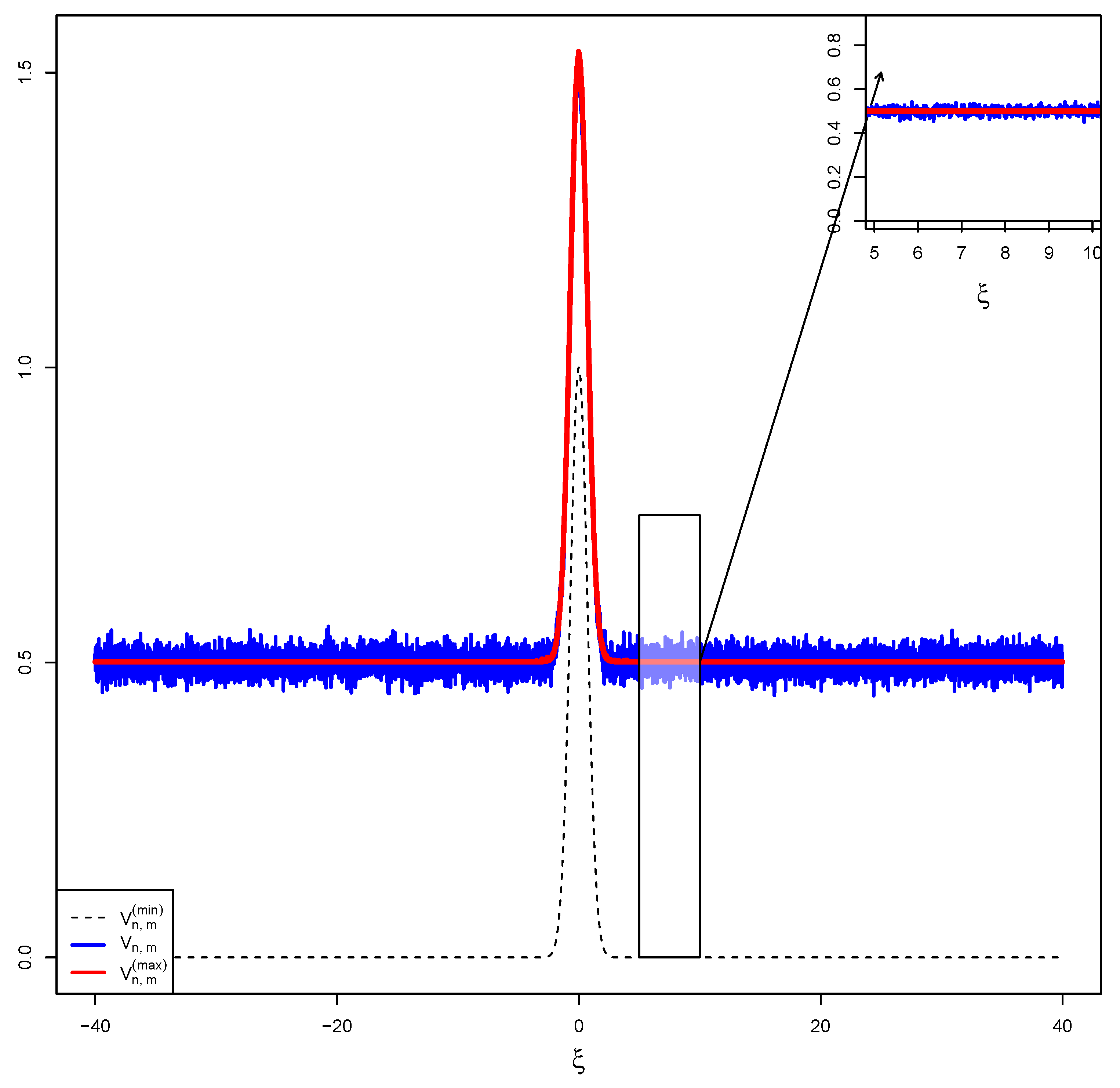
(1) We observe that V n , m ( ξ ) depends on the knowledge of V ( y i ) , which is not known in general. However, we observe that V n , m ( y j ) given in Equation (7) has minimum V n , m m i n ( y j ) = S ( y j ) and a maximum of V n , m m a x ( y j ) = 1 n + S ( y j ) because 1 m i = 1 m I [ u i , ) ( V ( y j ) ) has minimum 0 and maximum 1. This also means that although we may not know exactly the value of V n , m ( y j ) , we can estimate it to be between S ( y j ) and 1 n + S ( y j ) . We can therefore select V ( y i ) between S ( y j ) and 1 n + S ( y j ) for j = 1 , 2 , , n and the estimate of the nontrivial solution will exist in a small interval of length (bandwidth) 1 n . Hence, if the domain Ω is very dense in points y i ’s, then the nontrivial solution will be a small perturbation of the initial external input, and, if the domain is sparse, then perturbation will be greater. Henceforth, for simplicity sake, we assume that V ( y j ) U n i f S ( y j ) , 1 n + S ( y j ) . (2) Another observation is that S depends on the position of the neuron ξ in a single-layer system; however, in a multiple-layer system, it would be reasonable to think of S as depending on both the layer k and the position of the neuron on the layer, that is, S ( V k ( ξ , t ) ) .

3. Computational Algorithm

In this section, we have the setting of Theorem 1. From Remark 1, we can use the following algorithm to estimate V ( ξ ) :
  • Step 1: Select positive integers n and m.
    Here, the experimenter should choose the values of m , n relative to how much computational capabilities ones has, knowing that very large values can lead to a significant slowdown of convergence.
  • Step 2: Select y 1 , y 2 , , y n from the distribution f ( y | ξ ) .
    Knowing that f ( y | ξ ) = K ( ξ , y ) is a known probability distribution (Gaussian, Laplace, or tangent hyperbolic, see the section below), this should be achievable with relative ease from any software.
  • Step 3: Select u 1 , u 2 , , u m from the distribution of g ( u ) of U associated with G.
    As in the previous step, sampling from a known probability distribution g ( u ) should be achievable. However, if G is not given as bounded function between 0, and 1, we can still truncate it adequately to obtain a probability distribution (see Section 4.1).
  • Step 4: For j = 1 , , n , select V ( y j ) from a uniform distribution U n i f S ( y j ) , 1 n + S ( y j ) .
    This step assumes that we have an external stimulus S arriving on the neuron at position ξ given as a function of ξ .
  • Step 5: For given ξ Ω , evaluate V n , n ( ξ ) : = 1 n m j = 1 n i = 1 m I [ u i , ) ( V ( y j ) ) + S ( ξ ) .
    In this final step, one can choose different values of ξ to plot the estimator in the space Ω .
We use Step 4 only to evaluate V n , m m a x ( ξ ) . From the above algorithm, it is clear that the activation function V ( ξ ) of the neuron at position ξ is the sum of the average of activations of neurons at position y i and the external stimulus arriving at ξ . Thus, essentially, the function V ( ξ ) is a perturbation of the function S ( ξ ) by the quantity 1 n m j = 1 n i = 1 m I [ u i , ) ( V ( y i ) ) that depends on ξ and possibly of parameters of the distribution of random variables U and Y. These parameters play the role of smoothing to compensate from the noise created by small values of n , m (see Section 5).

4. Technical Considerations

In this section, we discuss the choices for the pulse emission rate function G and the connection intensity K ( x , y ) .

4.1. Pulse Emission Rate Function

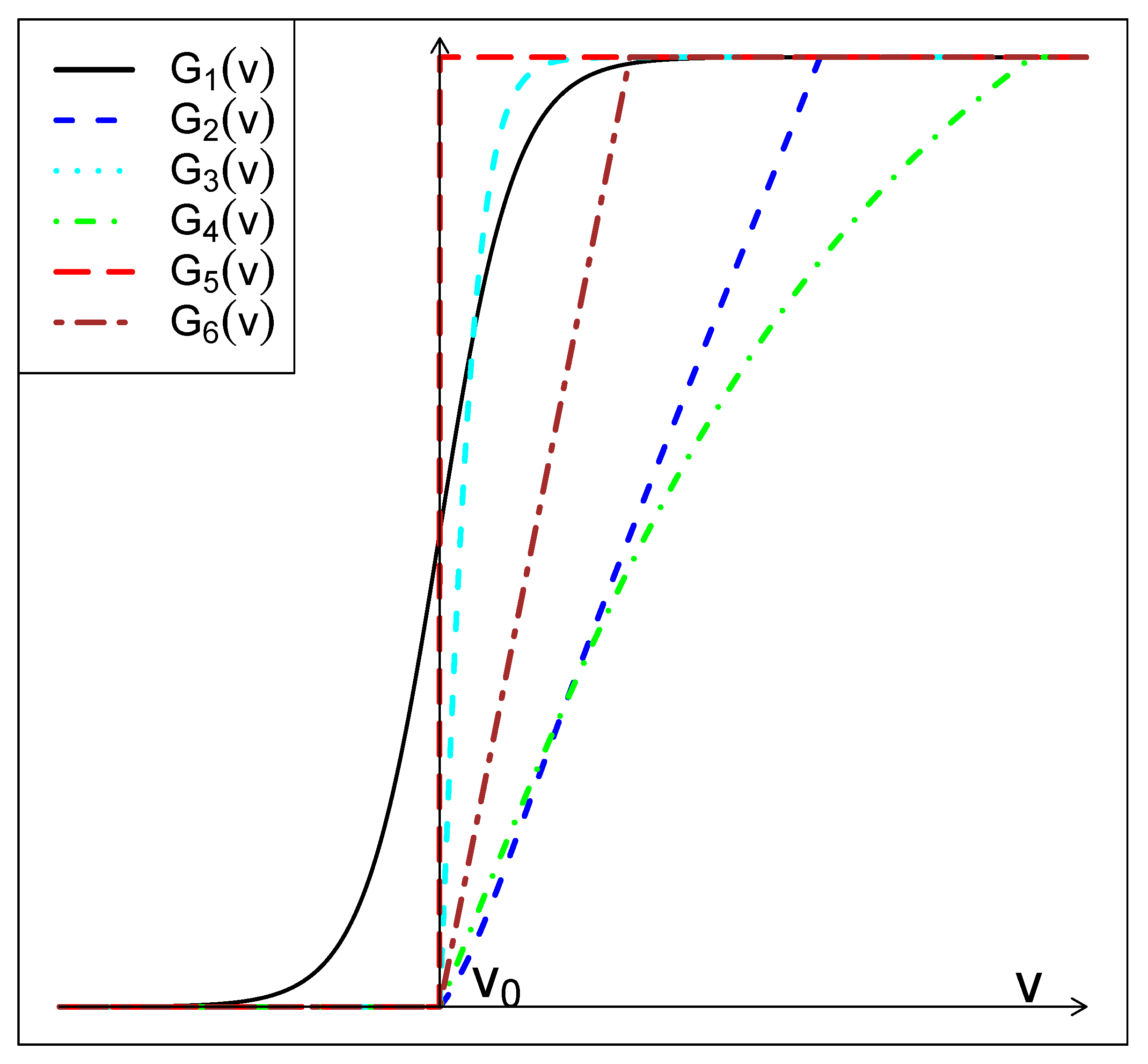
We note that Amari considered the dynamic of neural fields with pulse emission function G defined as the sigmoid function. However, the equation still has nontrivial stationary solution even if G is not the sigmoid. In fact, there is a large class of nonlinear functions G for which this is true (see Figure 2 and Table 1 below). For example, the following functions, often used in for training algorithm in artificial neural networks, have been adequately truncated for our purposes. Here, θ is a positive real number.
Remark 2.
  • (1) We observe that the choice of the sigmoid activation function G 1 ( v ) = ( 1 + e θ ( v v 0 ) ) 1 is widely preferred in the literature for its bounded nature, without condition.
  • (2) Another reason is the fact that it is also suitable when the V n ( i ) s are binary, that is, they may take the value 0 or 1, where 0 represents a non-active neuron at time n and 1 represents an active neuron at time n. In this case, G 1 W i 0 + j = 1 N W i j V n ( i ) + η n ( i ) = P r V n + 1 ( i ) = 1 would represent the probability that there is an activity on neuron at position ξ i at time n + 1 .
  • (3) A third reason, which is important in our situation, is that it has an inverse that can be written in close form, unlike many other activation functions sometime used in the artificial neural networks (see, e.g., [21]) making it easy to generate random numbers from. The other functions would require the use of numerical inversion methods such as the bisection method, the secant method, or the Newton–Raphson method, all of which are computationally intensive (see, e.g., Chapter 4 in [22]).

4.2. Connection Intensity Function

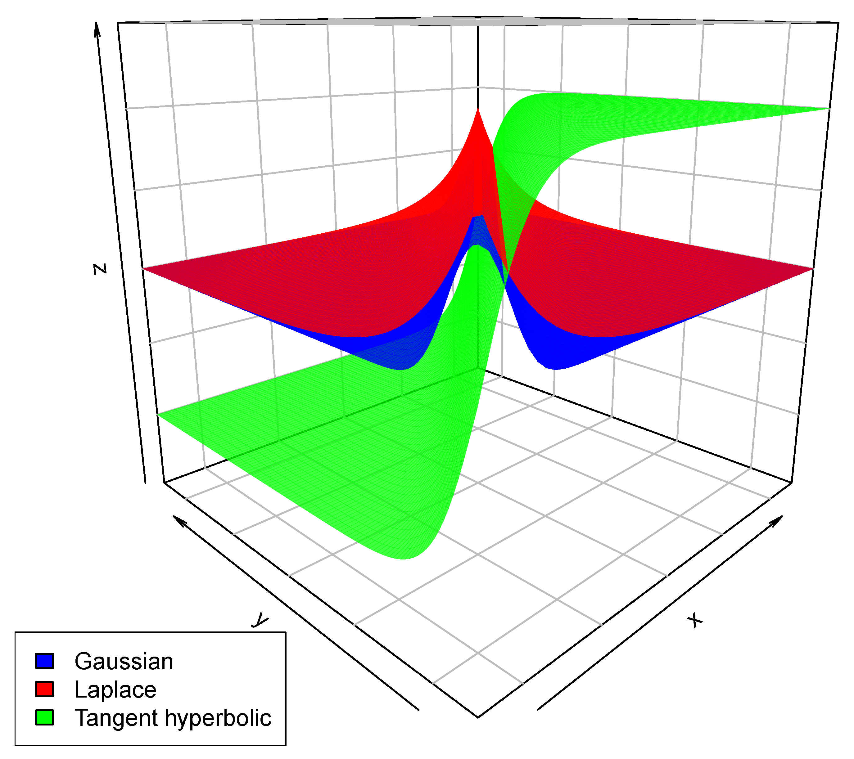
There are various connection intensities functions (or kernel) that one can choose from. These include the Gaussian kernel K ( x , y ) = 1 σ 2 π e 1 2 σ 2 x y 2 introduced above. One could also consider the Laplacian kernel defined as K ( x , y ) = 1 2 σ e 1 σ x y or the hyperbolic tangent kernel K ( x , y ) = tanh ( x y ) , see Figure 3 below for an illustration.

5. Simulations

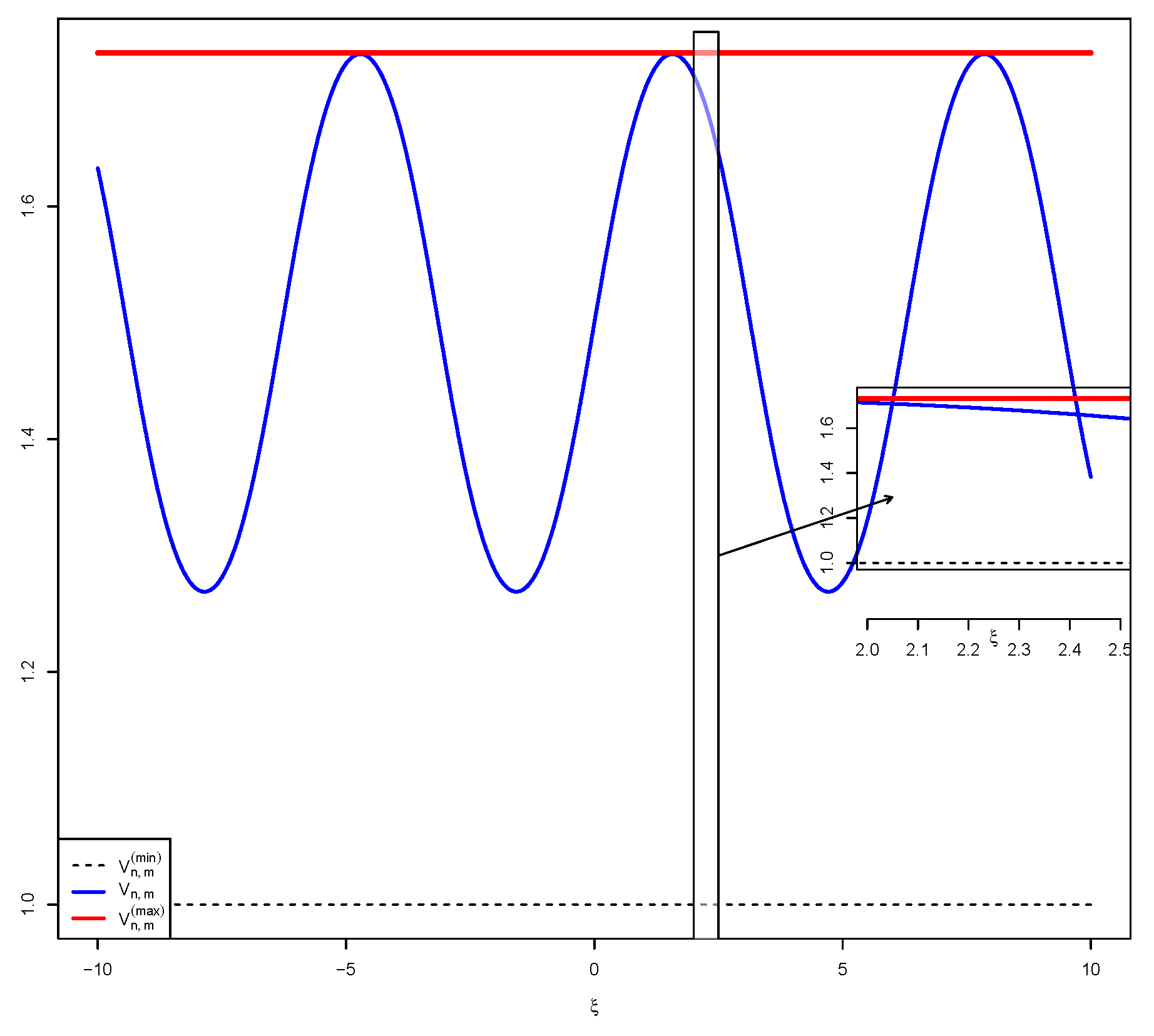
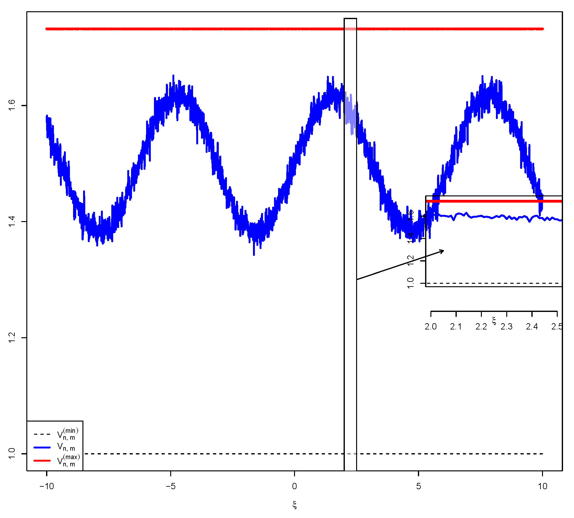
In each of the simulations below, we used the function V ( ξ ) = sin ( ξ ) as if it were the true solution, just to evaluate V ( y j ) for j = 1 , 2 , , n . Using the algorithm above, we then compare the estimates of V ( ξ ) obtained using our estimator V with V unknown (red curves) and V known (blue curves), using various kernel functions K ( x , y ) and various external stimulus functions S ( x ) . In all simulations below, we selected n = m = 100 . We used Gaussian, Laplacian, and hyperbolic tangent kernels with a sigmoid function G. The value of σ was set as 1 for the Gaussian and Laplacian kernels.

5.1. Simulation 1: Constant External Stimulus

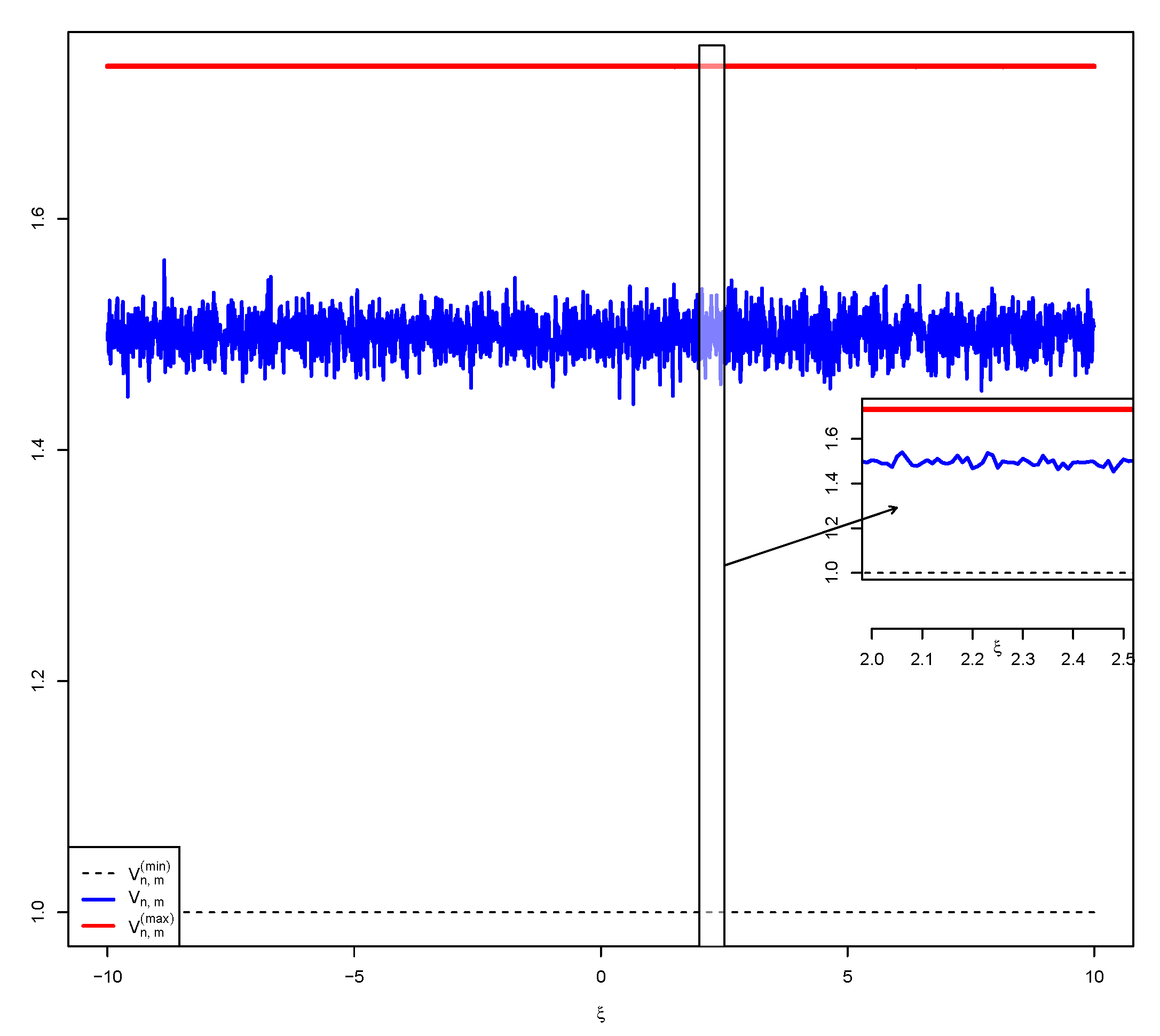
In this simulation, we illustrate the algorithm above by selection a constant intensity of external stimulus arriving at at point ξ . To check if the algorithm is correct, we select S ( ξ ) 1 , with true function V ( ξ ) = sin ( ξ ) (see Figure 4, Figure 5 and Figure 6).

5.2. Simulation 2: Logarithm External Stimulus

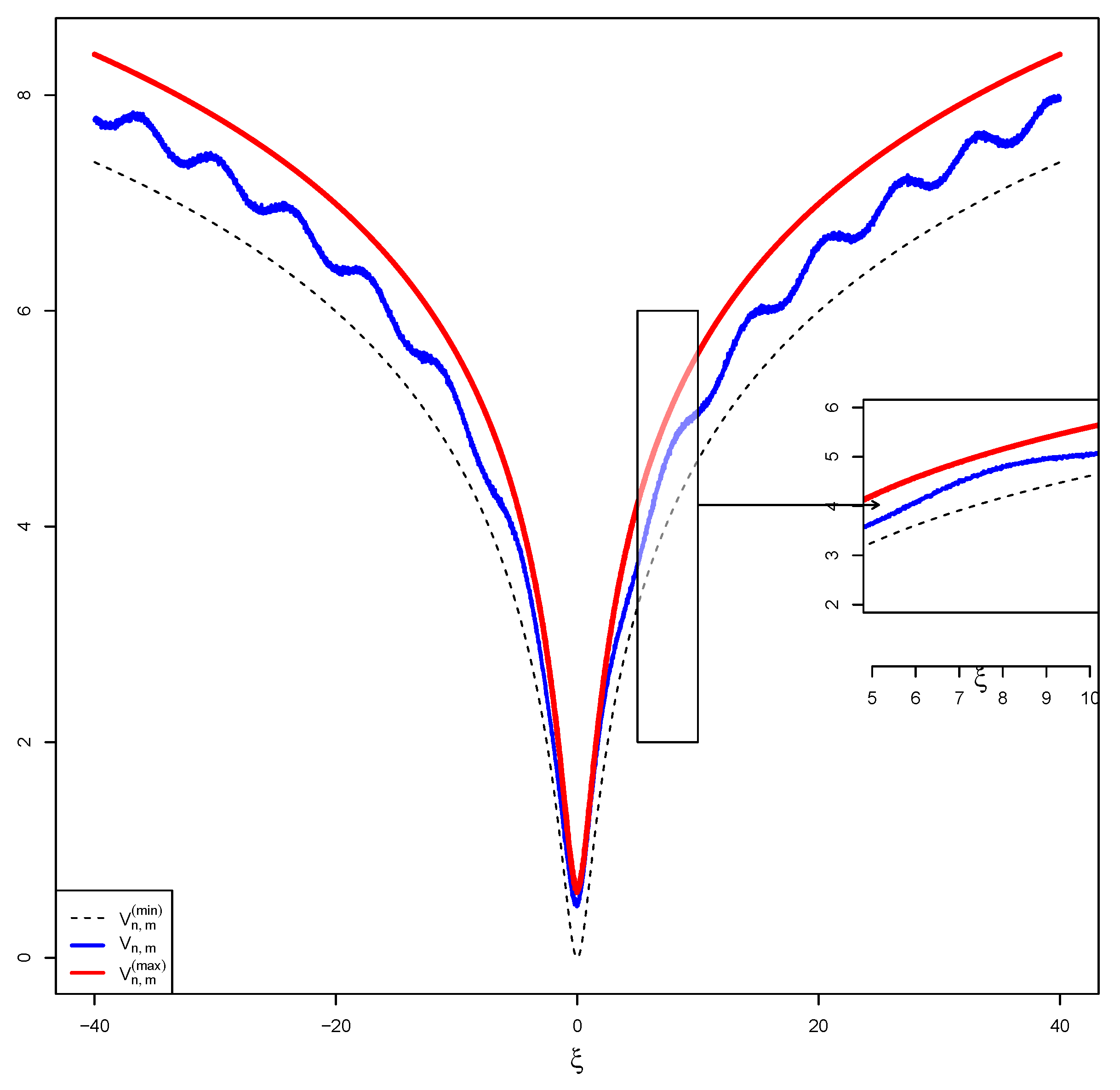
In this simulation, we illustrate the algorithm above by selection a constant intensity of external stimulus arriving at at point ξ . To check if the algorithm is correct, we select S ( ξ ) = ln ( 1 + ξ 2 ) , with true function V ( ξ ) = sin ( ξ ) (see Figure 7, Figure 8 and Figure 9).

5.3. Simulation 3: Exponentially Decaying External Stimulus

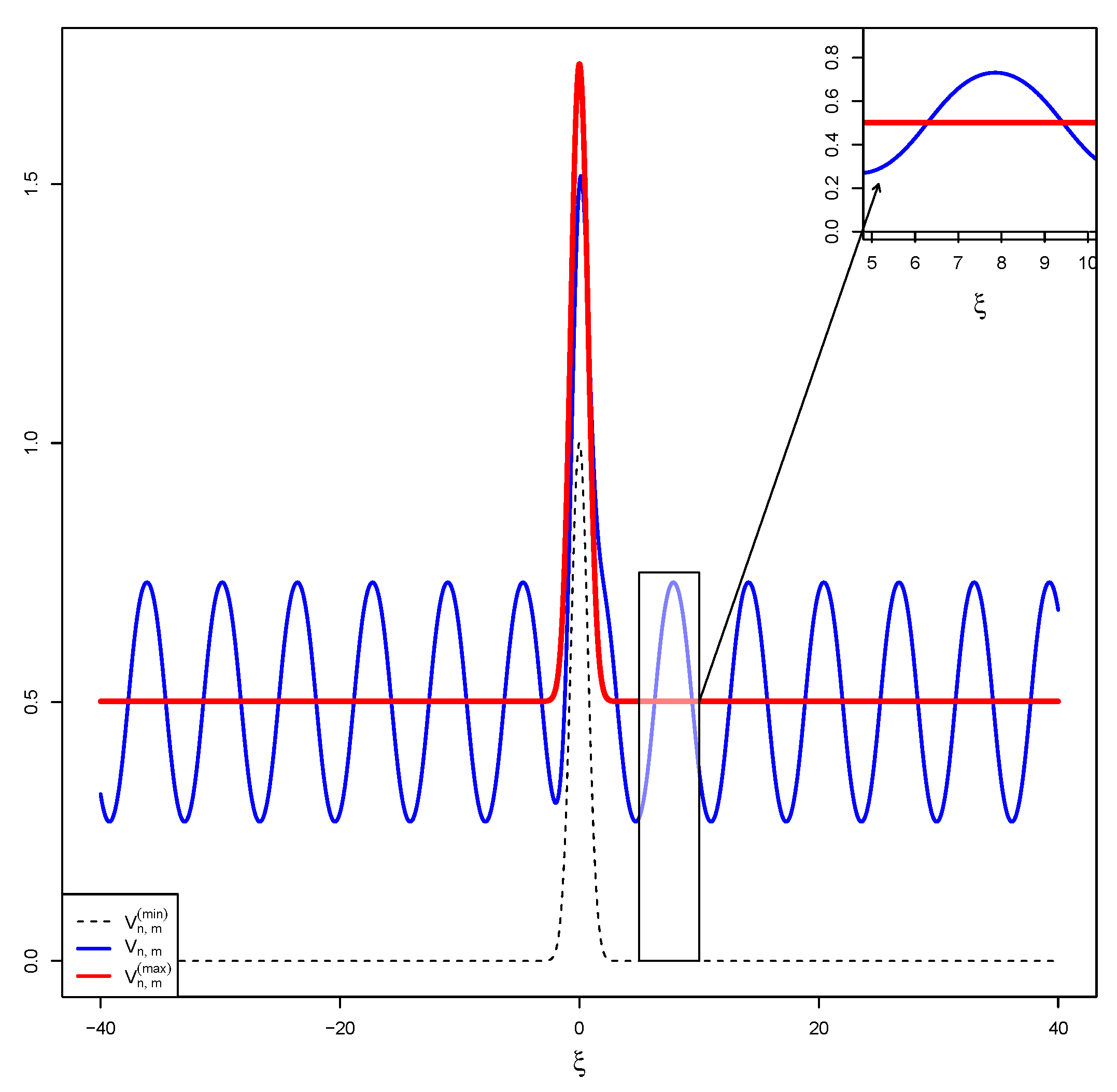
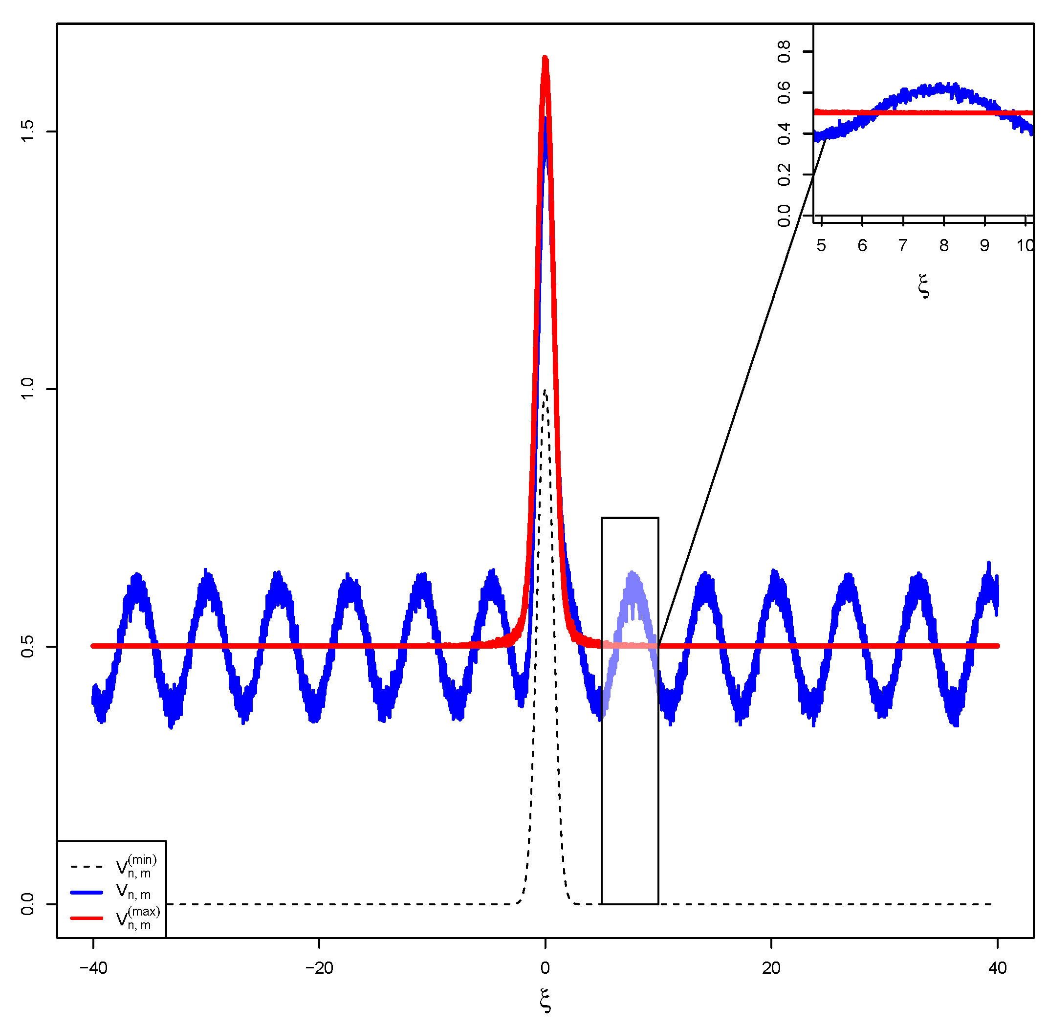
In this simulation, we illustrate the algorithm above by selection an intensity of external stimulus arriving at at point ξ as S ( ξ ) = e ξ 2 , with true function V ( ξ ) = sin ( ξ ) (see Figure 10, Figure 11 and Figure 12).

5.4. Simulation 4: Mexican Hat True Function

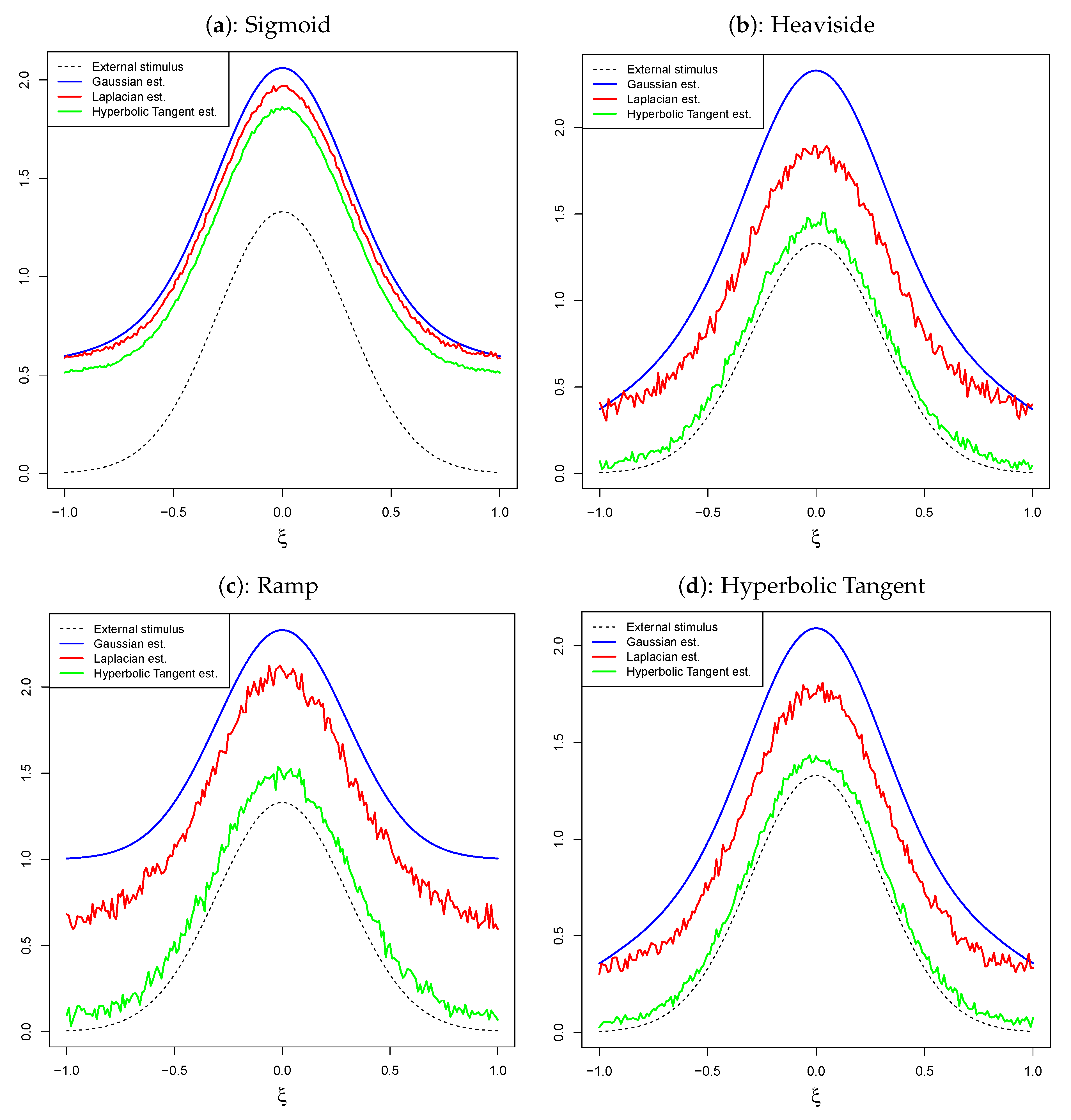
In [12], the authors used a Gaussian kernel to obtain an estimate of the nontrivial solution that had the form of a Mexican hat function in the space Ω . Our method differs from theirs in two aspects: First, they assumed that K ( x , y ) = V 0 ( x ) · V 0 ( y ) where V 0 ( x ) = Ω K ( x , y ) G ( V 0 ( y ) ) d y which implies that 1 = Ω V 0 ( y ) G ( V 0 ( y ) ) d y . This would restrict us to only independent random variables X and Y with marginals V 0 ( x ) and V 0 ( y ) . We do not make such an assumption because there are many kernels (bivariate functions) that cannot be factored as the product of two marginals. Second, we do not make the assumption that G ( V ( y ) ) has power series about certain state V ( y ) ¯ , so that G ( V ( y ) ) = n = 0 G ( n ) ( y ) n ! V ( y ) V ( y ) ¯ n . This assumption would obviously fail for the Heaviside and Ramp functions. The main reason for the difference is that they were interested in second-order synaptic dynamics, which is not the case here. In this section, we show that our method still yields a comparable estimate even without these assumptions. Indeed, in [12], the authors showed that the true solution obtained with a Gaussian kernel in the space has the form of a Mexican hat function. In this simulation, we use our estimator to verify this fact, that is, we set our external stimulus as a Gaussian distribution with mean zero and standard deviation 0.03 as in their case and compare the estimates obtained from the use of a Gaussian, Laplacian, and hyperbolic tangent kernels (see Figure 13).

5.5. Discussion

(1) The conclusion we can draw from the first simulation is that Gaussian and Laplacian kernels both fare well when the external input is constant. The latter produces noisier outputs at low resolution values n , m and becomes smother at high resolution values n , m .
(2) The major takeaway from the second and third simulations is that the external stimulus can have a significant effect on the estimator, especially near boundary points where there is a significant frequency change between the true value and the external stimulus. In reality, in practical applications, the true value is not known; therefore, a careful choice on the external input is needed if one would like to obtain accurate estimations.
(3) The fourth simulation shows that estimates obtained using a Gaussian kernel are smoother. As for the pulse rate function G, the sigmoid function G 1 fares much better for all three kernels used in comparison to other functions.
(4) Ultimately, the point of the first three simulations is the hope to extend this type of estimator beyond solutions of DNF. In fact, Equation (1) can be considered a linear Boltzmann equation with stochastic kernel if, instead of thinking of ξ as the position of a neuron, we think of it as the velocity of a particle and V ( x , t ) as the velocity distribution overtime. In this case, nontrivial solutions are now solutions of the nonlinear Markov operator P g ( v ( ξ ) ) = v ( ξ ) where P g ( v ( ξ ) ) : = Ω K ( ξ , y ) g ( v ( y ) ) d y , which by the Hille–Yosida theorem exist. The proposed estimator provides in a sense another way of thinking about this problem using successive approximations (see [23]).
(5) A drawback of the estimator is that it depends on a great first guest of the solutions at points y i Ω . However, if enough of these points are selected, one stands a great chance of obtaining a good approximation.
(6) An advantage of this estimator is that, locally, it is a great point estimator of the value of V ( ξ ) for a given ξ Ω , and given y 1 , y 2 , , y n Ω . As mentioned in Section 3, although we may not know the values of V ( y i ) , i = 1 , , n needed to evaluate V ( ξ ) , one way to go around the issue is to select them uniformly from a small interval of length 1 n .
(7) We observe that the computational aspect of our algorithm depends on Monte Carlo Simulations. This is not the only way of efficiently achieve this. One may also choose to achieve this using methods such as sparse grids and Bayesian Monte Carlo with appropriate priors on the parameters (see, e.g., [24,25,26,27,28]).
(8) One other possible use of this estimator is that it can help initialize a RNN algorithm or help find the phase space diagram in a discrete dynamical system with two different layers.

6. Conclusions

In this paper, we propose an estimator for nontrivial solutions of dynamic neural fields. The proposed estimator is shown to be consistent. Moreover, the proposed estimator exists within a small interval depending on the number of points selected in the domain Ω where these nontrivial solutions are defined.
The choice of the kernel, as in previous studies, is shown to be crucial in determining the accuracy of the estimates.
We also show that Gaussian kernels provide the best balance among accuracy, smoothness, and the number of points used. In the space domain, the estimates obtained are visually similar to those obtained using, for instance, Lotka–Volterra series, as in [12]. The proposed estimator has the advantage that it is simple to implement and may serve as initial guess or initialization when for example using a recurrent neural networks to find nontrivial solutions in the time and space domain. This is particularly important in robotics and to a certain extent in neuroinformatics because it could potentially help with accuracy of movements of robots.
In this paper, we also show how the DNF can be extended to functional and complex analysis, which could further extend theoretical properties of DNFs using techniques from these areas. The proposed estimator in this paper can be used to initialize a discrete dynamical system associated with the DNF.
The present work could be useful for new insights into the connection between DNF and dynamical systems and overall contribute to the literature in these areas and in computational neuroscience.

Funding

This research received no external funding.

Data Availability Statement

The data presented in this study are available on request from the corresponding author. The data are not publicly available due to their randomly generated nature from known distributions.

Acknowledgments

The author thank Corine M. Kwessi for the administrative and technical support that helped conduct this study to its completion. The author would also like to thank the referees for careful reading and useful comments that helped to improve the paper.

Conflicts of Interest

The author declares no conflict of interest.

References

  1. Beurle, R.L. Properties of a mass of cells capable of regenerating pulses. Philos. Trans. R. Soc. Lond. B 1956, 240, 55–94. [Google Scholar]
  2. Wilson, H.R.; Cowan, J.D. Excitatory and inhibitory interactions in localized populations ofmodel neurons. Biophys. J. 1972, 12, 1–24. [Google Scholar] [CrossRef] [Green Version]
  3. Amari, S.I. Dynamics of pattern formation in lateral-inhibition type neural fields. Biol. Cybern. 1977, 27, 77–87. [Google Scholar] [CrossRef] [PubMed]
  4. Nunez, P.L.N.; Srinivasan, R. Electric Fields of the Brain: The Neurophysics of EEG, 2nd ed.; Oxford University Press: Oxford, UK, 2006. [Google Scholar]
  5. Camperi, M.; Wang, X.J. A model of visuospatial short-term memory in prefrontal cortex: Recurrent network and cellular bistability. J. Comp. Neurosci. 1998, 4, 383–405. [Google Scholar] [CrossRef] [PubMed]
  6. Ermentrout, G.B.; Cowan, J.D. A mathematical theory of visual hallucination patterns. Biol. Cybern. 1979, 34, 137–150. [Google Scholar] [CrossRef] [PubMed]
  7. Tass, P. Cortical pattern formation during visual hallucinations. J. Biol. Phys. 1995, 21, 177–210. [Google Scholar] [CrossRef]
  8. Bicho, E.; Mallet, P.; Schöner, G. Target representation on an autonomous vehicle with low-levelsensors. Int. J. Robot. Res. 2000, 19, 424–447. [Google Scholar] [CrossRef]
  9. Erlhangen, W.; Bicho, E. The dynamics neural field approach to cognitive robotics. J. Neural Eng. 2006, 3, R36–R54. [Google Scholar] [CrossRef] [PubMed]
  10. Erlhangen, W.; Schöner, G. Dynamic field theory of movement preparation. Psychol. Rev. 2001, 109, 545–572. [Google Scholar] [CrossRef] [PubMed] [Green Version]
  11. Bicho, E.; Louro, L.; Erlhangen, W. Integrating verbal and non-verbal communication in adynamic neural field for human-robot interaction. Front. Neurorobot. 2010, 4, 1–13. [Google Scholar]
  12. Beim, P.G.; Hutt, A. Attractor and saddle node dynamics in heterogeneous neural fields. EPJ Nonlinear Biomed. Phys. EDP Sci. 2014, 2. [Google Scholar] [CrossRef]
  13. Hammerstein, A. Nichtlineare Integralgleichungen nebst Anwendungen. Acta Math. 1930, 54, 117–176. [Google Scholar] [CrossRef]
  14. Djitte, N.; Sene, M. An Iterative Algorithm for Approximating Solutions of Hammerstein IntegralEquations. Numer. Funct. Anal. Optim. 2013, 34, 1299–1316. [Google Scholar] [CrossRef]
  15. Kwessi, E.; Elaydi, S.; Dennis, B.; Livadiotis, G. Nearly exact discretization of single species population models. Nat. Resour. Model. 2018. [Google Scholar] [CrossRef]
  16. Elman, J.L. Finding Structure in time. Cogn. Sci. 1990, 14, 179–211. [Google Scholar] [CrossRef]
  17. Williams, R.J.; Zipser, D. A learning algorithm for continually running fully recurrent neural networks. Neural Comput. 1990, 1, 256–263. [Google Scholar] [CrossRef]
  18. Durstewitz, D. Advanced Data Analysis in Neuroscience; Bernstein Series in Computational Neuroscience; Springer: Cham, Switzerland, 2017. [Google Scholar]
  19. Green, R.E.; Krantz, S.G. Function Theory of One Complex Variable; Pure and Applied Mathematics (New York); John Wiley & Sons, Inc.: New York, NY, USA, 1997. [Google Scholar]
  20. Rudin, W. Real and Complex Analysis; McGraw-Hill: New York, NY, USA, 1987. [Google Scholar]
  21. Kwessi, E.; Edwards, L. Artificial neural networks with a signed-rank objective function and applications. Commun. Stat. Simul. Comput. 2020. [Google Scholar] [CrossRef]
  22. Devroye, L. Complexity questions in non-uniform random variate generation. In Proceedings of COMPSTAT’2010; Physica-Verlag/Springer: Heidelberg, Germany, 2010; pp. 3–18. [Google Scholar]
  23. Lasota, A.; Mackey, M.C. Chaos, Fractals, and Noise, 2nd ed.; Applied Mathematical Sciences; Springer: New York, NY, USA, 1994; Volume 97. [Google Scholar]
  24. Rasmussen, C.E.; Ghahramani, Z. Bayesian Monte Carlo. In Proceedings of the 15th International Conference on Neural Information Processing Systems, Vancouver, BC, Canada, 9–14 December 2002; pp. 505–512. [Google Scholar]
  25. Deisenroth, M.P.; Huber, M.F.; Henebeck, U.D. Analytic Moment-based Gaussian Process Filtering. In Proceedings of the 26th International Conference on Machine Learning (ICML), Montreal, QC, Canada, 14–18 June 2009. [Google Scholar]
  26. Gerstner, T.; Griebel, M. Numerical integration using sparse grids. Numer. Algorithms 1998, 18, 209. [Google Scholar] [CrossRef]
  27. Xu, Z.; Liao, Q. Gaussian Process Based Expected Information Gain Computation for Bayesian Optimal Design. Entropy 2020, 22, 258. [Google Scholar] [CrossRef] [PubMed] [Green Version]
  28. Movaghar, M.; Mohammadzadeh, S. Bayesian Monte Carlo approach for developing stochastic railway track degradation model using expert-based priors. Struct. Infrastruct. Eng. 2020, 1–22. [Google Scholar] [CrossRef]
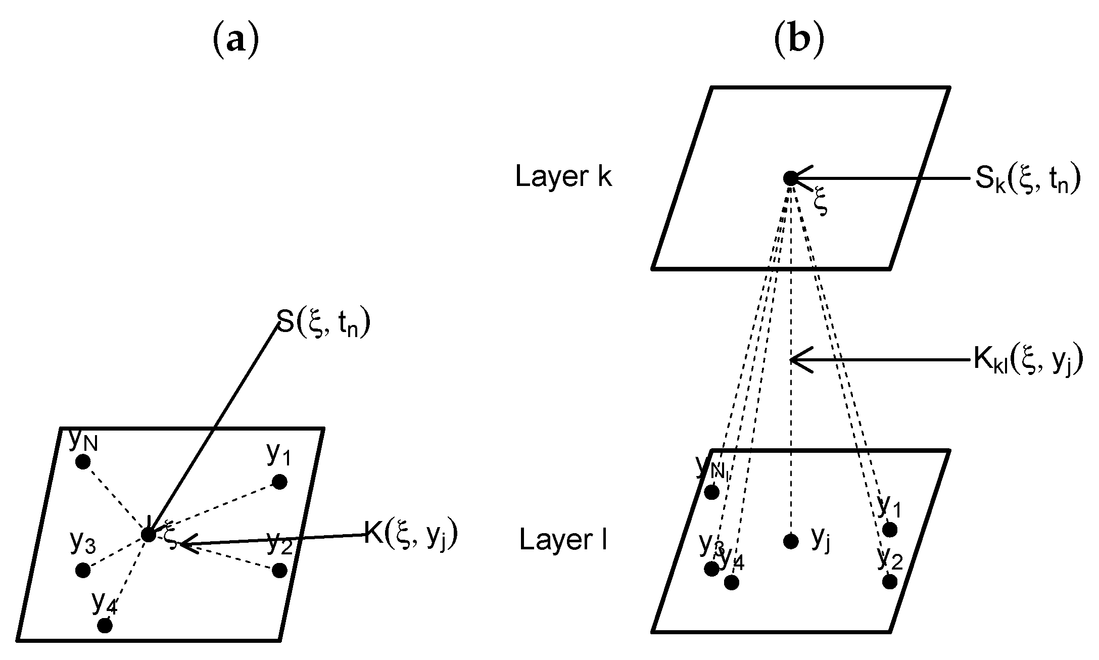
Figure 1. Illustration of the DNF for: single layer (a); and multiple layers (b).
Stats 04 00010 g001
Figure 2. Five different activation functions.
Stats 04 00010 g002
Figure 3. Illustration of Gaussian, Laplacian, and hyperbolic tangent kernels.
Stats 04 00010 g003
Figure 4. The dotted line represents the input S ( ξ ) = 1 , which from above is similar to the V n , m m i n . The kernel is a Gaussian. The maximum estimator V n , m m i n (red) has the same patterns as the external stimulus and the estimator V n , m (blue) takes the form of the true sine function.
Stats 04 00010 g004
Figure 5. The dotted line still represents the input S ( ξ ) = 1 , which from above is similar to the V n , m m i n . The kernel is Laplacian. The maximum estimator V n , m m i n (red) has the same patterns as the external stimulus and the estimator V n , m (blue) takes the form of the true sine function, but noisier at low n , m and progressively smoother at high values of n , m .
Stats 04 00010 g005
Figure 6. The dotted line represents the input S ( ξ ) = 1 , which from above is similar to the V n , m m i n . The kernel is a Hyperbolic tangent. The maximum estimator V n , m m i n (red) has the same patterns as the external stimulus and the estimator V n , m (blue) takes the form of the initial external input, unable to replicate the form of the true since function, even at high values of n , m .
Stats 04 00010 g006
Figure 7. The dotted line represents the input S ( ξ ) = ln ( 1 + x 2 ) , which from above is similar to the V n , m m i n . The kernel is Gaussian. The maximum estimator V n , m m i n (red) has the same patterns as the external stimulus and the estimator V n , m (blue) is a distorted version of the original since function, with distortion that is increased around 0, which is caused by the presence of S ( ξ ) that is in the neighborhood of 0 dominating the sine function that we know is close to 0 in a small neighborhood of 0. However, as we get farther from zero, the influence of external stimulus wanes and the estimator starts to take the shape of the true since function.
Stats 04 00010 g007
Figure 8. In this case, we use a Laplacian Kernel and we observe a similar pattern as above. However, the estimator is much noisier. There is also a noticeable phase difference between the estimations from a Gaussian kernel and a laplacian kernel.
Stats 04 00010 g008
Figure 9. In this case, we used hyperbolic tangent kernel and clearly the sine pattern of the true function is never recovered. This suggests that the external input is overwhelming the noise, even after a close look within the interval [5.0,5.1].
Stats 04 00010 g009
Figure 10. Clearly, with this external inputs, the situation is different from the above cases. In a small neighborhood of 0, we still have the external stimulus dominating; the noise and the estimates V n , m (blue) remains between V n , m m a x and V n , m m i n . However, as we move farther away from 0, V n , m m a x takes the shape of S ( ξ ) but it oscillates between S ( x ) and V n , m . This is explained but the fact that e x p ( ξ 2 ) is traded with sin ( ξ ) due to the periodic nature of the latter. The estimator on the other hand reproduces the expected pattern is this where a Gaussian kernel is used.
Stats 04 00010 g010
Figure 11. In this case, the kernel is Laplacian and the observations are the same as above. However, we observe much more noise in the estimator, together with a phase shift.
Stats 04 00010 g011
Figure 12. In this case, the expected pattern is not reproduced due to the external stimulus dominating and the estimator serving as noise.
Stats 04 00010 g012
Figure 13. The curves are estimates of V ( ξ ) using the proposed estimator for different kernels, Gaussian (blue), Laplacian (red), and hyperbolic tangent (green) with a mean zero Gaussian external stimulus with standard deviation 0.03. Clearly, all kernels yield the expected pattern: (a) the sigmoid function G 1 ; (b) the Heaviside function G 5 ; (c) the Ramp function G 6 with θ = 3.5 ; and (d) the hyperbolic tangent inverse function G 3 .
Stats 04 00010 g013
Table 1. A list of potential pulse emission rate functions one can consider in applications.
NameFormulationConditions
Sigmoid: G 1 ( v ) = 0if v < v 0
1 1 + e θ ( v v 0 ) if v v 0
Weighted Sigmoid: G 2 ( v ) = 0if v < v 0
( v v 0 ) G 1 ( v ) if v v 0
Hyperbolic Tangent: G 3 ( v ) = 0if v < v 0
1 2 G 1 ( 2 v ) if v v 0
Tangent inverse: G 4 ( v ) = arctan ( v v 0 ) if v v 0
0if v < v 0
Heaviside: G 5 ( v ) = 0if v < v 0
1if v v 0
Ramp: G 6 ( v ) = 0if v < v 0
θ ( v v 0 ) v 0 v < v 0 + θ 1
1if v v 0 + θ 1
Publisher’s Note: MDPI stays neutral with regard to jurisdictional claims in published maps and institutional affiliations.