Local Processing of Massive Databases with R: A National Analysis of a Brazilian Social Programme

Abstract

The analysis of massive databases is a key issue for most applications today and the use of parallel computing techniques is one of the suitable approaches for that. Apache Spark is a widely employed tool within this context, aiming at processing large amounts of data in a distributed way. For the Statistics community, R is one of the preferred tools. Despite its growth in the last years, it still has limitations for processing large volumes of data in single local machines. In general, the data analysis community has difficulty to handle a massive amount of data on local machines, often requiring high-performance computing servers. One way to perform statistical analyzes over massive databases is combining both tools (Spark and R) via the sparklyr package, which allows for an R application to use Spark. This paper presents an analysis of Brazilian public data from the Bolsa Família Programme (BFP—conditional cash transfer), comprising a large data set with 1.26 billion observations. Our goal was to understand how this social program acts in different cities, as well as to identify potentially important variables reflecting its utilization rate. Statistical modeling was performed using random forest to predict the utilization rated of BFP. Variable selection was performed through a recent method based on the importance and interpretation of variables in the random forest model. Among the 89 variables initially considered, the final model presented a high predictive performance capacity with 17 selected variables, as well as indicated high importance of some variables for the observed utilization rate in income, education, job informality, and inactive youth, namely: family income, education, occupation and density of people in the homes. In this work, using a local machine, we highlighted the potential of aggregating Spark and R for analysis of a large database of 111.6 GB. This can serve as proof of concept or reference for other similar works within the Statistics community, as well as our case study can provide important evidence for further analysis of this important social support programme.

1. Introduction

The use of large databases defies the traditional computational limits of data capture, processing, analysis, and storage [1]. This kind of database has become a valuable source of information collaborating in decision-making processes, as well as in the development of products and services. Consequently, questions arose about how to store and process these large data sets and which methodologies of analysis are most suitable to be used. In this context, the term Big Data is widely used today, although there is no consensus about its definition. According to [2], the use of industrial and biomedical sensors, emails, social networks, medical images, messaging applications was driven by these changes, causing the intense generation of data and the appearance of the term Big Data. Volume (the size of the data generated), variety (different data formats), and velocity (speed in which data is generated) were some of the initial concepts used to characterize big data. However, it is important to note that large databases are not necessarily big data, since the term “big” is subject to several interpretations. In this paper, we have considered large databases as those the user are not able to handle with the resources (memory, processor, disk capacity, etc) present on the machine.

Public data can be considered large databases, mainly in its raw form, as they represent a range of observations about a given population. These data are extremely important since they represent the democratization of information in a society. In this sense, the Bolsa Família Programme (BFP) is a Brazilian direct income transfer program aimed at families in poverty or extreme poverty, with the aim of reducing vulnerability [3]. BFP is quite dynamic: families enter and leave the programme every month, according to a set of conditionalities [4]. The Brazilian government provides monthly data about roughly 15 million nominal payments.

Hummon and Fararo [5] state that science today, based on data analysis, is supported by three pillars: “theory” “empirical,” and “computation”, showing the importance of the evolution of computing with data analysis for the development of modern science. One possible way to analyze this type of data is through machine learning methods. Supervised machine learning refers to predictive algorithms, that is, they are models with a strong focus on data prediction. An advantage of these mod using the R connection API with Spark-els is that they do not need assumptions like classical statistical models [6]. One of the most used algorithms in machine learning is the Decision Tree model, which consists of predicting the response variable based on decision criteria obtained from the data itself.

In order to perform this kind of analysis over large databases, the use of parallel computing techniques has been beneficial. In general, a large amount of data is divided into smaller pieces to be processed in parallel and then regrouped into a single set. In this context, some tools have been developed over the years, including Apache Hadoop [7] and Apache Spark [8], which is a unified computing engine and set of libraries for processing parallel data in computer clusters [9]. Apache Spark is a project from the Apache Software Foundation written in Scala and providing Application Programming Interfaces (APIs) in Python, Scala, Java and, R. One way to perform statistical analyzes over massive databases is combining both tools (Spark and R) via the sparklyr package, which allows for an R application to use Spark [10].

This paper presents a methodology for analyzing large volumes of data using the sparklyr package and R on a local machine. We present a short introduction to this package and a case study using a real large database of 111.6 GB and 1.26 billion observations from the Bolsa Família Programme (BFP). Our main contribution is helping to disseminate the use of the sparkylr environment for large data cases, using the R connection API with Spark, as well as to present a practical, novel case study on conditional cash transfers supporting poor families that demonstrate the large socioeconomic difference in Brazil. Therefore, it present a new approach that differs from traditional one, since most recent works use sparklyr to deal with big volume of data [11,12].

The remaining sections of the paper are organized as follows: Section 2 presents some related work. Section 3 provides a brief description of computational environments based on Apache Hadoop and Apache Spark, as well as an introduction to the sparklyr package. In Section 4, we present an overview of the Random Forest algorithm, as well as its use for variable selection and validation. Section 5 brings the results obtained when analyzing public data from BFP. Finally, in Section 6 we discuss some contributions and future work ideas.

2. Related Work

It is very common today to find large databases in the Web with information from different areas of knowledge. For example, BitTorrent is a very popular P2P communications protocol in which people can share files [13]. In Brazil, there is a massive volume of structured, semi-structured, and non-structured public data available on government sites, so that the public administration is more open and transparent. The authors in [14] have developed a soft system methodology that transforms open government public data into open linked data, according to the objective of specific groups. In terms of the analysis of Brazilian social data, the literature usually presents studies that use grouped data or samples (e.g., [15,16,17]).

We can mention some works that used Apache Spark to perform data analysis: in [18], it was used to analyze tweets transmitted with very little latency (few seconds). In [19], Spark and Hadoop were used and compared for analyzing log files. The study concluded that Spark, due to its effective exploitation of main memory and efficiency use of optimization techniques, was faster than Hadoop. In [20], the authors have used deep learning in mobile big data analytics and discussed a scalable learning framework in Apache Spark. Apache Spark was used to apply machine learning operations to big data in [21], with a consideration that Spark can turn the preprocessing step considerably easier.

The literature still has few examples on the use of sparklyr to address big data applications. Most citations are related to commercial products/tools or specialized studies. This section briefly lists some related works making using of R and sparklyr within statistical data analysis scenarios. Gopalani [22] compared and discussed Hadoop and Spark, and analyzed performance using the k-means machine learning algorithm. Bluhm [11] illustrated the use of Spark in Econometrics. Also, Yu et al. [23] introduced GeoSpark to manipulate spatial data. In addition, Azevedo et al. [24] created a data visualization through the Shiny package in which the data processing was carried out through sparklyr. However, these computational tools are still little explored by the statistical community. Some examples of works in computational sociology are also found: ref. [25] shows how trends in the field have reshaped sociology. Humon and Fararo [26] talks about computational sociology, which consists of the analysis of empirical data, theoretical explanation and computational simulation. Salgado and Gilbert [27] expose the dialogue between social theory and computational models of social processes.

3. Computational Environment

3.1. Apache Hadoop

Apache Hadoop is an open source project from Apache Software Foundation, written in Java, and encompassing a collection of related subprojects that fit into the distributed computing infrastructure [28]. The main characteristics that made Hadoop interesting for applications in large databases are [29]:

• a permissive free software license;
• scalability, allowing execution in cluster environments with hundreds of servers;
• fault tolerance, ensuring the availability of data and execution of tasks even in the event of failures.

Basically, Hadoop has the storage of data sets by Hadoop Distributed File System (HDFS), which provides distributed storage, and a programming model by MapReduce, which subdivides the task for faster processing. The MapReduce programming model is used to process data in parallel, dividing the data into smaller fractions and distributing them to clusters. In this way, processing time is reduced. An example of this programming model can be seen at [30]. Thus, there are two main phases: Map and Reduce. A map() function receives the data and returns a key-value pair, while the reduce() function aggregates the information.

3.2. Apache Spark

Apache Spark is a unified computing engine and a set of libraries for processing parallel data in computer clusters [9]. It is also a project of the Apache Software Foundation and written in Scala language, which is more efficient because it executes the processing faster. Spark uses the DAG (Directed Acyclic Graph) execution model, which offers better flexibility and performance than MapReduce, that allows a multiple levels forming a tree structure, being more flexible and allowing features such as map, filter, union, etc [28]. Spark’s popularity has increased in recent years because it is easy to implement with existing technologies, such as HDFS and HBase data sources. Also, it includes the Spark Streaming, Spark SQL, Spark GraphX and Spark MLlib libraries, which are suitable for processing data in streaming, SQL, graphs and machine learning algorithms, respectively.

Spark presents the following abstractions [9]: DataSet, DataFrame, SQL tables and resilient distributed data sets (RDDs), which represent distributed collections of data. To perform the parallelism, the data is divided into partitions, a set of lines that are on a machine. Just as, when a transformation is made in a DataFrame, in fact it results in a set of RDD transformations, and practically all Spark code is compiled into the RDD. Two types of procedures are valid over RDDs:

• Transformations: return a new RDD, such as map, filter and coalesce;
• Actions: return a new value, such as reduce, collect and count.

RDD uses lazy evaluation, that is, an execution is started when an action function is triggered. Thus, Spark does not perform calculation until it is really needed. Also, the use of Spark becomes more accessible since its APIs facilitates data processing. Spark currently provides APIs in Python, Scala, Java and R. For more details see [31].

3.3. R and Spark with Sparkylr Package

A traditional tool that has grown significantly in recent years, becoming one of the main tools for data analysis and visualization, was the R software, which is a language and environment for statistical computing and graphics [32]. It is a free software, with simple syntax and that has a variety of packages that facilitate data analysis. However, as for the processing of large volumes of data, it has a native limitation, since in its standard version the data is read into the computer’s RAM memory. However, one way to work with large databases still in R is to increase it through the use of packages.

The sparklyr package was developed by Javier Luraschi et al. in order to link R to Apache Spark. Conforming to [33], in this way the ease of use of R is combined with the computational strength of Apache Spark, making it possible to reconcile the writing of a simple and fluid code with the processing of large databases without the need to learn new programming languages. Furthermore, it is compatible with other R packages, such as dplyr and capable of connecting to local or remote clusters, which can increase the processing power. A standard workflow in sparklyr is given by:

• Spark connection
• Data analysis
• Spark disconnect

Recently, the analysis of large volumes of data has been highlighted as regards the resolution of problems involving fraud detection, recommendation of products and services and identification of similar customers, for example. For this, it is important that the models used learn from the data and make good predictions, which is why Machine Learning algorithms have become so popular recently.

In order to introduce the usage of the sparklyr package, we display in following some basic commands in

Table 1. Basic commands in the sparklyr package.

Commands	Description
install.packages (“sparklyr”)	Install the sparklyr package from CRAN
library (“sparklyr”)	Load the package
spark_install()	Install Spark
sc <- spark_connect (master="local")	Create a local connect with R and Spark
spark_connection_is_open (sc)	Verify if the connection is available
spark_read_csv(path)	Read datasets in CSV (Comma Separated Values)
dataset %>% select (columns)	Select columns
src_tbls (sc)	Check the datasets that are in Spark
glimpse (dataset)	Check the dataset structure
spark_disconnect (sc)	Disconnect from Spark

. Furthermore, the entire code applied to perform this paper analyses is shared in the results section.

4. Performing Machine Learning with Random Forest

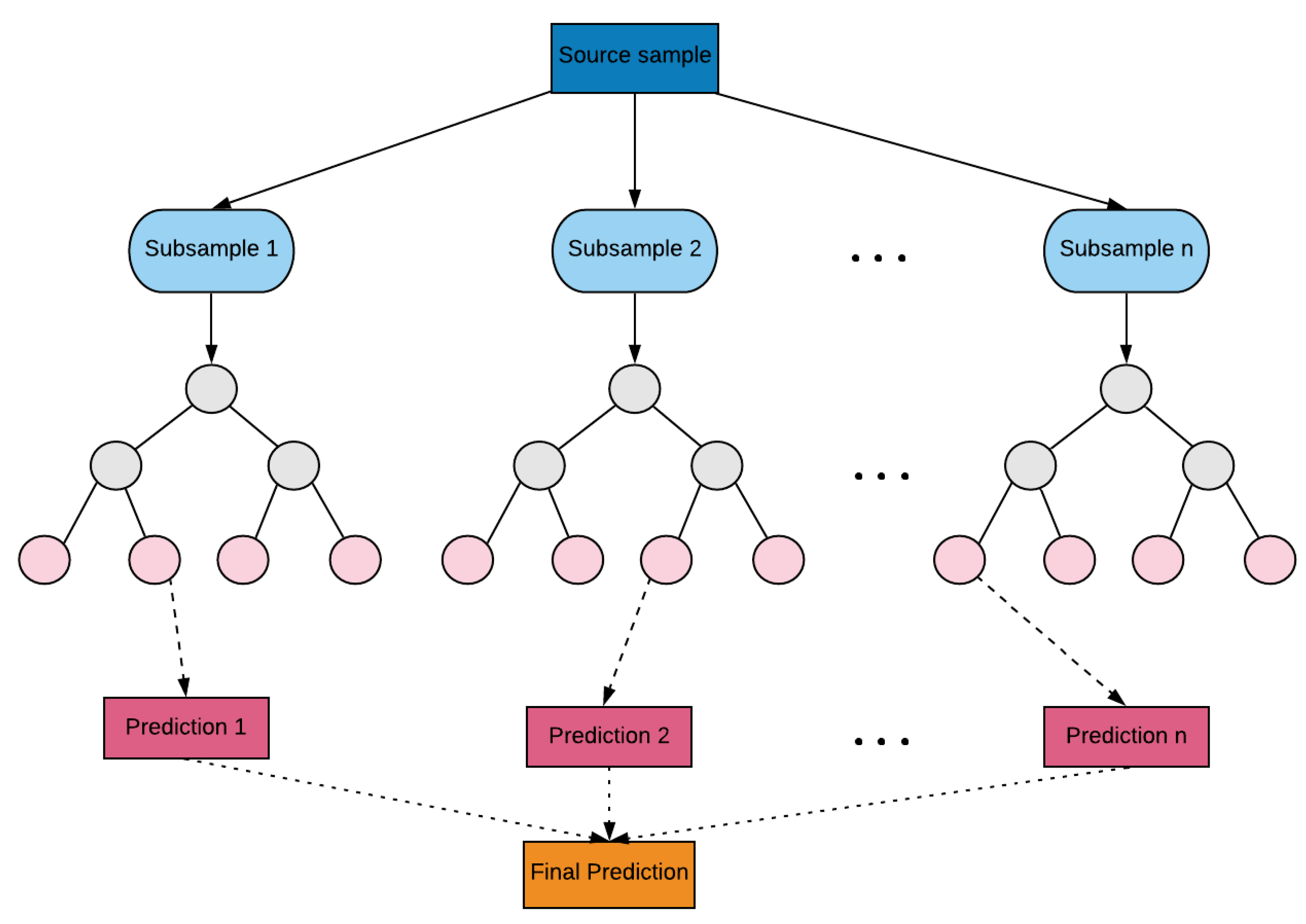
The Random Forest (RF) algorithm [34] uses the idea of combining models. This idea constitutes the ensemble methods, which combine models with the intention of balancing bias and variance. According to [35], bias refers to how well the model approaches the real relationship between variables, and variance refers to how much the model varies, depending on the sample used for training. Regarding this trade-off, the ensemble procedure is possible to reduce the variance, without increase the bias-variance [36]. Random Forest differs from other ensemble methods, like gradient boosting, due to its interpretability through the feature importance, and the independent structure of its base-learners which can provide an easy parallelization setting [34].

This methodology consists of generating multiple decision trees in parallel, where $h(\mathit{x},{\theta }_m),m=1,\cdots ,M$ where $\mathit{x}$ is an observation, such that $\mathit{x}\in {\mathbb{R}}^p$, associated with the random variable $\mathit{X}$, where p is the number of variable. The combination of all these models form “forest”. Figure 1 shows the structure of a RF.

The prediction of new observations $x^{*}$ using all the trees are given by

$$H\left({\mathit{x}}^{*}\right)=\frac{1}{T}\sum _{i=1}^T{h}_i({\mathit{x}}^{*},{\theta }_m),$$

and

$$H\left(\mathit{x}\right)=mode{\left\{h_i(\mathit{x},{\theta }_m)\right\}}_i^T,$$

respectively for regression and classification tasks, where T is the number of trees in a forest.

As a result of applying the average results of a high number of trees, the method loses the interpretation obtained with the individual decision trees [6]. Two important parameters in adjusting the RF are $ntree$ and $mtry$. The first refers to the number of trees to be built and the second the number of covariates chosen at random for each division. In general, a classification model requires $\sqrt{p}$ as the number of random selected variables for each division, where p represents the total number of covariates. For a regression model, this amount is given by $p/3$. In RF, the error estimate is obtained through the out-of-bagging (OOB) sample, which is composed by the observations that are left out of the bootstrap sample, that is, they are not used in the construction of the tree.

4.1. Selection of Variables

The procedure for selecting variables is based on the importance of the variable. According to [38], the selection of variables has two objectives: to find important variables related to the response variable (for interpretation purposes) and to find a parsimonious number of important variables (for forecasting). For this work, we are interested in the first objective.

4.2. Pseudocode

The random forest can be designed as follows:

• Let N be the total number of observations in the database and B a large number of repetitions. Sample, B times and randomly, N observations with replacement (bootstrap samples);
• Let M be the total number of covariables in the database. Select, at random and without replacement, a subset of covariates such that $m<M$ variables, for each sample previously selected. The value of m is the same always;
• Train a DT for each sample taken. Each tree will have maximum growth, therefore there is no pruning;
• Get the forecast for each of the trees;
• The final forecast is obtained by means (quantitative variables) or fashion (qualitative variables).

Just as [38], the steps for selecting variables are:

• Ordering
  • Calculate the importance of variables;
  • Discard minor variables, as the most important ones have the greatest impact;
  • Order the remaining variables in decreasing order of importance and plot them together with the corresponding standard deviation. The minimum value of the CART model forecast that fits this curve is used as a cutoff point of importance, to maintain only the K variables that exceed that point.
• Selection
  • Build nested RF models including the first k variables, starting with the model with only the most important variable, calculating the OOB error rates;
  • Select the variables involved in the model that lead to the smallest OOB error.

4.3. Validation and Evaluation Measures

In machine learning, model validation is referred to as the process to verify the suitability of the trained model in a perspective of predictive performance on new data. Refaeilzadeh et al. [39] verified that there are at least four methods of machine learning validation starting from resubstitution, hold-out, k-fold, and leave-one-out or Jackknife. In this paper we consider a repeated holdout validation, which provides a better estimate once it reduces the bias, especially compared to the standard holdout validation method [40]. This behavior is observed because instead of selecting just one sample to train a model and evaluate it, multiple samples are used, minimizing the effect of choosing a single set of observations in the simple holdout.

During the entire validation process it is important to consider some evolution measures. For a regression problem, the most used metric is the Mean Square Error (MSE), which is the average of the squared model errors. The best model is the one with the lowest MSE value. This metric is given by:

$$MSE={\displaystyle \frac{{\sum }_{i=1}^n{(y_i-\widehat{y_i})}^2}{n}}.$$

Frequently, for a binary classification problem, the metrics come from the confusion matrix, as exemplified in

Table 2. Binary confusion matrix.

Predicted value	Real Value
		Yes	No
	Yes	TP	FP
	No	FN	TN

,

Where TP represents the positive true values, TN the negative true values, FP the false positive values and FN the false negative values. In this paper, the following evaluation measures were used to quantify the performance of our binary classification model.

• Accuracy: considers the total number of correct answers in the model over the total number of observations. The best model is the one with the highest accuracy. It is defined as:

  $$ACC={\displaystyle \frac{TP+TN}{TP+TN+FP+FN}}.$$
• F1 score (F1): represents a combination of two other metrics, Recall (R) and Precision (P). The best model is the one with the highest F1 value. It is defined as:

  $$F1={\displaystyle \frac{2*P*R}{P+R}}.$$

  where $R={\displaystyle \frac{TP}{TP+FN}}$ and $P={\displaystyle \frac{TP}{TP+FP}}.$
• Matthew’s Correlation Coefficient (MCC): represents a linear qualitative correlation between prediction and real values. The best model is the one with the largest MCC. In comparison with F1-score and accuracy, the MCC produces more reliable estimations, since the other two parameters can generate overoptimistic inflated results, especially on imbalanced datasets [41]. The coefficient is defined by:

  $$MCC={\displaystyle \frac{TP\times TN-FP\times FN}{\sqrt{(TP+FP)(TP+FN)(TN+FP)(TN+FN)}}}.$$

5. Results and Data Analysis

Public data from the Bolsa Família Programme (BFP) were used to illustrate an analysis of large databases using the R software and the sparklyr package. All analyzes were performed using software R version 3.6.0 using the RStudio integrated environment [42] and performed on a personal laptop with the following configuration: Windows 10 64-bit operating system, Intel Core i3-5005U processor 2.00 GHz and 4 GB of RAM. It is worth mentioning that neither GPU nor virtual nodes were used. In fact, the Spark connection in a local mode starts with single process that runs most of the cluster components like the Spark context and a single executor [33]. Moreover, the package sparklyr version 1.0.1 and Spark version 2.4.0 were used. The main code is available at https://github.com/LED-UFBA/sparklyr_bf.

5.1. Data Description

The data used refer to the monthly payments of the BFP in the period from 2013 to 2019 and were extracted from the Brazilian Transparency Portal [43]. The downloaded files are of the CSV format and together a total size about 111.6 GB with 1.26 billion observations. The reference year and month variables were removed from the databases, as the data are in files separated by month. Thus, the considered variables are shown in

Table 3. Variables of the monthly payment bases for beneficiaries.

Variable	Description
UF	State (Federative Unit)
Code SIAFI	City code in SIAFI
Name SIAFI	City Name in SIAFI
NIS	Number of social identification
Value	Amount received by BFP

Source: adapted from the Brazilian Transparency Portal (2019) [43].

, which SIAFI corresponds to the Integrated Financial Administration System.

5.2. BFP Analysis for the Period from 2013 to 2019

The BFP analysis aims to obtain quantitative knowledge regarding the program in Brazil, aiming to know the most dependent and independent locations regarding the use of the benefit, as well as to identify the variables that are potentially important for the use of the program. For this, there is an interest in the number of beneficiaries and in the rate of use of the program. Usage rate is understood as the ratio between the total beneficiaries and the total population measured in the last 2010 Census provide by Brazilian Institute of Geography and Statistics [44]. The BFP utilization rate may be viewed as an important social indicator as well as it is related to the country’s social issues. Thus, when there is a high rate it is reflected that many people are in the poverty or extreme poverty range. The utilization rate is the ratio between the number of personal benefits and size of population in each city and for each month. Thus, the BFP utilization rate by city is the average over the observed months. The average was chosen in order to represent the general behavior of the utilization, however other statistics may be considered in future works. The understanding of the BFP utilization ratio is relevant to support Brazilians public policies, because this variable is directly associated with social problems as the unemployment and poverty. Therefore, cities with high values of this ratio can receive more social/economic assistance and directed public policies from the government, in order to improve life’s quality in those places.

First, the databases were converted from .csv to .parquet and the year and reference month variables were removed. The BFP beneficiaries were aggregated by city in order to consider the utilization rate in each of the 5.565 Brazilian cities.

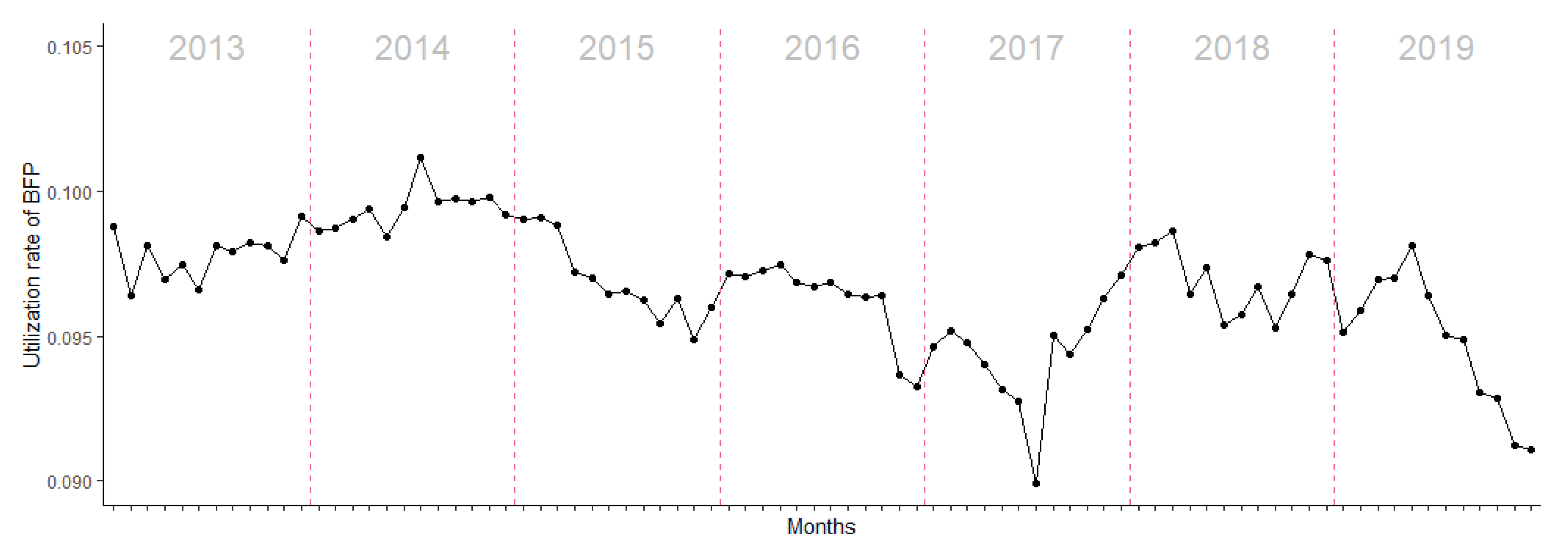
In general, performing a temporal descriptive analysis for the utilization rate of BFP (Figure 2), we can observe that utilization rate is around 10%, which means that, on average of cities, one in each ten people receives the benefit in Brazil. Also, and that the largest number of beneficiaries occurred in July 2014 and the lowest in July 2017. However, there is a decay in utilization rate after May 2019. The drop was due to government actions in 2017 and 2019, such as registration irregularities or cut of funds. Despite it being useful to consider changes over time in order to identify periods with abnormalities, Figure 2 displays the behavior of the utilization rate of BFP in Brazil over the years.

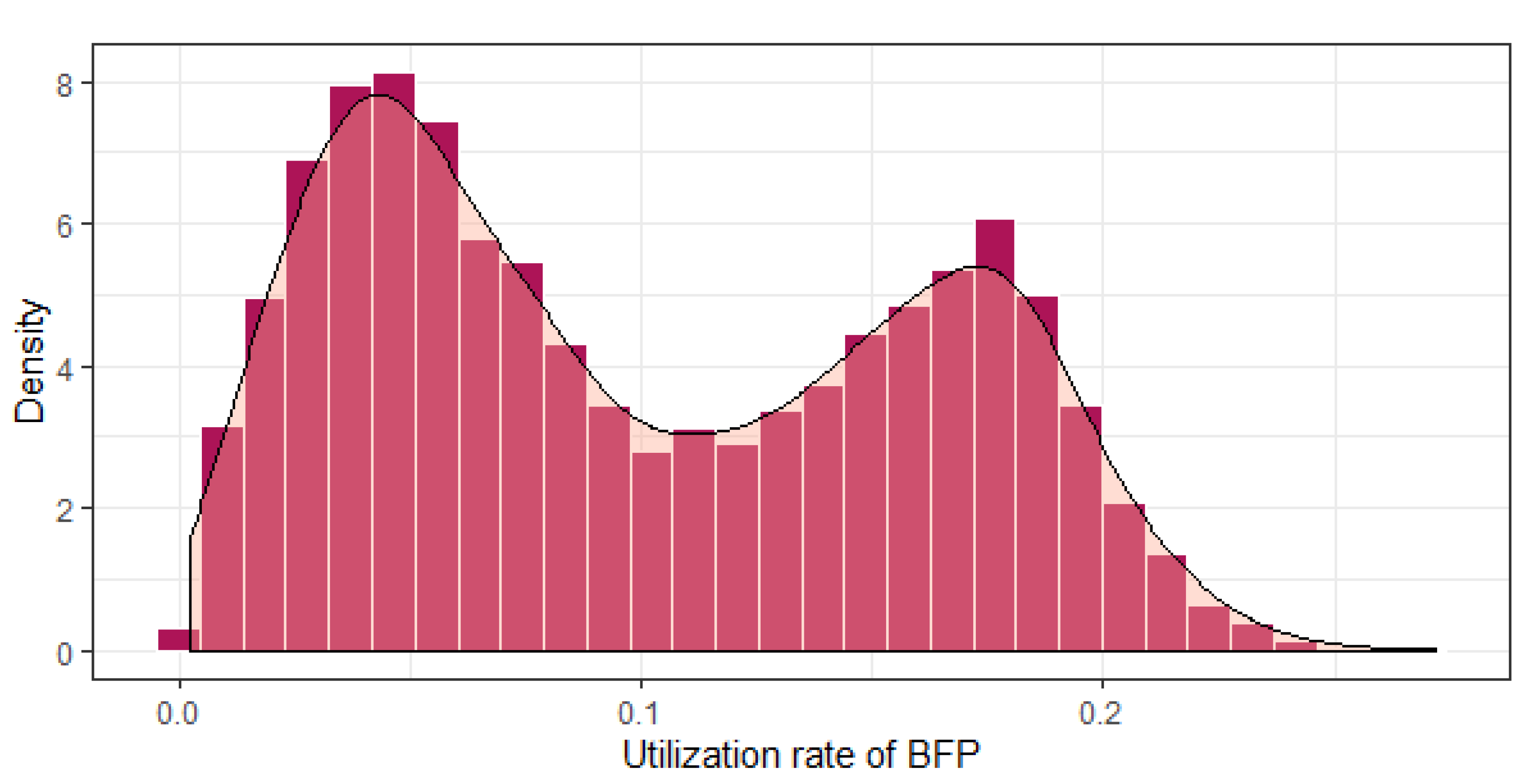
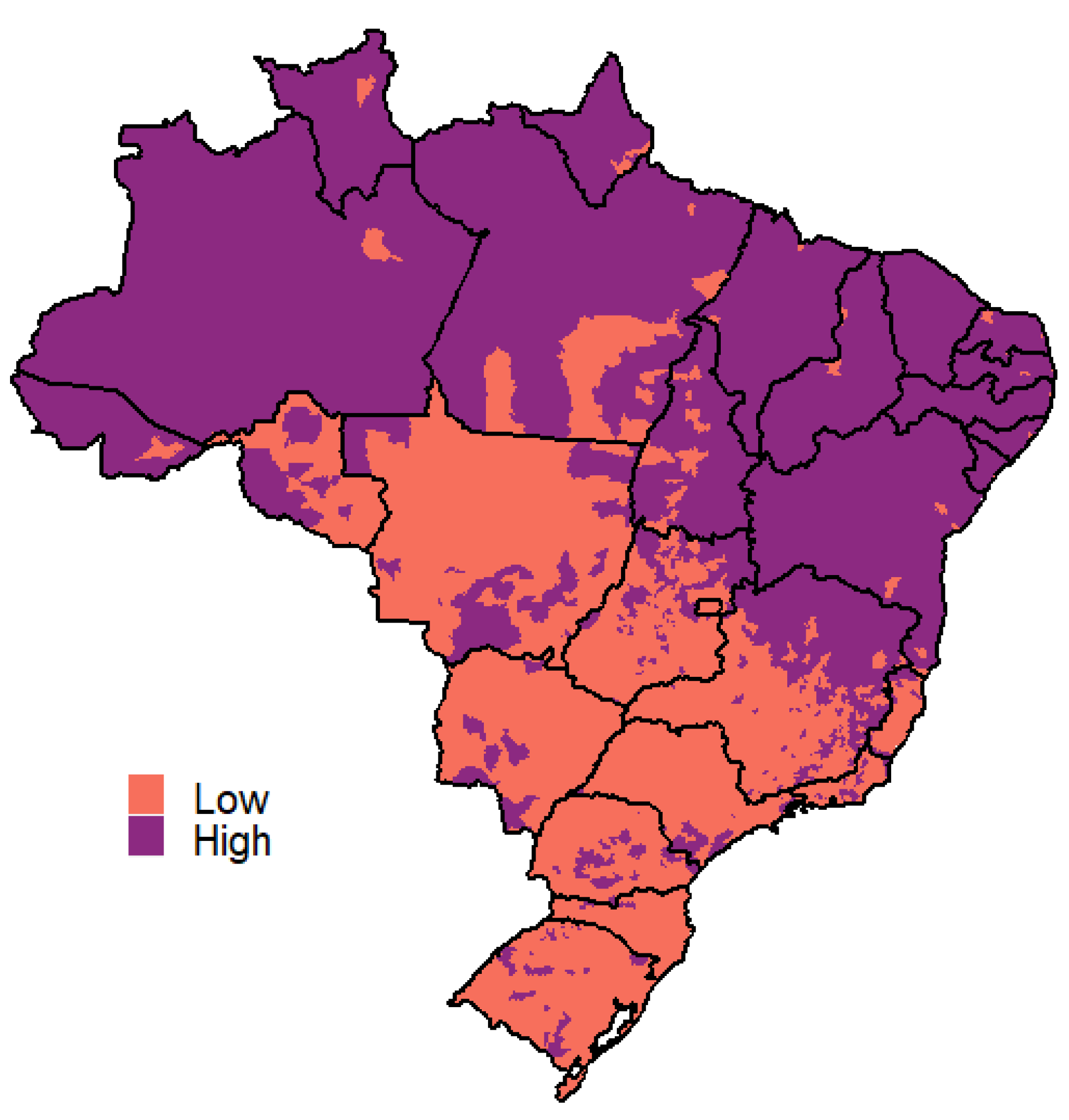
Furthermore, Figure 3 describes the distribution of the utilization rate in each city, which has a bimodal behavior that shows there are at least two kinds of cities in Brazil, stated by a low and a high utilization of BFP. In this sense, we performed a dichotomization over the mean (11%). In this sense, maps were drawn up with the average city utilization rates of the BFP, for the years studied, in a categorized way. Through Figure 4 shows that the highest rates are found predominantly in the cities from the North and Northeast regions of Brazil. Figure 5 displays the both categories for each Brazilian state. The states that have the highest utilizaiton rate is Alagoas (AL), Sergipe (SE), Piauí (PI) and Maranhão (MA). The states that have the lowest utilization rate are Santa Catarina (SC), São Paulo (SP), Rio Grande do Sul (RS) and Paraná (PR). From this outcome, is clear that BFP has different behavior in distinct cities and, between the north/northeast region with the south/southeast discrepancy is more evident. These outcomes can support specific policies from the government to improve the programme’s efficiency.

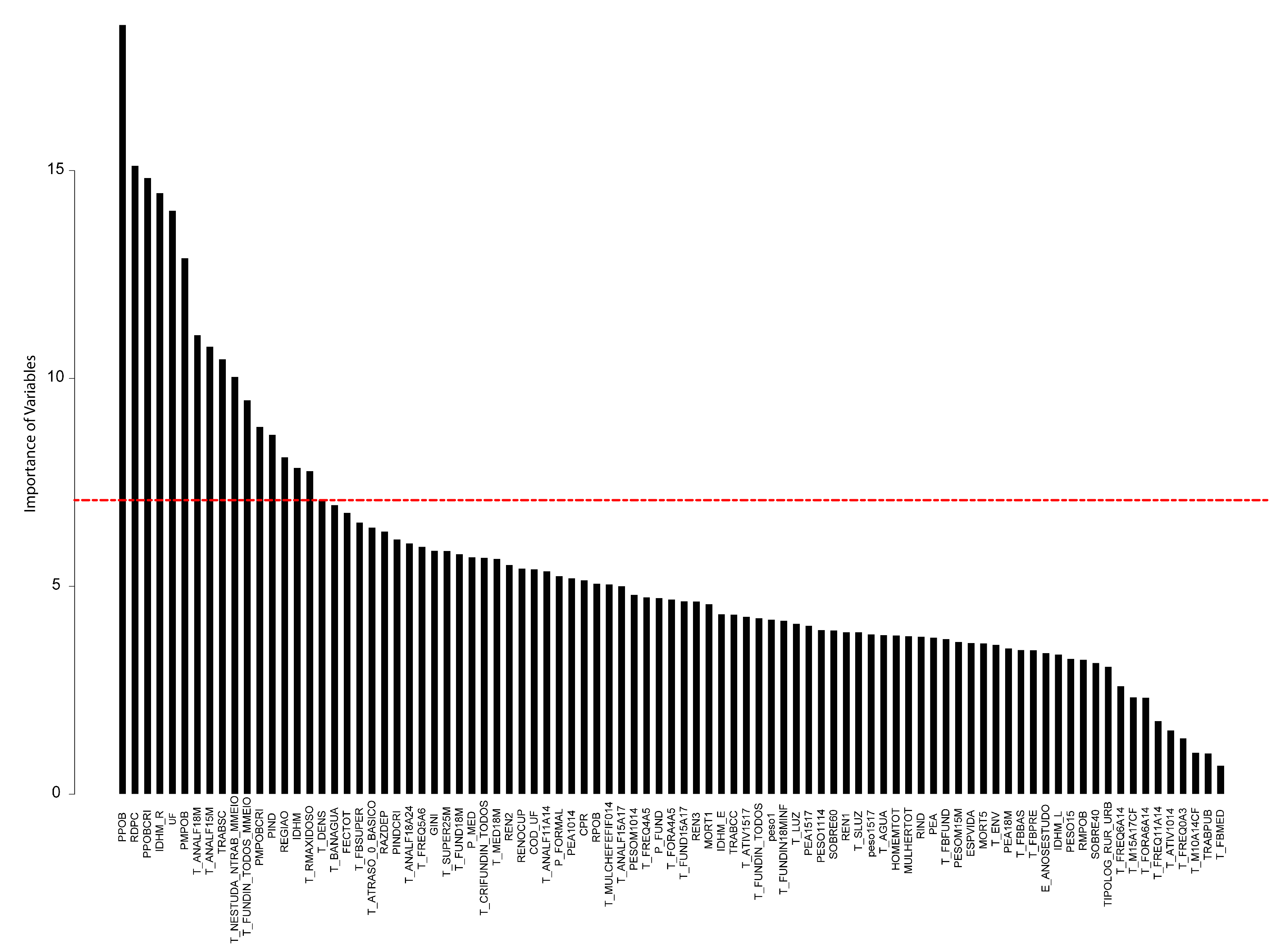
Subsequently, socioeconomic variables were considered in order to explain the utilization rate and a city database was prepared. Such variables are based on the variables collected in the 2010 Census and were taken from the portal of the [44] and from the [45], summing up a total of 89 covariates. A description of all of them can be found in the Appendix A. In this sense the modeling step was carried out, aiming to identify the variables that are possibly important for the use of the BFP. For this, two forms of modeling were performed: considering the response variable in its nature (regression) and in the categorized form (classification). The regression model correspond to response variable is continuous. The rate of use ($y_i$), defined as the number of people who use the assistance divided by the total population from that city, was estimated. Figure 6 shows the graph of the importance of the variables, with their respective cutoff in the variable selection.

The majority of the variables are continuous, with the exception $COD\_UF$ and $REGIAO$. Setting the y as target variable and the others variables as predictors, regression models were applied using Random Forest [34]. Its performance was evaluated using the Root Mean Squared Error (RMSE) which was calculated through a validation technique of 100 repeated holdout with split ratio of 70–30% training-test. This ratio was selected because provide a significant proportion sample [46].

The tuning of the hyperparameters used in the Random Forest algorithm estimation was realized through a grid search varying the following parameters: mtry—number of variables randomly sampled as candidates at each split ranges in $\{1;3;6\}$; nodesize—as the minimum size of observations in terminal nodes ranges in $\{5;10;25\}$; and ntree—as the number of tree collections in a Random Forest ranges in $\{100;500;1000\}$; The best combination of the hyperparameters was selected by the model which produced the lowest Root Mean Squared Error.

The result is summarized in the

Table 4. RMSE obtained by the Random Forest algorithm to estimate the rate of use ($y_i$) evaluated over the test data set.

	Mean	Median	SD
RMSE	0.0175	0.0175	0.0003

and express a great performance in order to solve the task of predict the rate of use ($y_i$) from different cities, which could represent a useful tool to guide the Government to better manage resources, and provide better support in directing public policies. The hyparameters that produced the lowest RMSE were $mtry=6$, $nodesize=25$ and $ntree=1000$.

The second modeling approach is a classification problem, resulting in the “Low” and “High” categories. The determination these categories from each state is given through the mean value of the BFP utilization rate, i.e., if a municipality has a BFP utilization rate lower than the mean value, it is labeled as “low” and, otherwise receive the “high” label. Moreover, the same tuning process was realized in order to select the better parameter’s setting the evaluation of the results were obtained using the same repeated holdout validation technique, with 100 repetitions and a split ratio of 70–30% of training-test data, but the metrics were the ACC, MCC and F1-Score.

Performance metrics of classification models are presented in

Table 5. Performance measures with selected variables.

Model	Accuracy		F1 Score		MCC
	Mean	SD	Mean	SD	Mean	SD
2 classes	0.9534	0.0039	0.9529	0.0039	0.9060	0.0078

. The hyper-parameters of RF which achieved there lowest generalization error were $mtry=4,nodesize=5,ntree=1000$. Beside its high predictive capacity, the Random Forest model also give an interpretation of the importance of each variable used to estimate the class of each city. Importance values use the Out-of-Bag (OOB) samples in its calculation. In each of those samples, a predictor was selected and its values were shuffled. Afterwards, the mean percentage of decreased accuracy’s value is obtained, and it is computed as the variable importance.

Table 6. Variables Importance in the classification model.

RANKING	VARIABLE	DESCRIPTION	V.IMP
1	PPOB	Proportion of people with per capita household income equal to or less than R$ 255.00 per month	30.77
2	UF	Federative Unity	24.72
3	RDPC	Average per capita income	20.99
4	PPOBCRI	Proportion of children vulnerable to poverty	20.61
5	IDHM_R	Municipal Human Development Index—Income Dimension	18.32
6	PMPOB	Proportion of people with per capita household income equal to or less than R$ 140.00 per month	16.30
7	TRABSC	% of employed persons aged 18 or over who are employed without a formal contract	13.73
8	T_DENS	Ratio between the total number of residents in the household and the total number of rooms used as a dormitory	13.73
9	T_ANALF15M	Illiteracy rate of the population aged 15 or over	13.53
10	T_ANALF18M	Illiteracy rate of the population aged 18 or over	13.08
11	REGIAO	Country Region	12.71
12	T_FUNDIN	% of people in households vulnerable to poverty and in whom no one has complete basic	10.78
13	T_RMAXIDOSO	% of people in households vulnerable to poverty and dependent on the elderly	10.76
14	IDHM	Municipal Human Development Index	9.93
15	T_NESTUDA	Proportion of young people aged 15 to 24 years old who do not study and do not work	9.01
16	PIND	Proportion of individuals with per capita household income equal to or less than R$ 70.00 per month	8.58
17	PMPOBCRI	Proportion of individuals up to 14 years of age who have per capita household income equal to or less than R $ 70.00 per month	8.47

represent an ranking of them based on the variable importance values. This information can add value in to formulation of public policy. From the result is clear that poverty is an important aspect in the attendance of the BFP program, therefore future design actions and plans can consider more targeted problems.

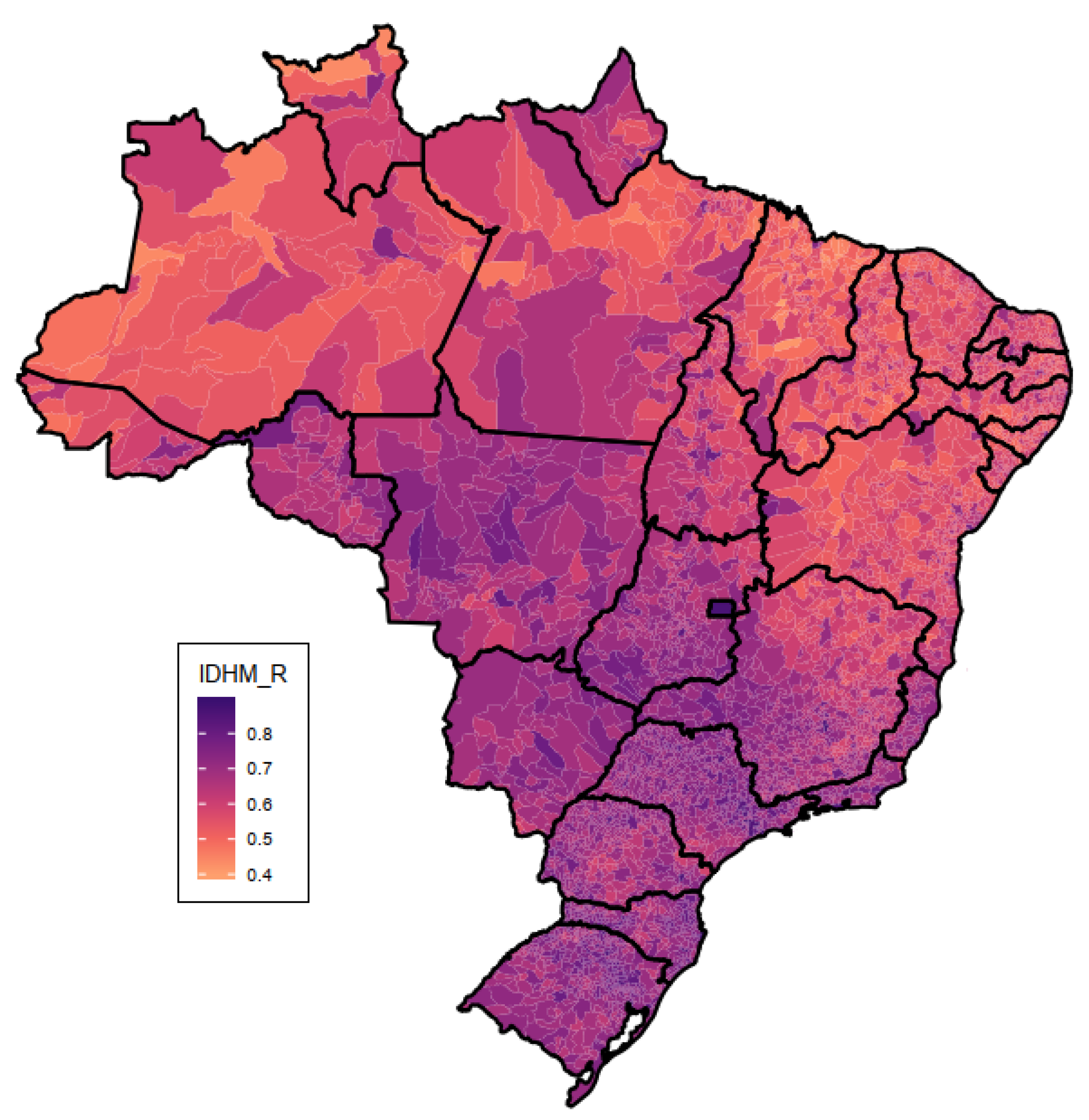
Moreover, the presence of the UF and REGIAO as high-rated importance variables can reveal an inequality between federative states and the Brazilian region, which is also an important feature to be analyzed through the government. Also, according to the Atlas of Human Development in Brazil (2019) [45], the IDHM_R is an indicator of the ability of the inhabitants of a locality to guarantee a proper standard that ensures their basic needs, for example, water, food and, housing. Thus, it can be seen from Figure 7 that the highest values refer to the states of the South, Southeast and Midwest regions of the country. Furthermore, this variable also plays a important role in the rate of use of BFP, due to appears at fifth on the variable importance ranking in Table 6.

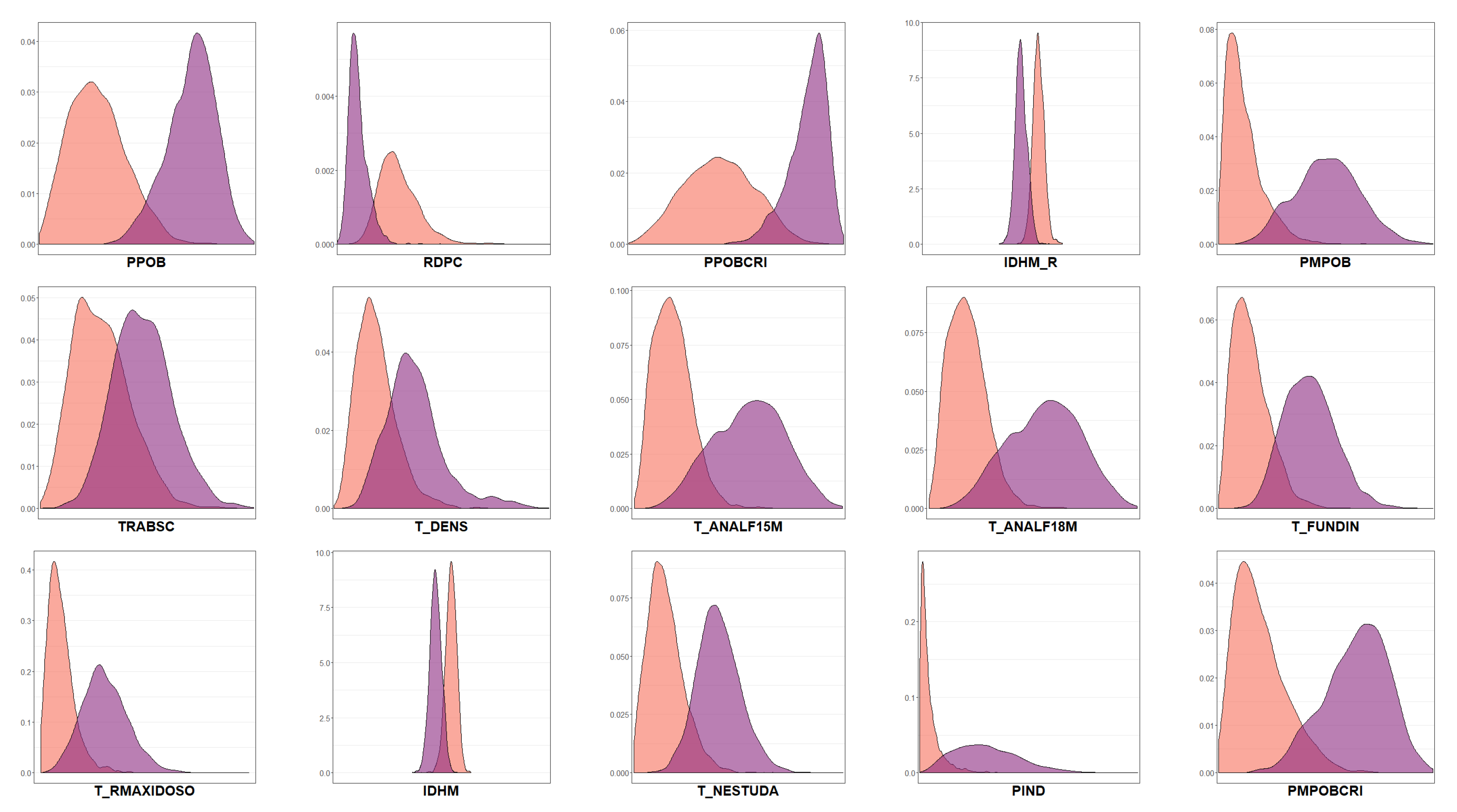
In order to verify the distribution behavior of the continuous variables over the binary utilization rate, Figure 8 displays a negative influence of RDPC, IDHM_R and IDHM and a positive influence of the other variables. This figure also corroborates the variable selection method used, since the distributions differ for the variable response.

5.3. Summary of Results

Through this analysis, it was possible to characterize the use of the program in Brazil and verify which are the cities, states, and regions with a low and high utilization rate of BF Program, as well as, through methods of selection of variables Random Forest, to identify important variables for the use of the BFP, such as the municipal human development index and the proportion of people vulnerable to poverty. Also, the analysis identifies as the most important the PPOB variable (Proportion of people with per capita household income equal to or less than R$255.00 per month) that gives us subsidies to believe in the effective action of the social program. Moreover, in addition to important factors such as income and education, this analysis draws attention to job informality and inactive youth, as measure by variables TRABSC (Percentage of people aged 18 or over who are employed without a formal contract) and T_NESTUDA (Proportion of young people aged 15 to 24 years old who do not study and do not work).

6. Final Considerations

For the Statistics community, R is one of the preferred tools. Despite its growth in the last years, it still has limitations for processing large volumes of data in single local machines. One way to perform statistical analyzes over massive databases is combining both tools (Spark and R) via the sparklyr package, which allows for a R application to use Spark.

In this paper, the implementation performed with the R software via the sparklyr package considered 111.6 GB of the monthly Brazilian public data from the Bolsa Família Program, which were processed on a local machine. Through the analysis it was possible to understand how this social program works in different cities, as well as to identify variables of great importance for the use of the program for example the variable that represents the proportion of young people aged 15 to 24 years who do not study and do not work.

Therefore, it is noted the potential of aggregating Spark and R for analysis of large databases, since in this work, using one local machine, was possible to analyze public data of large size, with about 1.26 billion observations, as well as providing important information which may subsidize national public management. Several future works may be considered in order to compare the time computational performance, other traditional statistical or machine learning models as well as time serial models to the monthly payments of the BFP.

References

1. Bhandarkar, M. MapReduce programming with apache Hadoop. In Proceedings of the 2010 IEEE International Symposium on Parallel & Distributed Processing (IPDPS), Atlanta, Georgia, USA, 19–23 April 2010; IEEE Computer Society: Piscataway, NJ, USA, 2010; p. 1. [Google Scholar]
2. Sagiroglu, S.; Sinanc, D. Big data: A review. In Proceedings of the 2013 International Conference on Collaboration Technologies and Systems (CTS), San Diego, CA, USA, 20–24 May 2013; IEEE: Piscataway, NJ, USA, 2013; pp. 42–47. [Google Scholar]
3. Caixa. 2019. Available online: http://www.caixa.gov.br/programas-sociais/bolsa-familia/Paginas/default.aspx (accessed on 20 April 2019).
4. Citizenship, M. Special Secretariat for Social Development. Ministry of Citizenship. 2019. Available online: http://mds.gov.br/assuntos/bolsa-familia/o-que-e/como-funciona/como-funciona (accessed on 29 April 2019).
5. Hummon, N.P.; Fararo, T.J. Actors and networks as objects. Soc. Netw. 1995, 17, 1–26. [Google Scholar] [CrossRef]
6. Expósito, O.Á. Guide to Spark Machine Learning for Credit Scoring. Bachelor’s Thesis, Universitat Politècnica de Catalunya, Barcelona, Spain, 2018. [Google Scholar]
7. Hadoop. Apache Software Foundation. Apache Hadoop. 2019. Available online: http://hadoop.apache.org/ (accessed on 20 May 2019).
8. Spark. Apache Software Foundation. Apache Spark. 2019. Available online: http://spark.apache.org/ (accessed on 20 May 2019).
9. Zaharia, M.; Chambers, B. Spark: The Definitive Guide; O’Reilly: Sevastopol, CA, USA, 2018; Available online: https://learning.oreilly.com/library/view/spark-the-definitive/9781491912201/ (accessed on 29 June 2019).
10. Luraschi, J.E.A.; Kuo, K.; Ushey, K.; Allaire, J.; Macedo, S.; Falaki, H.; Wang, L.; Zhang, A.; Li, Y. The Apache Software Foundation Package ‘Sparklyr’. Available online: https://cran.r-project.org/web/packages/sparklyr/index.html (accessed on 15 April 2019).
11. Bluhm, B.; Cutura, J. Econometrics at Scale: Spark Up Big Data in Economics; Technical Report; SAFE Working Paper No. 266; Leibniz Institute for Financial Research SAFE: Frankfurt, Germany, 2020. [Google Scholar]
12. Safhi, H.M.; Frikh, B.; Ouhbi, B. Energy load forecasting in big data context. In Proceedings of the 2020 5th International Conference on Renewable Energies for Developing Countries (REDEC), Marrakech, Morocco, 24–26 March 2020; IEEE: Piscataway, NJ, USA, 2020; pp. 1–6. [Google Scholar]
13. Hales, D.; Patarin, S. Computational sociology for systems “in the wild”: The case of BitTorrent. IEEE Distrib. Syst. Online 2005, 6. [Google Scholar] [CrossRef]
14. Victorino, M.; de Holanda, M.T.; Ishikawa, E.; Oliveira, E.C.; Chhetri, S. Transforming Open Data to Linked Open Data Using Ontologies for Information Organization in Big Data Environments of the Brazilian Government: The Brazilian Database Government Open Linked Data–DBgoldbr. Knowl. Organ. 2018, 45, 443–466. [Google Scholar] [CrossRef]
15. Schwartzman, S. Education-Oriented Social Programs in Brazil: The Impact of Bolsa Escola. In Paper Submitted to the Global Conference on Education Research in Developing Countries (Research for Results on Education), Global Development Network, Prague, 32 March–2 April 2005; Instituto de Estudos do Trabalho e Sociedade: Rio de Janeiro, Brazil, 2005. [Google Scholar]
16. Ferro, A.R.; Kassouf, A.L.; Levison, D. The impact of conditional cash transfer programs on household work decisions in Brazil. In Child Labor and the Transition between School and Work; Emerald Group Publishing Limited: Bingley, UK, 2010. [Google Scholar]
17. Magalhães, L.A.; Fonseca, M.F.; Custodio, D.D.O.; Martinho, P.; Daltio, J.; de Carvalho, C.; Castro, G. Gathering spatial data on social vulnerability in Brazil. Embrapa Territorial-Artigo em anais de congresso (ALICE). In Proceedings of the International Conference on Agro Big Data and Decision Support Systems, Montevideo, Uruguay, 27–29 September 2017; pp. 183–185. [Google Scholar]
18. Shoro, A.G.; Soomro, T.R. Big data analysis: Apache spark perspective. Glob. J. Comput. Sci. Technol. 2015, 15, No 1-C. [Google Scholar]
19. Mavridis, I.; Karatza, H. Performance evaluation of cloud-based log file analysis with Apache Hadoop and Apache Spark. J. Syst. Softw. 2017, 125, 133–151. [Google Scholar] [CrossRef]
20. Alsheikh, M.A.; Niyato, D.; Lin, S.; Tan, H.P.; Han, Z. Mobile big data analytics using deep learning and apache spark. IEEE Netw. 2016, 30, 22–29. [Google Scholar] [CrossRef] [Green Version]
21. Alexopoulos, A.; Drakopoulos, G.; Kanavos, A.; Mylonas, P.; Vonitsanos, G. Two-Step Classification with SVD Preprocessing of Distributed Massive Datasets in Apache Spark. Algorithms 2020, 13, 71. [Google Scholar] [CrossRef] [Green Version]
22. Gopalani, S.; Arora, R. Comparing apache spark and map reduce with performance analysis using k-means. Int. J. Comput. Appl. 2015, 113, 8–11. [Google Scholar] [CrossRef]
23. Yu, J.; Zhang, Z.; Sarwat, M. Spatial data management in apache spark: The geospark perspective and beyond. Geoinformatica 2019, 23, 37–78. [Google Scholar] [CrossRef]
24. Azevedo, A.R.; Ara, A.; Noguti, M.Y.; de Brito, A.C. Application in Shiny: Intersection between gender, class, and race at ENEM 2016. In Proceedings of the III International Statistics Seminar with R, Niterói, RJ, Brazil, 22–24 May 2018. [Google Scholar]
25. Brent, E.E., Jr. Computational sociology: Reinventing sociology for the next millennium. Soc. Sci. Comput. Rev. 1993, 11, 487–499. [Google Scholar] [CrossRef]
26. Hummon, N.P.; Fararo, T.J. The emergence of computational sociology. J. Math. Sociol. 1995, 20, 79–87. [Google Scholar] [CrossRef]
27. Salgado, M.; Gilbert, N. Emergence and communication in computational sociology. J. Theory Soc. Behav. 2013, 43, 87–110. [Google Scholar] [CrossRef] [Green Version]
28. White, T. Hadoop: The Definitive Guide; O’Reilly Media, Inc.: Sevastopol, CA, USA, 2015. [Google Scholar]
29. Grover, M.; Malaska, T.; Seidman, J.; Shapira, G. Hadoop Application Architectures: Designing Real-World Big Data Applications; O’Reilly Media, Inc.: Sevastopol, CA, USA, 2015. [Google Scholar]
30. Pattamsetti, R.M.R. Distributed Computing in Java 9; Packt Publishing Ltd.: Birmingham, UK, 2017. [Google Scholar]
31. Zaharia, M.; Xin, R.S.; Wendell, P.; Das, T.; Armbrust, M.; Dave, A.; Meng, X.; Rosen, J.; Venkataraman, S.; Franklin, M.J.; et al. Apache spark: A unified engine for big data processing. Commun. ACM 2016, 59, 56–65. [Google Scholar] [CrossRef]
32. R, C. R: A Language and Environment for Statistical Computing; R Foundation for Statistical Computing: Vienna, Austria, 2019. [Google Scholar]
33. Luraschi, J.; Kuo, K.; Ruiz, E. Mastering Spark with R: The Complete Guide to Large-Scale Analysis and Modeling; O’Reilly Media: Sevastopol, CA, USA, 2019. [Google Scholar]
34. Breiman, L. Random forests. Mach. Learn. 2001, 45, 5–32. [Google Scholar] [CrossRef] [Green Version]
35. Zadrozny, B. Learning and evaluating classifiers under sample selection bias. In Proceedings of the twenty-first international conference on Machine learning, Banff, AB, Canada, 4–8 July 2004; p. 114. [Google Scholar]
36. Breiman, L. Bias, Variance, and Arcing Classifiers; Technical Report; Tech. Rep. 460; Statistics Department, University of California, Berkeley: Berkeley, CA, USA, 1996. [Google Scholar]
37. Dmitrievsky, M. Random Decision Forest in Reinforcement Learning; MetaQuotes Language 5 (MQL5); 2018. Available online: https://www.mql5.com/en/articles/widget/3856 (accessed on 23 September 2019).
38. Genuer, R.; Poggi, J.M.; Tuleau-Malot, C. Variable selection using random forests. Pattern Recognit. Lett. 2010, 31, 2225–2236. [Google Scholar] [CrossRef] [Green Version]
39. Refaeilzadeh, P.; Tang, L.; Liu, H. Cross-Validation. Encycl. Database Syst. (EDBS) 2009, 5, 532–538. [Google Scholar]
40. Tantithamthavorn, C.; McIntosh, S.; Hassan, A.E.; Matsumoto, K. An empirical comparison of model validation techniques for defect prediction models. IEEE Trans. Softw. Eng. 2016, 43, 1–18. [Google Scholar] [CrossRef]
41. Chicco, D.; Jurman, G. The advantages of the Matthews correlation coefficient (MCC) over F1 score and accuracy in binary classification evaluation. BMC Genom. 2020, 21, 6. [Google Scholar] [CrossRef] [PubMed] [Green Version]
42. Allaire, J.J. Rstudio. 2009. Available online: https://www.rstudio.com/about/ (accessed on 10 May 2019).
43. Portal. Transparency Portal; General Controller of the Union 2019. Available online: http://www.portaltransparencia.gov.br/download-de-dados/bolsa-familia-pagamentos/ (accessed on 28 April 2019).
44. IBGE. Brazilian Institute of Geography and Statistics; IBGE 2019. Available online: http://www.ibge.gov.br (accessed on 15 May 2019).
45. Atlas. The IDHM. Atlas of Human Development in Brazil 2019. Available online: http://www.atlasbrasil.org.br/2013/pt/o_atlas/metodologia/idhm_renda/ (accessed on 5 June 2019).
46. Larsen, J.; Goutte, C. On optimal data split for generalization estimation and model selection. In Proceedings of the Neural Networks for Signal Processing IX: Proceedings of the 1999 IEEE Signal Processing Society Workshop (Cat. No.98TH8468), Madison, WI, USA, 25 August 1999; pp. 225–234. [Google Scholar]
Figure 1. General structure of a random forest model. Source: adapted from [37] and prepared by the authors.
Stats 03 00028 g001
Figure 2. General utilization rate of BFP over the months. Source: prepared by the authors.
Stats 03 00028 g002
Figure 3. Distribution of the average of BFP city utilization rate. Source: prepared by the authors.
Stats 03 00028 g003
Figure 4. Map of the average city use rates of the BFP in 2019, for 2 classes. Source: prepared by the authors.
Stats 03 00028 g004
Figure 5. Utilization rate of BFP with two classes by state. Source: prepared by the authors.
Stats 03 00028 g005
Figure 6. Importance of variables with cutoff point via CART regression modeling. Source: prepared by the authors.
Stats 03 00028 g006
Figure 7. An overview of IDHM_R in Brazil. Source: prepared by the authors.
Stats 03 00028 g007
Figure 8. The distribution behavior of some variables over the binary utilization rate in Brazil. Source: prepared by the authors.
Stats 03 00028 g008