Identification of Judicial Outcomes in Judgments: A Generalized Gini-PLS Approach

Abstract

This paper presents and compares several text classification models that can be used to extract the outcome of a judgment from justice decisions, i.e., legal documents summarizing the different rulings made by a judge. Such models can be used to gather important statistics about cases, e.g., success rate based on specific characteristics of cases’ parties or jurisdiction, and are therefore important for the development of Judicial prediction not to mention the study of Law enforcement in general. We propose in particular the generalized Gini-PLS which better considers the information in the distribution tails while attenuating, as in the simple Gini-PLS, the influence exerted by outliers. Modeling the studied task as a supervised binary classification, we also introduce the LOGIT-Gini-PLS suited to the explanation of a binary target variable. In addition, various technical aspects regarding the evaluated text classification approaches which consists of combinations of representations of judgments and classification algorithms are studied using an annotated corpora of French justice decisions.

1. Introduction

Judicial prediction is the ability to predict what a judge will decide on a given case. Is it possible to develop efficient predictive models to automatize such predictions? This question has long been driving several initiatives at the crossroads of Artificial Intelligence and Law—in particular, through the development of predictive models based on the alignment of computable features of the case that were available to the judge prior to the judgment, with computable features of the judge’s decision on the case. In this line of work, this paper presents a study towards the development of such predictive models taking advantage of Machine Learning and Natural Language Processing techniques. The legal vocabulary being notoriously ambiguous, we first detail important concepts that will be used thereafter.

A case begins with a complaint requesting a remedy for harm suffered due to the wrongdoing of the defendant. The features of the case are the circumstances existing prior to the filing of the complaint that is a set of facts sufficient to justify a right to file a complaint.

A claim is a request made by a plaintiff against a defendant, seeking legal remedy. Claims can be grouped into different categories, depending on the rule applicable and the type of remedy sought (e.g., injunctive relief, cease and desist order, damages).

A judgment summarizes the different rulings made by a judge about a certain case into a document. Judgments therefore contain many features that can be extracted (e.g., type of court, name of the parties, claims made by the parties, judges decisions on the claims). A complaint is a judgment that can contain many different claims, seeking different types of remedy. Therefore, in general, a judgment concern different types of claims.

The decision is a ruling made on a particular claim. We further consider that the judges decision on a claim is either accepted or rejected. Note that a judgment must be distinguished from the judge’s decision on a specific claim.

In recent years, the methodology of judicial predictions were mostly exclusively based on the employ of neural networks, which may be seen as the most flexible models for classification and predictions of legal decisions when large datasets are available. Chalkidis and Androutsopoulos [1] use a Bi-LSTM network running on words on a task of extracting contractual clauses. Wei et al. [2] have shown the superiority of convolutional networks over Support Vector Machines for the classification of texts on large specific datasets. The use of a Bi-GRU has become a standard approach, see [3]. Performance of 92% was obtained on the identification of criminal charges and on judicial outcomes from Chinese criminal decisions [4]. These types of approaches can also be used successfully on judgments in civil matters [5]. Bi-LSTM networks coupled with a representation of the judgment in the form of a tensor achieve performance around 93% on a corpus of 1.8 million Chinese criminal judgments [6]. This work has been successfully replicated on a body of judgments of the European Court of Human Rights in English, with F-measure performance of 80% for bi-GRU networks with attention and Hierarchical BERT [7]. On the same corpus, the development of a specific lexical embedding ECHR2Vec makes it possible to reach performances around 86% [8]. Similar performances of 79% are obtained by TF-IDF (Term Frequency-Inverse Document Frequency) in the Portuguese language [9]. Although neural networks enable very good performances to be achieved, we defend in this paper the use of compression machine learning models based on word representations such as TF-IDF with different variants corresponding to different weighting schemes. These approaches are particularly suited dealing with small- to medium-size annotated datasets.

As we stressed, claims can be grouped into specific categories depending on their nature, e.g., several claims may refer to the notion of child care; such categories are defined a priori by jurists for the analysis of a corpus of judgments of interest. In addition, a judgment most of the time only contains a single claim of a given category (A corpus description and a descriptive analysis are provided in the next section). In this context, we are interested in the definition of predictive models able to predict the judge’s decision expressed in a judgment for a specific category of claims. Stated otherwise, knowing that a judgment contains a single claim of a given category, the model will have to answer the following question analyzing the judgment (textual document): has the claim been accepted or rejected? Developing efficient predictors of the outcome of specific categories of claims is of major interest for the analysis of large corpus of judgments. It, for instance, paves the way for large statistical analysis of correlations between aspects of the case (e.g., parties, location of the court) and outcomes for specific categories of claims. Such analyses are important for theoretical studies on law enforcement and future development of models able to predict the outcome of cases. Note that traditional text classification techniques obtain good performance predicting if a judgment contains a claim of a specific category, see [10]. Obtaining relevant statistics about judge’s decisions on a given category of claim would therefore be based on (i) applying the aforementioned model to distinguish judgments containing a claim of the category of interest, and (ii) applying the type of models studied in this paper to know the outcome of previously identified judgments.

The methodology of judicial predictions therefore depends on the ability of a model to predict the judge’s decision on a claim inherent to a given category—without knowing the precise localization of the statement of the judge’s decision inside a judgment. In this context, extracting the result of a claim can be formulated as a task of binary text classification. To tackle this task, we consider in this paper the supervised machine learning paradigm assuming that a set of annotated judgments, i.e., labelled dataset, is provided for each category of claims of interest. We therefore aim to use the labeled dataset for training an algorithm to recognize whether the request has been rejected or accepted. Considering this setting, the paper presents various models and empirically compares them on a corpus of French judgments. A statistical analysis of the impact of various technical aspects generally involved in the classification of texts which consists of a combination of representations of judgments and classification algorithms is proposed. This analysis sheds light on certain configurations making it possible to determine judges’ decisions of a claim. We also propose the generalized Gini-PLS algorithm which is an extension of the simple Gini-PLS model [11]. This generalized Gini-PLS consists in adding a regularization parameter that makes it possible to better adapt the regression with respect to the information in the distribution tails while attenuating, as in the simple Gini-PLS, the influence exerted by outliers. We also propose a new regression (LOGIT-Gini-PLS) which is better suited to the explanation of a target variable when the latter is a binary variable. These two models have never been applied to text classification.

The paper is organized as follows: Section 2 presents characteristics of the corpus used for this study and motivates the modeling of the task adopted in this paper (i.e., decision outcome prediction as a binary text classification). Section 3 presents the different TF-IDF vectorizations of the judgments. Section 4 presents the proposed generalized (LOGIT) Gini-PLS algorithms for text classification. Section 5 presents our experiments and results. Section 6 concludes our study.

2. Datasets and Modeling Motivations

We assume in this paper that predicting judges decisions may be studied through the lens of the definition of binary text classification models. This positioning is based on discussions with jurists and motivated by analyses performed on labeled datasets of French judgments. Six datasets built from a corpus of French judgments are considered in our study, one for each of the six categories of claims introduced in

Table 1. Categories of claims of the study.

Dataset	Description	Number of Judgments
ACPA	Civil fine for abuse of process	246
CONCDEL	Damages for unfair competition	238
DANAIS	Damages for abuse of process	421
DCPPC	declaration of claim to liabilities of the collective procedure	218
DORIS	damages for neighborhood disturbance	164
STYX	irrecoverable expenditure	123

.

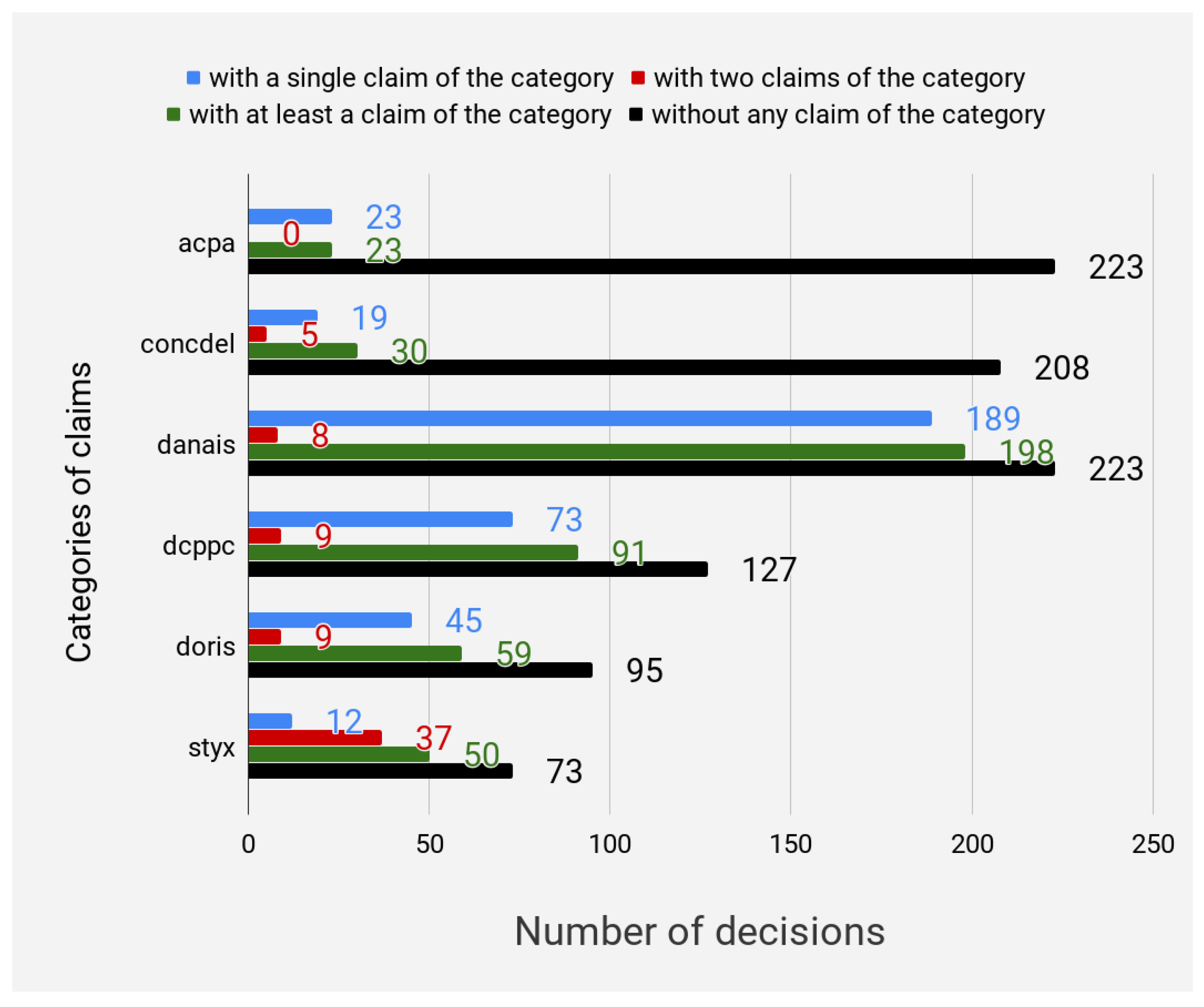
The semantics of the membership of a judgments into a category is: the judgments contain a claim of that category, i.e., all the judgments into the ACPA category contain a claim related to Civil fine for abuse of process.

Table 2. Extract from “Cour d’appel, Paris, Pôle 6, chambre 9, 18 Mai 2016 n° 14/11380”.

	In French	In English
claim	l’audience, la SA SFP reprenant oralement ses conclusions vises par le greffier, result la cour de: - confirmer le jugement dfr-dbouter M. S. de l’ensemble de ses demandes - le condamner payer une amende civile de 1.500 € pour procdure abusive en application de l’article 32-1 du code de procdure civile - le condamner payer la somme...	At the hearing, SA SFP orally resuming its conclusions referred to in the clerk, requests the court to: - confirm the judgment referred - dismiss Mr S. of all his requests - order him to pay a civil fine of €1500 for abusive procedure in application of article 32-1 of the code of civil procedure - order him to pay the sum…
decision	PAR CES discussion LA COUR, CONFIRME le jugement dfr en toutes ses dispositions; Y ajoutant, DIT n’y avoir lieu application des dispositions de l’article 700 du code de procdure civile; REJETTE le surplus des demandes; CONDAMNE M Khellil S. aux dpens d’appel.	FOR THESE REASONS THE COURTYARD, CONFIRMS the judgment referred in all its provisions; Adding to it, SAID to take place there in application of the provisions of article 700 of the code of Civil Procedure; REJECTS excess requests; ORDERS M Khellil S. at costs of appeal.

presents sections of a judgment of that category [ACPA]. The sections refer to the mentions of the claim and to the corresponding decision, respectively. Figure 1 presents additional details about the datasets, in particular the number of claims of a category found in the judgments.

Observation 1.

Decisions most often only contain a single claim of a specific category.

On the one hand, the statistics on the labelled data show that the judgments contain for the most part a single claim of a category (or at least one claim of the category). The percentage of judgments having only one request of a category is respectively: 100% for ACPA, 63.33% for CONCDEL, 95.45% for DANAIS, 80.22% for DCPPC, and 76.21% for DORIS. However, we note the exception of the STYX category (damages on article 700 CPC), where, in most of the judgments, there are instead two claims. This exception can be justified by the fact that each party generally makes this type of request because it relates to the reimbursement of legal costs.

On the other hand, few judgments with two or more claims exist. In this case, the classification task of any claim becomes difficult since specific vocabulary and sentences may appear in the judgment related to other claims (although there are in the same category). This may be embodied by noise or outliers in the dataset of each claim category. The use of Gini estimators is therefore welcome to handle outlying observations.

Observation 2.

Most judges’ decisions are binary: accept or reject.

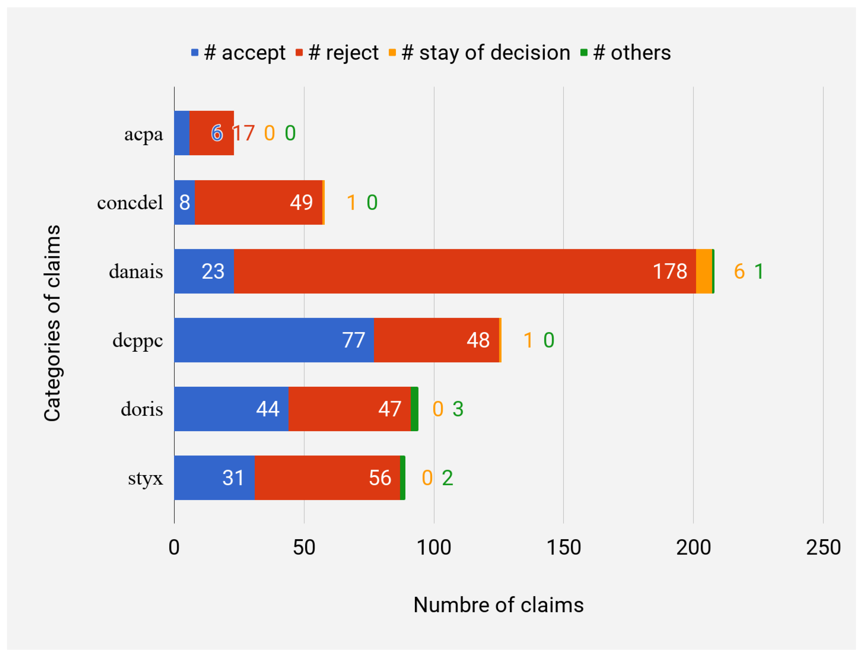
Figure 2 highlights the fact that outcomes of a given claim are most often accepted or rejected, and that other forms of results are very rare. Theses observations motivate the interest of developing a binary classifier for predicting the outcome of a claim appertaining to a specific category.

Observation 3.

The algorithm must be able to deal with a large number of tokens of judgments.

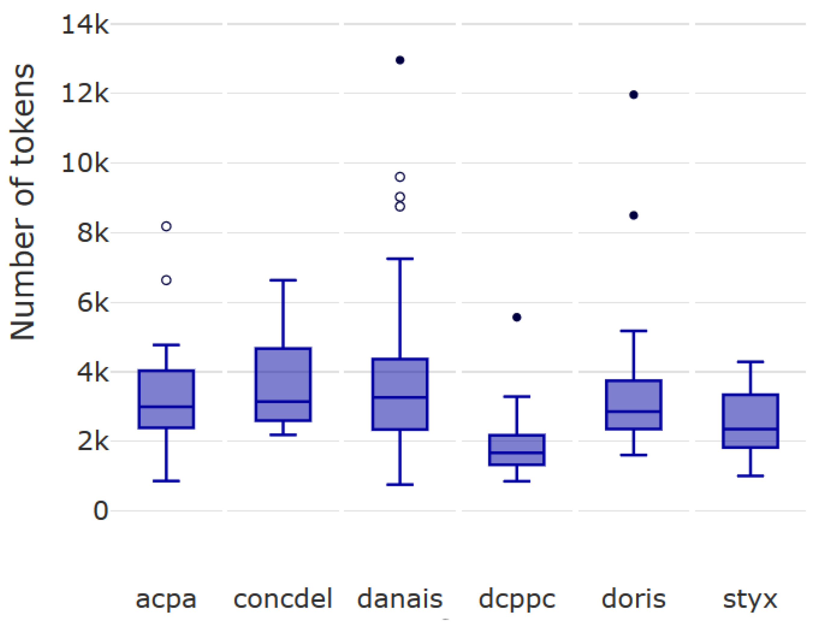
Figure 3 illustrates the distribution of the judgments’ lengths (number of tokens, i.e., words). We note that the texts are long in comparison to those usually considered by state-of-the-art text classification approaches. As we will discuss later, this particularity will hamper the use of some efficient existing approaches such as PLS algorithms for compression.

Observation 4.

In some claim categories, a strong imbalance may exist between the outcomes accept/reject.

Table 3. Class distributions per claim category.

Dataset	Accepted	Rejected	Total
ACPA	6 (26.09%)	17 (73.91%)	23
CONCDEL	4 (22.22%)	14 (77.78%)	18
DANAIS	21 (11.23%)	166 (88.77%)	187
DCPPC	48 (66.66%)	24 (33.33%)	72
DORIS	23 (52.27%)	21 (47.72%)	44
STYX	4 (33.33%)	8 (66.67%)	12

presents the final statistics of the dataset used for both training and evaluating the predictive models evaluated in this study. As can be seen, four claim categories out of six exhibit strong unbalanced decisions.

3. Texts Classification

Text classification allows judgments to be organized in predefined groups. This technique has received a large audience for a long time. Two technical choices mainly influence the performance of the classification: the representation of the texts and the choice of the classification algorithm. In the following, the predicted variable is denoted y, the predictors are denoted x, the learning base including the observations of the sample is expressed as $D=\{{(x_i,y_i)}_{i=1...N}\}$, and C represents claim categories.

Considering a vocabulary $V=\{t_1,t_2,\cdots ,t_n\}$, we further assume that every judgment $d\in D$ is represented as a TF-IDF vector embedding (Term Frequency-Inverse Document Frequency) [12]$\overrightarrow{d}\in {\mathbb{R}}^n$, where each dimension $1\le k\le n$ refers to word $t_k\in V$ and $\overrightarrow{d}\left[k\right]=w(t_k,d)$ is the weight of $t_k$ in d defined as the normalized product of a global weight $g\left(t_k\right)$ depending on the training corpus and a local weight $l(t_k,d)$ stressing the importance of $t_k$ in judgment d:

$$w(t_k,d)=l(t_k,d)\times g\left(t_k\right)\times nf\left(d\right)$$

with $nf$ a normalization factor.

Table 4. Notation used in formulas.

Notation	Description
t	a term
d	a judgment (document)
$\left|d\right|$	size of d (number of tokens)
c	a label
$\overline{c}$	the other labels
D	the global set of documents ($N=\left|D\right|$)
$D_c$	the set of documents labeled with c
$D_{\overline{c}}$	the set of documents not labeled with c
$N_t$	the number of documents containing t
$N_{\overline{t}}$	the number of documents without t
$N_{t,c}$	the number of documents of c with t
$N_{\overline{t},c}$	the number of documents of c without t
$N_{t,\overline{c}}$	the number of documents of $\overline{c}$ with t
$N_{\overline{t},\overline{c}}$	the number of documents of $\overline{c}$ without t
$D{F}_{t|c}$	proportion of documents of c with t ($D{F}_{t|c}=\frac{N_{t,c}}{|D_c|}$)
$D{F}_{c|t}$	proportion of documents of c in the global set of documents with t

summarizes the notations used in the paper. The global weight is computed following one of the methods presented in

Table 5. Global weighting metrics.

Description	Formula
Inverse document frequency (IDF) [13]	$idf\left(t\right)={log}_2\left(\frac{N}{N_t}\right)$
Probabilistic IDF [14]	$pidf\left(t\right)={log}_2\left(\frac{N}{N_t}-1\right)$
BM25 IDF [15]	$bidf\left(t\right)={log}_2\left(\frac{N_{\overline{t}}+0.5}{N_t+0.5}\right)$
Frequency difference	${\Delta }_{DF}(t,c)=D{F}_{t|c}-D{F}_{t|\overline{c}}$
Information gain [16]	$ig(t,c)=$ $$\frac{N_{t,c}}{N}{log}_2\left(\frac{N_{t,c}N}{N_t}\right)+\frac{N_{\overline{t},c}}{N}{log}_2\left(\frac{N_{\overline{t},c}N}{N_{\overline{t}}\left|D_c\right|}\right)+\frac{N_{t,\overline{c}}}{N}{log}_2\left(\frac{N_{t,\overline{c}}N}{N_t\left|D_{\overline{c}}\right|}\right)+\frac{N_{\overline{t},\overline{c}}}{N}{log}_2\left(\frac{N_{\overline{t},\overline{c}}N}{N_{\overline{t}}\left|D_c\right|}\right)$$
Relevance frequency [17]	$rf(t,c)=log\left(2+\frac{N_{t,c}}{max(1,N_{t,\overline{c}})}\right)$
${\chi }^2$ coefficient [18]	${\chi }^2(t,c)=\frac{N{(\left(N_{t,c}{N}_{\overline{t},\overline{c}}\right)-\left(N_{t,\overline{c}}{N}_{\overline{t},c}\right))}^2}{N_t{N}_{\overline{t}}|D_c\left|\right|D_{\overline{c}}|}$
Correlation coefficient [19]	$ngl(t,c)=\frac{\sqrt{N}\left(N_{t,c}{N}_{\overline{t},\overline{c}}\right)-\left(N_{t,\overline{c}}{N}_{\overline{t},c}\right)}{\sqrt{N_t{N}_{\overline{t}}|D_c\left|\right|D_{\overline{c}}|}}$
GSS coefficient [20]	$gss(t,c)=\left(N_{t,c}{N}_{\overline{t},\overline{c}}\right)-\left(N_{t,\overline{c}}{N}_{\overline{t},c}\right)$
Marascuilo coefficient [21]	$mar(t,c)=\frac{\left(\begin{array}{l}{(N_{t,c}-N_t{N}_{t,c}/N)}^2\\ +(N_{t,\overline{c}}-N_t|D_{\overline{c}}{|/N)}^2\\ +(N_{\overline{t},c}-|D_c{|N_{\overline{t}}/N)}^2\\ +(N_{\overline{t},\overline{}}-N_{\overline{t}}|D_{\overline{c}}{|/N)}^2\end{array}\right)}{N}.$
Smoothed IDF delta [22]	$dsidf(t,c)={log}_2\left(\frac{|D_{\overline{c}}|(N_{t,c}+0.5)}{|D_c|(N_{t,\overline{c}}+0.5)}\right)$
BM25 IDF delta [22]	$dbidf(t,c)={log}_2\left(\frac{\left(\right|D_{\overline{c}}|-N_{t,\overline{c}}+0.5\left)\right|(N_{t,c}+0.5)}{\left(\right|D_c|-N_{t,c}+0.5)(N_{t,\overline{c}}+0.5)}\right)$

. The local weight is computed from the frequency of occurrences of the word in the judgment using one of the methods of

Table 6. Local weighting metrics.

Description	Formula
Gross term statement [12]	$tf(t,d)=$ Number of occurrences of t in d
Presence of the word [12]	$tp(t,d)=\left\{\begin{array}{cc}1& \mathrm{if}tf(t,d)>0\hfill \\ 0& \mathrm{otherwise}\hfill \end{array}\right.$
Log Normalization	$logtf(t,d)=1+log\left(tf(t,d)\right)$
Increased and standardized frequency of the word [12]	$atf(t,d)=k+(1-k)\frac{tf(t,d)}{\underset{t\in V}{max}tf(t,d)}$
Normalization based on the average frequency of the word [23] ($avg$ is the average)	$logave(t,d)=\frac{1+logtf(t,d)}{1+logav{g}_{t\in V}tf(t,d)}$

.

The vector representation of texts generally results in high-dimensional vectors whose coordinates are mostly zero. Consequently, dimension reduction (compression) techniques, such as PLS regressions, make it possible to obtain vectors more relevant to classification tasks.

4. Generalized Gini-PLS Algorithms for Text Classification

The Gini-PLS regression was introduced by [11]. In what follows, we propose two Gini-PLS algorithms: a generalized Gini-PLS regression based on the Gini generalized covariance operator, and a combination of the latter to the logistic regression. We first review the PLS algorithm.

4.1. PLS

The advantage of the Gini-PLS algorithm is to reduce the sensitivity to outliers. It is an extension of the PLS analysis (partial least square) [24]. The PLS analysis explains the dependence between one or more predicted variables y and predictors $\mathbf{x}=(x_1,x_2,\cdots ,x_m)$. It mainly consists in transforming the predictors into a reduced number of h orthogonal principal components $t_1,\cdots ,t_h$. It is therefore a method of dimension reduction in the same way as principal components analysis (PCA), linear discriminant analysis (LDA), and quadratic discriminant analysis (QDA). The components $t_1,\dots ,t_h$ are built in different steps by applying the PLS algorithm repeatedly. More precisely, at each iteration $i\in [1,h]$, the component $t_i$ is calculated by the formula $t_i=\mathbf{x}·{\mathbf{w}}_i$, and then the target y is regressed by OLS on $\mathbf{x}$. PLS analysis has several advantages [25] including robustness to the high-dimensional problem and the ability to eliminate the multicollinearity problem [26]. These problems are likely to arise on small corpora of texts with a large number of words as in our case. The PLS method is extended and successfully applied for various regression problems [25] or classification of data in general [27,28,29], and of texts in particular [30].

4.2. The Gini Covariance Operator

Schechtman and Yitzhaki [31] have recently generalized the Gini covariance operator, i.e., co-Gini, in order to impose more or less weight at the tails of distributions. This Gini covariance operator is given by:

$$\mathrm{cog}(x_{\ell },x_k):=\mathrm{cov}(x_{\ell },F\left(x_k\right))=\frac{1}{N}\sum _{d=1}^N(x_{d\ell }-\overline{x_{\ell }})(F\left(x_{dk}\right)-{\overline{F}}_{x_k}),$$

(1)

where $F\left(x_k\right)$ is the cdf of variable $x_k$. Let us denote $r_k=(R_{\downarrow }\left(x_{1k}\right),\dots ,R_{\downarrow }\left(x_{Nk}\right))$ the vector decreasing rank of variable $x_k$, in other words, the vector which assigns the lowest rank (1) of the observation with the highest value $x_{dk}$, and so on:

$$R_{\downarrow }\left(x_{dk}\right):=\left\{\begin{array}{cc}N+1-\#\{x\le x_{dk}\}\hfill & \mathrm{no}\mathrm{similar}\mathrm{observation}\hfill \\ N+1-\frac{{\sum }_{d=1}^p\#\{x\le x_{dk}\}}{p}\hfill & \mathrm{if}p\mathrm{similar}\mathrm{observations}{x}_{dk}.\hfill \end{array}\right.$$

The generalized co-Gini operator is given by Schechtman and Yitzhaki [31]:

$${\mathrm{cog}}_{\nu }(x_{\ell },x_k):=-\nu \mathrm{cov}(x_{\ell },r_k^{\nu -1});\nu >1.$$

(2)

The role of the co-Gini operator can be explained as follows. When $\nu \to 1$, the variability of the variables is attenuated so that ${\mathrm{cog}}_{\nu }(x_k,x_{\ell })$ tends to zero (even if the variables $x_k$ and $x_{\ell }$ are strongly correlated). On the contrary, if $\nu \to \infty$, then ${\mathrm{cog}}_{\nu }(x_k,x_{\ell })$ allows one to focus on the distribution tails $x_{\ell }$. The use of the co-Gini operator attenuates the influence of outliers because the rank vector acts as an instrument in the regression of y on $\mathbf{x}$ (regression by instrumental variables) [32].

Thus, by proposing a Gini-PLS regression based on the $\nu$ parameter, we can calibrate the coefficient $\nu$ of the co-Gini operator in order to dilute the influence of the outlying observations. This generalized Gini-PLS regression becomes a regularized Gini-PLS regression where the parameter $\nu$ plays the role of a regularization parameter.

4.3. Generalized Gini-PLS Regressions

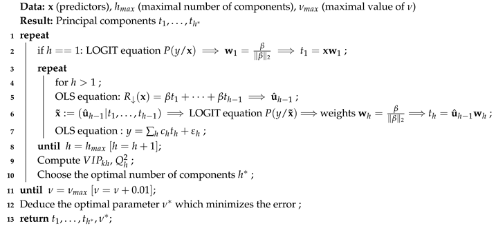
The first Gini-PLS algorithm was proposed by [11]. We describe below the new Gini-PLS algorithm based on the generalized co-Gini opetaror. The generalized Gini-PLS algorithm is depicted in Figure 4.

Step 1: A weight vector ${\mathbf{w}}_1$ is first built to improve the link (in the co-Gini sense) between the predicted variable y and the predictors $\mathbf{x}$:

$$max{\mathrm{cog}}_{\nu }(y,\mathbf{x}{\mathbf{w}}_1),\mathrm{s}.\mathrm{t}.{∥{\mathbf{w}}_1∥}_1=1.$$

The solution of this program is:

$${\mathbf{w}}_1=\frac{{\mathrm{cog}}_{\nu }(y,\mathbf{x})}{{∥{\mathrm{cog}}_{\nu }(y,\mathbf{x})∥}_1}.$$

As in the standard PLS case, the target y is regressed by OLS on the first component $t_1=\mathbf{x}{\mathbf{w}}_1$:

$$y={\widehat{c}}_1{t}_1+{\widehat{\epsilon }}_1.$$

Step 2: The rank vector of each regressor $R_{\downarrow }\left(x_k\right)$ is regressed by OLS on $t_1$ (with residuals ${\widehat{\mathbf{u}}}_1)$:

$$R_{\downarrow }\left(\mathbf{x}\right)=\widehat{\beta }{t}_1+{\widehat{\mathbf{u}}}_1.$$

The second component $t_2$ is given by:

$$max{\mathrm{cog}}_{\nu }({\widehat{\epsilon }}_1,{\widehat{\mathbf{u}}}_1{\mathbf{w}}_2)\mathrm{s}.\mathrm{t}.{∥{\mathbf{w}}_2∥}_1=1⟹{\mathbf{w}}_2=\frac{{\mathrm{cog}}_{\nu }({\widehat{\epsilon }}_1,{\widehat{\mathbf{u}}}_1)}{{∥{\mathrm{cog}}_{\nu }({\widehat{\epsilon }}_1,{\widehat{\mathbf{u}}}_1)∥}_1}⟹t_2={\widehat{\mathbf{u}}}_1{\mathbf{w}}_2.$$

Thereby, the components $t_1\perp t_2$ allow a link to be established between y and $\mathbf{x}$ by OLS:

$$y={\widehat{c}}_1{t}_1+{\widehat{c}}_2{t}_2+{\widehat{\epsilon }}_2.$$

Step h: Partial regressions are run up to $t_{h-1}$ :

$$R_{\downarrow }\left(\mathbf{x}\right)=\beta t_1+\cdots +\gamma t_{h-1}+{\widehat{\mathbf{u}}}_{h-1}.$$

Then, after maximization:

$${\mathbf{w}}_h=\frac{{\mathrm{cog}}_{\nu }({\widehat{\epsilon }}_{h-1},{\widehat{\mathbf{u}}}_{h-1})}{{∥{\mathrm{cog}}_{\nu }({\widehat{\epsilon }}_{h-1},{\widehat{\mathbf{u}}}_{h-1})∥}_1}⟹t_h={\widehat{\mathbf{u}}}_{h-1}{\mathbf{w}}_h,$$

we have by OLS,

$$y={\widehat{c}}_1{t}_1+\cdots +{\widehat{c}}_h{t}_h+{\epsilon }_h.$$

A cross validation makes it possible to find the optimal number of $h>1$ components to retain. To test for a component $t_h$, we compute the model prediction with h components including document d, ${\widehat{y}}_{h_d}$, and then without document d, ${\widehat{y}}_{h_{(-d)}}$. The operation is iterated for all d varying from 1 to N: each time we remove the observation d, we re-estimate the model. To measure the significance of the model, we measure the predicted residual sum of squared issued from the model with h components:

$$PRES{S}_h=\sum _{d=1}^N{\left(y_d-{\widehat{y}}_{h_{(-d)}}\right)}^2.$$

The sum of squared residuals of the model with $h-1$ components is:

$$RS{S}_{h-1}=\sum _{d=1}^N{\left(y_d-{\widehat{y}}_{{(h-1)}_d}\right)}^2.$$

The test statistics is:

$$Q_h^2=1-\frac{PRES{S}_h}{RS{S}_{h-1}}.$$

The component $t_h$ is retained in the analysis if $\sqrt{PRES{S}_h}\le 0.95\sqrt{RS{S}_h}$. In other terms, if $Q_h^2\ge 0.0975=(1-0.{95}^2)$, $t_h$ is significant in the sense that it improves the power of prediction of the model. In order to test for $t_1$, we use:

$$RS{S}_0=\sum _{d=1}^N{\left(y_d-\overline{y}\right)}^2.$$

As in the standard PLS regression, the $VI{P}_{hj}$ statistic is measured in order to select the word $x_j$ which has the most significant impact on the decision y. The most significant words are those including $VI{P}_{hj}>1$ with:

$$VI{P}_{hj}:=\sqrt{\frac{m{\sum }_{\ell =1}^{h}Rd(y;t_{\ell })w_{\ell j}^2}{Rd(y;t_1,\dots ,t_h)}}$$

and

$$Rd(y;t_1,\dots ,t_h):=\frac{1}{m}\sum _{\ell =1}^h{\mathrm{cor}}^2(y,t_{\ell })=:\sum _{\ell =1}^{h}Rd(y;t_{\ell }),$$

with ${\mathrm{cor}}^2(y,t_{\ell })$ being Pearson’s correlation between y and component $t_{\ell }$. This information is back propagated into the model (only once) in order to obtain the optimal number of components (on training data). The target variable y is then predicted as follows:

$$category\left(x\right)=\left\{\begin{array}{cc}0\hfill & \mathrm{if}\widehat{y}<0.5\hfill \\ 1\hfill & \mathrm{otherwise}.\hfill \end{array}\right.$$

Generalized LOGIT-Gini-PLS

As can be seen in the generalized Gini-PLS algorithm, the weights ${\mathbf{w}}_j$ come from the generalized co-Gini operator applied to a Boolean variable $y\in \{0,1\}$. In order to find the weights ${\mathbf{w}}_j$ which maximize the link between the words $x_j$ and the decision y, we propose to use the LOGIT regression—in other words, a sigmoid which is better adapted to Boolean variables. Thus, in each step of the Gini-PLS regression, we replace the maximization of the co-Gini by measuring the following conditional probability:

$$P(y_d=1/\mathbf{x}={\mathbf{x}}_d)=\frac{exp\left\{{\mathbf{x}}_d\beta \right\}}{1+exp\left\{{\mathbf{x}}_d\beta \right\}}$$

(LOGIT)

where ${\mathbf{x}}_d$ is the d-th line of the matrix $\mathbf{x}$ of the predictors (being the words in judgment d). The estimation of the vector $\beta$ is done by maximum likelihood. Therefore, at each step h of the PLS algorithm, the weights ${\mathbf{w}}_h$ are derived as follows:

$${\mathbf{w}}_h=\frac{\beta }{{\parallel \beta \parallel }_2}$$

The generalized LOGIT-Gini-PLS algorithm is depicted in Algorithm 1.

Algorithm 1: Generalized LOGIT-Gini-PLS (training).

5. Experiments and Results

We discuss the performance of various popular algorithms and the impact of data quantity and imbalance, heuristics, and explicit restriction of judgments to sections (regions) related to the claim category, as well as their ability to ignore other requests in the judgment. These experiments also aim to compare the effectiveness of LOGIT-Gini-PLS with other machine learning techniques. As in Im et al. [33], we compare different combinations of classification algorithms and term weighting methods (used for text representation). These combinations represent 600 experimental configurations including: (See https://github.com/tagnyngompe/taj-ginipls to enjoy the Python code of the Gini-PLS algorithms).

• 12 algorithms of classification: Naive Bayes (NB), Support Vector Machine (SVM), K-nearest neighbors (KNN), Linear and quadratic discriminant analysis (LDA/QDA), Tree, fastText, Naive Bayes SVM (NBSVM), generalized Gini-PLS (Gini-PLS), LOGIT-PLS [34], generalized LOGIT-Gini-PLS (LogitGiniPLS), and the usual PLS algorithm (StandardPLS);
• 11 global weighting schemes (cf. Table 5): ${\chi }^2$, $dbidf$, ${\Delta }_{DF}$, $dsidf$, $gss$, $idf$, $ig$, $mar$, $ngl$, $rf$, $av{g}_{global}$ (mean of the global metrics);
• 6 local weighting schemes (cf. Table 6): $tf$, $tp$, $logtf$, $atf$, $logave$, et $av{g}_{local}$ (mean of the local metrics).

5.1. Assessment Protocol

Two assessment metrics are used: precision and $F_1$-measure. To take into account the imbalance between the classes, the macro-average is preferred (As suggested by a reviewer, the MCC could be used for the data imbalance). It is the aggregation of the individual contribution of each class. It is calculated from the macro-averages of the precision ($P_{macro}$) and of the recall ($R_{macro}$), which are calculated according to the average numbers of true positives ($\overline{TP}$) , false positives ($\overline{FP}$), and false negatives ($\overline{FN}$) as follows: [35]: $P_{macro}=\frac{\overline{TP}}{\overline{TP}+\overline{FP}}$, $R_{macro}=\frac{\overline{TP}}{\overline{TP}+\overline{FN}}$.

The efficiency of algorithms often depends on the hyper-parameters for which optimal values must be determined. The scikit-learn [36] library implements two strategies for finding these values: RandomSearch and GridSearch. Despite the speed of the RandomSearch method, it is non-deterministic and the values it finds give a less accurate prediction than the default values. It is the same for the GridSearch method, which is very slow, and therefore impractical in view of the large number of configurations to be evaluated. Consequently, the values used for the experiments are the values defined by default (

Table 7. Values of the hyperparameters of the algorithms.

Algorithms	Hyperparameters
SVM	$C=1.0;\gamma =\frac{1}{\left|V\right|\times var\left(X\right)};kernel=RBF$
KNN	$k=5$
LDA	$solver=svd,n\_components=10$
QDA	no regularization of the covariance estimate
Tree	Gini criterion
NBSVM	n-grams of 1 to 3 words
Gini-PLS	$h_{max}=10$
Logit-PLS	$h_{max}=10$
Gini-Logit-PLS	$h_{max}=10;\nu =14$

).

5.2. Classification on the Basis of the Whole Judgment

By representing the entire judgment using various vector representations, the algorithms are compared with the representations that are optimal for them. We note from the results of

Table 8. Comparison of word representation and algorithms to detect the the judicial outcome.

Representation	Algorithm	${\mathit{F}}_1$	min	Cat. Min	Max	Cat. Max	$\mathbf{Best}\left({\mathit{F}}_1\right)$-${\mathit{F}}_1$	Max-Min	Rank
$tf-gss$	Tree	0.668	0.5	doris	0.92	dcppc	0	0.42	1
$tf-av{g}_{global}$	LogitPLS	0.648	0.518	danais	0.781	dcppc	0.02	0.263	13
$tf-av{g}_{global}$	StandardPLS	0.636	0.49	danais	0.836	dcppc	0.032	0.346	24
$tf-{\Delta }_{DF}$	GiniPLS	0.586	0.411	danais	0.837	dcppc	0.082	0.426	169
$tf-{\Delta }_{DF}$	LogitGiniPLS	0.578	0.225	styx	0.772	dcppc	0.09	0.547	220
-	NBSVM	0.494	0.4	styx	0.834	dcppc	0.174	0.434
-	fastText	0.412	0.343	doris	0.47	danais	0.256	0.127

that the trees are on average better for all the categories even if on average the $F_1$-measure is limited to 0.668. The results of PLS extensions are not very far from those of trees with differences of $F_1$-measure around 0.1 (if we choose the right representation scheme).

The $F_1$ average scores of the NBSVM and fastText algorithms generally do not exceed 0.5 despite being specially designed for texts. It can be noticed that they are very sensitive to the imbalance of data between the categories (more rejections than acceptances). Furthermore, it is more difficult to detect the acceptance of the requests. Indeed, these algorithms classify all the test data with the majority label (meaning) i.e., rejection, and therefore, they hardly detect some request acceptance. The case of the categories doris and dcppc for the NBSVM ($F_{1macro}=0.834$) tends to demonstrate the strong sensitivity to negative cases of these algorithms since the $F_1$-measure of “reject” is always higher than that of “accept” (

Table 9. Evaluation of fastText and NBSVM for detecting judicial outcomes for each claim category.

Cat.	Algo.	Prec.	Prec. equi.	err-0	err-1	${\mathit{F}}_1\left(0\right)$	${\mathit{F}}_1\left(1\right)$	${\mathit{F}}_{1\mathbf{macro}}$
dcppc	NBSVM	0.875	0.812	0	0.375	0.916	0.752	0.834
danais	fastText	0.888	0.5	0	1	0.941	0	0.47
danais	NBSVM	0.888	0.5	0	1	0.941	0	0.47
concdel	fastText	0.775	0.5	0	1	0.853	0	0.437
concdel	NBSVM	0.775	0.5	0	1	0.873	0	0.437
acpa	fastText	0.745	0.5	0	1	0.853	0	0.426
acpa	NBSVM	0.745	0.5	0	1	0.853	0	0.426
doris	NBSVM	0.5	0.492	0.167	0.85	0.63	0.174	0.402
dcppc	fastText	0.667	0.5	0	1	0.8	0	0.4
styx	fastText	0.667	0.5	0	1	0.8	0	0.4
styx	NBSVM	0.667	0.5	0	1	0.8	0	0.4
doris	fastText	0.523	0.5	0	1	0.686	0	0.343

0 == “reject” et 1 == “accept”; Cat.: Categories of claim; Algo. : algorithm; err-0: error rate of “reject”; err-1: error rate of “accept’; Prec.: global precision ($accuracy=\frac{TP}{N}$); Prec. equi.: $\frac{1}{2}(accuracy\left(0\right)+accuracy\left(1\right))$.

).

PLS algorithms systematically exceed the performance ($F_1$-measurement) of fastText and NBSVM from 10 to 20 points. This tends to demonstrate the effectiveness of PLS techniques in their role of reduction of dimensions. Gini-PLS algorithms do not operate any better than conventional PLS algorithms. Presumably, the reduction of dimensions is done while still retaining too much noise in the data. This is confirmed by the results of the trees which remain very mixed for which the $F_1$-measure (0.668) that exceeds barely that of Logit-PLS (0.648). It therefore seems necessary to proceed with zoning in the judgment to better identify relevant information and thereby reduce the noise.

5.3. Classification Based on Sections of Judgments Including the Vocabulary of the Category

Since the judgments are related to several categories of claim, we experiment with restrictions of the textual content based on different types of regions in judgments. The first types of regions are sections of the judgment: the description of facts and proceedings (Facts and Proceedings), judges’ reasoning to justify their decisions (Opinion), the summary of judges’ decisions (Holding). The sections are identified using a text labeling method [37]. Other types of regions are statements extracted from the sections related to the category of claim. They express either a claim, a result, a previous result (result_a), judges’ reasoning about the category (context). These statements are extracted using regular expressions and are used in the restriction only if they contain a key-phrase of the category. The region-vector representation-algorithm combinations are compared in

Table 10. Accuracy of the classification with restriction of judgments to specific regions.

Category	Region	Representation	Algorithm	${\mathit{F}}_1$
	claim_result_a_result_context	$tf-dbidf$	Tree	0.846
acpa	facts and proceedings_opinion_holding	$tf-dbidf$	StandardPLS	0.697
	facts and proceedings_opinion_holding	$tf-av{g}_{global}$	LogitPLS	0.683
	facts and proceedings_opinion_holding	$tf-gss$	Tree	0.798
concdel	opinion	$tf-idf$	LogitGiniPLS	0.703
	context	$logave-dbidf$	StandardPLS	0.657
	claim_result_a_result_context	$av{g}_{local}-{\chi }^2$	Tree	0.813
danais	claim_result_a_result_context	$atf-av{g}_{global}$	LogitPLS	0.721
	claim_result_a_result_context	$atf-av{g}_{global}$	StandardPLS	0.695
	claim_result_a_result_context	$tf-{\chi }^2$	Tree	0.985
dcppc	claim_result_a_result_context	$tf-{\chi }^2$	LogitPLS	0.94
	facts and proceedings_opinion_holding	$tp-mar$	StandardPLS	0.934
	facts and proceedings_opinion_holding	$tp-dsidf$	GiniPLS	0.806
doris	facts and proceedings_opinion_holding	$tp-dsidf$	LogitGiniPLS	0.806
	facts and proceedings_opinion_holding	$atf-ig$	StandardPLS	0.772
	opinion	$tf-dsidf$	Tree	1
styx	claim_result_a_result_context	$logave-dsidf$	LogitGiniPLS	0.917
	facts and proceedings_opinion_holding	$tf-rf$	GiniPLS	0.833

. The accuracy rate ($F_1$) increases significantly with the reduction of the judgment to regions, except for the doris category. The best restriction combines regions including the vocabulary of the category in the section Facts and Proceedings (request and previous result), in the Opinion section (context), and in the Holding section (result).

It is noteworthy that restricting the training of the model to the section facts and proceedings corresponds to the prediction of the judge’s outcome. When additional information is employed to train the model, such as opinion and holding, the task is reduced to an identification or an extraction of the judge’s outcome.

After reducing the size of the judgment, the trees provide excellent results, followed very closely by our GiniPLS and LogitGiniPLS algorithms. For example, in the dcppc category (see Table 5), Tree performance ($F_1$ = 0.985) slightly exceeds the LogitPLS (0.94) and standard PLS (0.934) algorithms. In the category concdel, Tree performance ($F_1$ = 0.798) is still closely followed by LogitGiniPLS (0.703) and standard PLS (0.657) algorithms.

The most interesting case is concerned with neighborhood disturbances (doris category). These judgments often involve multiple information that is sometimes difficult to synthesize, even for humans. The argumentation exposed in doris is related to multiple information (problems of views, sunshine, trees, etc.) so that the factual elements conditioning the identification of the judicial outcomes are sometimes complex. This information can be either under-represented or over-represented depending on the vectorization scheme. Our GiniPLS algorithm (like our LogitGiniPLS) seems to be particularly suitable for this category of request. The $F_1$-measures obtained in this category amount to 0.806 (for GiniPLS and LogitGiniPLS) and 0.772 for StandardPLS while the trees of decisions are not part of the relevant algorithms for this category of request (or among the best three algorithms). This result reinforces the idea that our GiniPLS algorithms can sometimes compete with decision trees that act as a benchmark in the literature dealing with small datasets. This result would make it possible in the future to consider including our GiniPLS algorithms in ensemble methods to broaden the spectrum of algorithms robust to outliers and which at the same time play a role of data compression.

6. Conclusions

This article attempted to simplify the extraction of the meaning of the result rendered by the judges on a request for a given category of claims. It consisted in formulating the problem as a task of judgments’ binary classification. Ten classification algorithms were tested over 55 methods of vector embeddings. We observed that the classification results were mainly influenced by three characteristics of our data. First, the very small number of training examples disadvantaged certain algorithms (sensitivity to outliers), such as fastText, which requires several thousand examples to update its parameters. Second, the strong imbalance between the classes (“accept” vs. “reject”) made it difficult to recognize the minority class which is generally the “accept” class. This was shown by the strong gap between the errors on “reject” and those on “accept”, as well as the good results obtained on dcppc. Finally, the presence of other claim categories in the judgment degraded the efficiency of the classification because the algorithms did not manage alone to find the elements in a direct relation with the analyzed category. This was demonstrated by the positive impact of the restriction of the content to be classified in certain particular regions of the decision, even if the appropriate restrictions depended on the category.

Decision trees were suitable for the classification task, but the use of Gini-PLS and Gini-Logit-PLS made it possible to obtain performances fairly close to those of trees and sometimes higher. It would be interesting to combine these variants of PLS algorithms, with others such as Sparse-PLS which could perhaps help to solve the problem of sparse vectors. There is also a large number of neural architectures for the classification of judgment and very large numbers of weighting metrics for the representation of texts, but none seem to fit all categories. Therefore, a study on the use of semantic embedding representations like Sent2Vec [38] or Doc2Vec [39] would be interesting.

References

1. Chalkidis, I.; Androutsopoulos, I. A Deep Learning Approach to Contract Element Extraction; JURIX: Luxembourg, 2017; pp. 155–164. [Google Scholar]
2. Wei, F.; Qin, H.; Ye, S.; Zhao, H. Empirical study of deep learning for text classification in legal document review. In Proceedings of the 2018 IEEE International Conference on Big Data (Big Data), Seattle, WA, USA, 10–13 December 2018; pp. 3317–3320. [Google Scholar]
3. Luo, B.; Feng, Y.; Xu, J.; Zhang, X.; Zhao, D. Learning to Predict Charges for Criminal Cases with Legal Basis. In Proceedings of the 2017 Conference on Empirical Methods in Natural Language Processing, Copenhagen, Denmark, 7–11 September 2017; pp. 2727–2736. [Google Scholar]
4. Zhong, H.; Guo, Z.; Tu, C.; Xiao, C.; Liu, Z.; Sun, M. Legal Judgment Prediction via Topological Learning; EMNLP: Brussels, Belgium, 2018; pp. 350–354. [Google Scholar]
5. Long, S.; Tu, C.; Liu, Z.; Sun, M. Automatic judgment prediction via legal reading comprehension. In Proceedings of the 18th China National Conference, Kunming, China, 18–20 October 2019; pp. 558–572. [Google Scholar]
6. Guo, X.; Zhang, H.; Ye, L.; Li, S. RnRTD: Intelligent Approach Based on the Relationship-Driven Neural Network and Restricted Tensor Decomposition for Multiple Accusation Judgment in Legal Cases. Comput. Intell. Neurosci. 2019, 2019, 6705405. [Google Scholar] [CrossRef] [PubMed]
7. Chalkidis, I.; Androutsopoulos, I.; Aletras, N. Neural legal judgment prediction in english. arXiv 2019, arXiv:1906.02059. [Google Scholar]
8. O’Sullivan, C.; Beel, J. Predicting the Outcome of Judicial Decisions made by the European Court of Human Rights. In Proceedings of the 27th AIAI Irish Conference on Artificial Intelligence and Cognitive Science, Dublin, Ireland, 6–7 December 2018. [Google Scholar]
9. Lage-Freitas, A.; Allende-Cid, H.; Santana, O.; de Oliveira-Lage, L. Predicting Brazilian court decisions. arXiv 2018, arXiv:1905.10348. [Google Scholar]
10. Tagny Ngomp, G. Mthodes Danalyse Smantique de Corpus de Dcisions Jurisprudentielles. Ph.D. Thesis, IMT Mines Ales, Ales, France, 2020. [Google Scholar]
11. Mussard, S.; Souissi-Benrejab, F. Gini-PLS Regressions. J. Quant. Econ. 2018, 1–36. [Google Scholar] [CrossRef]
12. Salton, G.; Buckley, C. Term-weighting Approaches In Automatic Text Retrieval. Inf. Process. Manag. 1988, 24, 513–523. [Google Scholar] [CrossRef] [Green Version]
13. Sparck Jones, K. A statistical interpretation of term specificity and its application in retrieval. J. Doc. 1972, 28, 11–21. [Google Scholar] [CrossRef]
14. Wu, H.; Salton, G. A comparison of search term weighting: Term relevance vs. inverse document frequency. In Proceedings of the 4th Annual International ACM SIGIR Conference on Information Storage and Retrieval: Theoretical Issues in Information Retrieval; ACM: New York, NY, USA, 1981; Volume 16, pp. 30–39. [Google Scholar]
15. Jones, K.S.; Walker, S.; Robertson, S.E. A Probabilistic Model Of Information Retrieval: Development And Comparative Experiments. Inf. Process. Manag. 2000, 36, 809–840. [Google Scholar] [CrossRef]
16. Yang, Y.; Pedersen, J.O. A Comparative Study on Feature Selection in Text Categorization; ICML: Broken Arrow, OK, USA, 1997; Volume 97, pp. 412–420. [Google Scholar]
17. Lan, M.; Tan, C.L.; Su, J.; Lu, Y. Supervised and traditional term weighting methods for automatic text categorization. IEEE Trans. Pattern Anal. Mach. Intell. 2009, 31, 721–735. [Google Scholar] [CrossRef] [PubMed]
18. Schütze, H.; Hull, D.A.; Pedersen, J.O. A comparison of classifiers and document representations for the routing problem. In Proceedings of the 18th Annual International ACM SIGIR Conference on Research and Development in Information Retrieval, Seattle, WA, USA, 9–13 July 1995; pp. 229–237. [Google Scholar]
19. Ng, H.T.; Goh, W.B.; Low, K.L. Feature selection, perceptron learning, and a usability case study for text categorization. In Proceedings of the 20th Annual International ACM SIGIR Conference on Research and Development in Information Retrieval, Philadelphia, PA, USA, 27–31 July 1997; ACM: New York, NY, USA, 1997; Volume 31, pp. 67–73. [Google Scholar]
20. Galavotti, L.; Sebastiani, F.; Simi, M. Experiments on the use of feature selection and negative evidence in automated text categorization. In Proceedings of the International Conference on Theory and Practice of Digital Libraries, Lisbon, Portugal, 18–20 September 2020; Springer: Berlin/Heidelberg, Germany, 2000; pp. 59–68. [Google Scholar]
21. Marascuilo, L.A. Large-sample multiple comparisons. Psychol. Bull. 1966, 65, 280. [Google Scholar] [CrossRef] [PubMed]
22. Paltoglou, G.; Thelwall, M. A study of information retrieval weighting schemes for sentiment analysis. In Proceedings of the 48th Annual Meeting of the Association for Computational Linguistics, Uppsala, Sweden, 11–16 July 2010; Association for Computational Linguistics: Stroudsburg, PA, USA, 2010; pp. 1386–1395. [Google Scholar]
23. Manning, C.D.; Raghavan, P.; Schütze, H. Scoring, term weighting and the vector space model. In Introduction to Information Retrieval; Cambridge University Press: Cambridge, UK, 2009; Chapter 6; pp. 109–133. [Google Scholar]
24. Wold, H. Estimation of Principal Components and Related Models by Iterative Least Squares; Multivar. Anal. Academic Press: Cambridge, MA, USA, 1966; pp. 391–420. [Google Scholar]
25. Lacroux, A. Les avantages et les limites de la méthode «Partial Least Square»(PLS): Une illustration empirique dans le domaine de la GRH. Rev. Gest. Ressour. Hum. 2011, 80, 45–64. [Google Scholar] [CrossRef]
26. Kroll, C.N.; Song, P. Impact of multicollinearity on small sample hydrologic regression models. Water Resour. Res. 2013, 49, 3756–3769. [Google Scholar] [CrossRef]
27. Liu, Y.; Rayens, W. PLS and dimension reduction for classification. Comput. Stat. 2007, 22, 189–208. [Google Scholar] [CrossRef]
28. Durif, G.; Modolo, L.; Michaelsson, J.; Mold, J.E.; Lambert-Lacroix, S.; Picard, F. High dimensional classification with combined adaptive sparse PLS and logistic regression. Bioinformatics 2017, 34, 485–493. [Google Scholar] [CrossRef] [PubMed]
29. Bazzoli, C.; Lambert-Lacroix, S. Classification based on extensions of LS-PLS using logistic regression: Application to clinical and multiple genomic data. BMC Bioinform. 2018, 19, 314. [Google Scholar] [CrossRef] [PubMed]
30. Zeng, X.Q.; Wang, M.W.; Nie, J.Y. Text classification based on partial least square analysis. In Proceedings of the 2007 ACM Symposium on Applied Computing, Seoul, Korea, 11–15 March 2007; pp. 834–838. [Google Scholar]
31. Schechtman, E.; Yitzhaki, S. A family of correlation coefficients based on the extended Gini index. J. Econ. Inequal. 2003, 1, 129–146. [Google Scholar] [CrossRef]
32. Olkin, I.; Yitzhaki, S. Gini regression analysis. Int. Stat. Rev./Rev. Int. Stat. 1992, 60, 185–196. [Google Scholar] [CrossRef]
33. Im, C.J.; Kim, D.W.; Mandl, T. Text Classification for Patents: Experiments with Unigrams, Bigrams and Different Weighting Methods. Int. J. Contents 2017, 13, 66–74. [Google Scholar] [CrossRef]
34. Tenenhaus, M. La regression logistique PLS. In Modles Statistiques Pour Donnes Qualitatives; Droesbeke, J.-J., Lejeune, M., Saporta, G., Eds.; Editions Technip: Paris, France, 2005; Chapter 12; pp. 263–276. [Google Scholar]
35. Van Asch, V. Macro- and Micro-Averaged Evaluation Measures; Technical Report; Computational Linguistics & Psycholinguistics (CLiPS): Antwerpen, Belgium, 2013. [Google Scholar]
36. Pedregosa, F.; Varoquaux, G.; Gramfort, A.; Michel, V. Scikit-learn: Machine Learning in Python. J. Mach. Learn. Res. 2011, 12, 2825–2830. [Google Scholar]
37. Tagny Ngompé, G.; Harispe, S.; Zambrano, G.; Montmain, J.; Mussard, S. Detecting Sections and Entities in Court Decisions Using HMM and CRF Graphical Models. In Advances in Knowledge Discovery and Management: Volume 8; Pinaud, B., Guillet, F., Gandon, F., Largeron, C., Eds.; Springer International Publishing: Berlin/Heidelberg, Germany, 2019; pp. 61–86. [Google Scholar] [CrossRef]
38. Pagliardini, M.; Gupta, P.; Jaggi, M. Unsupervised Learning of Sentence Embeddings using Compositional n-Gram Features. In Proceedings of the NAACL 2018 Conference of the North American Chapter of the Association for Computational Linguistics, New Orleans, LA, USA, 1–6 June 2018. [Google Scholar]
39. Le, Q.; Mikolov, T. Distributed representations of sentences and documents. In Proceedings of the International Conference on Machine Learning, Beijing, China, 21–26 June 2014; pp. 1188–1196. [Google Scholar]
Figure 1. Number of claims in judgments.
Stats 03 00027 g001
Figure 2. Distribution of judges’ decisions within each category of claims.
Stats 03 00027 g002
Figure 3. Distribution of the size of the decision by tokens.
Stats 03 00027 g003
Figure 4. Generalized Gini-PLS algorithm.
Stats 03 00027 g004