L_p Loss Functions in Invariance Alignment and Haberman Linking with Few or Many Groups

Abstract

The comparison of group means in latent variable models plays a vital role in empirical research in the social sciences. The present article discusses an extension of invariance alignment and Haberman linking by choosing the robust power loss function $\rho \left(x\right)={\left|x\right|}^p$$(p>0)$. This power loss function with power values p smaller than one is particularly suited for item responses that are generated under partial invariance. For a general class of linking functions, asymptotic normality of estimates is shown. Moreover, the theory of M-estimation is applied for obtaining linking errors (i.e., inference with respect to a population of items) for this class of linking functions. In a simulation study, it is shown that invariance alignment and Haberman linking have comparable performance, and in some conditions, the newly proposed robust Haberman linking outperforms invariance alignment. In three examples, the influence of the choice of a particular linking function on the estimation of group means is demonstrated. It is concluded that the choice of the loss function in linking is related to structural assumptions about the pattern of noninvariance in item parameters.

1. Introduction

In the comparison of multiple groups in latent variable models like factor analysis or item response models, some identifying assumptions have to be posed. In practice, it is often assumed that item parameters are equal across groups, which is denoted as invariance. The invariance concept has been very prominent in psychology and the social sciences in general [1,2]. For example, in international large-scale assessment studies in education like the programme for international student assessment (PISA), the necessity of invariance is strongly emphasized [3].

In the violation of invariance, linking approaches have been proposed to allow group comparisons. In this article, two important linking approaches are compared: invariance alignment [4] and Haberman linking [5]. These two approaches are contrasted by introducing a unifying notation. Moreover, these approaches are extended by considering a broad family of linking functions, the $L_p$ loss function. By means of this extension, invariance alignment and Haberman linking appear to be very similar on a formal level, and through a simulation study, it is shown that they provide comparable results.

The article is structured as follows. In Section 2, unidimensional factor models are introduced. In Section 3, the theory of the proposed extension of invariance alignment and Haberman linking is described. In Section 4, asymptotic results for general linking functions that also (partly) apply to invariance alignment and Haberman linking are presented. In Section 5, two simulation studies targeting the case of continuous or dichotomous items, respectively, are presented. In Section 6, the usefulness of the linking approaches is demonstrated throughs three empirical examples. Finally, Section 7 concludes with a discussion.

2. Unidimensional Factor Model with Partial Invariance

In this section, the unidimensional factor model for continuous and dichotomous items for multiple groups (i.e., multiple populations) is introduced. Afterward, different assumptions about levels of invariance of item parameters are discussed.

2.1. Unidimensional Factor Model

Let $X_{ig}$ denote the item response variable of item i $(i=1,\dots ,I)$ in group g$(g=1,\dots ,G)$. In Section 2.1.1, we discuss the unidimensional factor model for continuous items. In Section 2.1.2, the factor model for dichotomous items is introduced.

2.1.1. Continuous Items

For continuous items $X_{ig}$, a unidimensional factor model is assumed [6]

$$X_{ig}={\nu }_{ig}+{\lambda }_{ig}{\theta }_g+{\epsilon }_{ig},{\theta }_g\sim N({\mu }_g,{\sigma }_g^2),{\epsilon }_{ig}\sim N(0,{\omega }_{ig}),$$

(1)

where ${\lambda }_{ig}$ are item loadings (that are typically assumed to be nonnegative), and ${\nu }_{ig}$ are item intercepts. It has to be noted that the parameters in Equation (1) are not identified. An identified model is obtained by assuming a standardized latent variable ${\theta }_g$:

$$X_{ig}={\nu }_{ig,0}+{\lambda }_{ig,0}{\theta }_g+{\epsilon }_{ig},{\theta }_g\sim N(0,1),{\epsilon }_{ig}\sim N(0,{\omega }_{ig})$$

(2)

The model parameters are then related as follows

$${\lambda }_{ig,0}={\lambda }_{ig}{\sigma }_g$$

(3)

$${\nu }_{ig,0}={\nu }_{ig}+{\lambda }_{ig}{\mu }_g={\nu }_{ig}+\frac{{\lambda }_{ig,0}}{{\sigma }_g}{\mu }_g$$

(4)

The special case in which all loadings are set equal to 1 is referred to as the so-called tau-equivalent measurement model [7]. Only item intercepts have to be linked in this case.

2.1.2. Dichotomous Items

For dichotomous (i.e., binary) variables, a logistic link function $\mathrm{L}$ is employed, and the resulting unidimensional factor model is

$$P(X_{ig}=1|{\theta }_g)=\mathrm{L}({\nu }_{ig}+{\lambda }_{ig}{\theta }_g),{\theta }_g\sim N({\mu }_g,{\sigma }_g^2)$$

(5)

This model is also known as the two-parameter logistic (2PL) model [8] and is widely spread in the literature of item response theory (IRT) models, for example, [9,10]. One might view the IRT approach in Equation (5) as a special case of structural equation modeling (see Equation (1) for continuous items using the normal distribution assumption), employing the logistic link function [11].

Again, the model in Equation (5) is not identified, but an identified parameterization can be employed using the same conversion Formulas (3) and (4). It should be noted that the 2PL model in Equation (5) is often reparameterized as $P(X_{ig}=1|{\theta }_g)=\mathrm{L}\left({\lambda }_{ig}({\theta }_g-{\beta }_{ig})\right)$, where ${\beta }_{ig}=-{\nu }_{ig}/{\lambda }_{ig}$ are item difficulties. Using identified parameters ${\lambda }_{ig,0}$ and ${\beta }_{ig,0}$, the relations among item parameters hold by rewriting Equations (3) and (4)

$$log{\lambda }_{ig,0}=log{\lambda }_{ig}+log{\sigma }_g$$

(6)

$${\sigma }_g{\beta }_{ig,0}={\beta }_{ig}-{\mu }_g.$$

(7)

Equation (7) can also be rephrased in terms of random intercepts ${\nu }_{ig}$:

$${\sigma }_g\frac{{\nu }_{ig,0}}{{\lambda }_{ig,0}}=-{\beta }_{ig}+{\mu }_g.$$

(8)

The special case in which all item loadings ${\lambda }_{ig}$ are set to 1 is referred to as the one-parameter logistic model (1PL; a.k.a. the Rasch model; [12]). In this case, only item intercepts have to be linked. There is no need to distinguish linking based on item intercepts from linking based on item difficulties because it holds that ${\beta }_{ig}=-{\nu }_{ig}$.

2.2. Full Invariance, Partial Invariance, and Linking Methods

The main goal is to compare the distribution of ${\theta }_g$ among groups. As the unidimensional factor model is not identified, some identification constraints have to be imposed to enable group comparisons. Three main approaches can be distinguished that differ concerning the assumptions of item parameters.

First, in a full invariance approach [1,2,13,14] it is assumed that all item parameters are equal among groups, for example, ${\lambda }_{i1}=\dots ={\lambda }_{iG}$ and ${\nu }_{i1}=\dots ={\nu }_{iG}$ for all items $i=1,\dots ,I$. This approach presumes the existence of common item parameters ${\lambda }_i$ and ${\nu }_i$ across groups and the unidimensional factor model is identified by posing constraints on the parameters of the first group (i.e., ${\mu }_1=0$ and ${\sigma }_1=1$).

Second, in a partial invariance approach [15,16,17], it is assumed that a subset of item parameters is the same across groups. More formally, the group-specific item parameters are decomposed into common item parameters and group-specific item parameters as follows:

$${\lambda }_{ig}={\lambda }_i+u_{ig}\mathrm{and}{\nu }_{ig}={\nu }_i+e_{ig}$$

(9)

The existence of group-specific item parameters is also labeled as differential item functioning (DIF, [1,18]). The presence of group-specific item intercepts is denoted as uniform DIF, while the presence of group-specific item loadings is denoted as nonuniform DIF [18]. In partial invariance, it is assumed that a subset of effects $u_{ig}$ and $e_{ig}$ is equal to zero. In the extreme case that all parameters equal zero, full invariance is obtained. A crucial issue is that a researcher does not know which item parameters differ among groups and some statistical procedure has to be applied for detecting the group-specific parameters (see [19,20,21,22,23] for overviews). By assuming some zero effects $u_{ig}$ and $e_{ig}$ and the identification constraint ${\mu }_1=0$ and ${\sigma }_1=1$ of distribution parameters of the first group, the unidimensional factor model can be identified. In [24], it is suggested that at most $25\%$ of all item parameters can be noninvariant to get trustworthy estimates of group means in the IA approach, a rule that can be also transferred to the partial invariance approach (see also [25]).

Third, in a full noninvariance approach, all item parameters are allowed to differ among groups. The unidimensional factor model is identified by posing some identification constraints on group-specific parameters [26]. For example, ${\prod }_{i=1}^I{\lambda }_{ig}=1$ and ${\sum }_{i=1}^I{\nu }_{ig}=0$ (for all groups $g=1,\dots ,G$) are sufficient conditions for ensuring identifiability. In the linking approach see [27,28,29,30,31], the sets of identified group-specific item parameters ${\widehat{\mathit{\lambda }}}_{g,0}=({\widehat{\lambda }}_{1g,0},\dots ,{\widehat{\lambda }}_{Ig,0})$ and ${\widehat{\mathit{\nu }}}_{g,0}=({\widehat{\nu }}_{1g,0},\dots ,{\widehat{\nu }}_{Ig,0})$$(g=1,\dots ,G)$ are used to compute group means $\mathit{\mu }=({\mu }_1,\dots ,{\mu }_G)$ and group standard deviations $\mathit{\sigma }=({\sigma }_1,\dots ,{\sigma }_G)$ by minimizing some linking function $H(\mathit{\mu },\mathit{\sigma })=f(\mathit{\mu },\mathit{\sigma };{\widehat{\mathit{\lambda }}}_{1,0},\dots ,{\widehat{\mathit{\lambda }}}_{G,0},{\widehat{\mathit{\nu }}}_{1,0},\dots ,{\widehat{\mathit{\nu }}}_{G,0})$. The main idea is that deviations ${\lambda }_{ig}-{\lambda }_{ih}$ and ${\nu }_{ig}-{\nu }_{ih}$ should be small for all pairs of groups g and h. In this article, two linking methods will be investigated in more detail that are introduced in Section 3.

In practice, the full invariance or the partial invariance assumption are often only approximately fulfilled, and diversity of statistical methods has been proposed to tackle this case [32,33,34,35,36,37,38]. These approaches are of particular importance in studies of cross-cultural comparisons in which many groups (i.e., countries in this case) are involved [3,39]. Moreover, the issue of invariance is also vital in studies involving longitudinal measurements [40,41].

3. Linking Methods

In this section, the linking methods invariance alignment [4] and Haberman linking [5] are introduced. It was highlighted by researcher Matthias von Davier that the alignment method appears to be very similar to the Haberman linking approach (see [42], p. 4). In the following section, both approaches are discussed using a unifying notation.

3.1. Invariance Alignment

Asparouhov and Muthén [4,24] proposed the method of invariance alignment (IA) to define a linking method that maximizes the extent of invariant item parameters. IA is also labeled as alignment optimization [43,44].

The IA approach uses estimated identifiable item parameters ${\widehat{\lambda }}_{ig,0}$ and ${\widehat{\nu }}_{ig,0}$ ($i=1,\dots ,I$; $g=1,\dots ,G$) as the input. These parameters can be obtained from fitting a unidimensional factor model for continuous items or a unidimensional item response model for dichotomous items. The goal is to minimize deviations ${\lambda }_{ig}-{\lambda }_{ih}$ and ${\nu }_{ig}-{\nu }_{ih}$ for pairs of groups g and h. By rewriting Equations (3) and (4), we obtain

$${\lambda }_{ig}-{\lambda }_{ih}=\frac{{\lambda }_{ig,0}}{{\sigma }_g}-\frac{{\lambda }_{ih,0}}{{\sigma }_h}$$

(10)

$${\nu }_{ig}-{\nu }_{ih}={\nu }_{ig,0}-{\nu }_{ih,0}-{\lambda }_{ig,0}\frac{{\mu }_g}{{\sigma }_g}+{\lambda }_{ih,0}\frac{{\mu }_h}{{\sigma }_h}$$

(11)

These relations motivate the minimization of the following linking function for determining group means $\mathit{\mu }$ and standard deviations $\mathit{\sigma }$:

$$H(\mathit{\mu },\mathit{\sigma })=\sum _{i=1}^I\sum _{g,h=1}^G{w}_{i1,gh}\rho \left(\frac{{\widehat{\lambda }}_{ig,0}}{{\sigma }_g}-\frac{{\widehat{\lambda }}_{ih,0}}{{\sigma }_h}\right)+\sum _{i=1}^I\sum _{g,h=1}^G{w}_{i2,gh}\rho \left({\widehat{\nu }}_{ig,0}-{\widehat{\nu }}_{ih,0}-{\widehat{\lambda }}_{ig,0}\frac{{\mu }_g}{{\sigma }_g}+{\widehat{\lambda }}_{ih,0}\frac{{\mu }_h}{{\sigma }_h}\right)$$

(12)

where $w_{i1,gh}$ and $w_{i2,gh}$ are user-defined weights and $\rho$ is a loss function [45]. Asparouhov and Muthén [4,24] proposed to use $w_{i1,gh}=w_{i2,gh}=\sqrt{n_g{n}_h}$ and $\rho \left(x\right)=\sqrt{\left|x\right|}$. In this article, we propose the robust loss function $\rho \left(x\right)={\left|x\right|}^p$ for nonnegative p ($L_p$ loss function; [46,47,48,49,50]). To balance the impact of groups in the estimation, all weights $w_{i1,gh}$ and $w_{i2,gh}$ in Equation (12) could be chosen equal to 1. In the following, we omit weights for ease of notation.

3.1.1. A Reformulation as a Two-Step Minimization Problem

It is instructive to reformulate the minimization problem of H in Equation (12) as a two-step minimization problem. In the first step, the vector of group standard deviations $\mathit{\sigma }$ is obtained by minimizing

$$H_{1u}\left(\mathit{\sigma }\right)=\sum _{i=1}^I\sum _{g,h=1}^G\rho \left(\frac{{\widehat{\lambda }}_{ig,0}}{{\sigma }_g}-\frac{{\widehat{\lambda }}_{ih,0}}{{\sigma }_h}\right)$$

(13)

In the second step, estimated standard deviations ${\widehat{\sigma }}_g$ ($g=1,\dots ,G$) from the first step are used, and the vector of group means $\mathit{\mu }$ is obtained by minimizing the following criterion:

$$H_{2i}\left(\mathit{\mu }\right)=\sum _{i=1}^I\sum _{g,h=1}^G\rho \left({\widehat{\nu }}_{ig,0}-{\widehat{\nu }}_{ih,0}-{\widehat{\lambda }}_{ig}\frac{{\mu }_g}{{\widehat{\sigma }}_g}+{\widehat{\lambda }}_{ih}\frac{{\mu }_h}{{\widehat{\sigma }}_h}\right)$$

(14)

Alternatively, one can use relations (6) and (8) to define a linking function. We obtain

$$log{\lambda }_{ig}-log{\lambda }_{ih}=log{\lambda }_{ig,0}-log{\lambda }_{ih,0}-log{\sigma }_g+log{\sigma }_h$$

(15)

$${\beta }_{ig}-{\beta }_{ih}={\sigma }_g\frac{{\nu }_{ig,0}}{{\lambda }_{ig,0}}-{\sigma }_h\frac{{\nu }_{ih,0}}{{\lambda }_{ih,0}}+{\mu }_g-{\mu }_h$$

(16)

For estimating group standard deviations in the first step, logarithmized item loadings can be used by minimizing

$$H_{1l}\left(\mathit{\sigma }\right)=\sum _{i=1}^I\sum _{g,h=1}^G\rho \left(log{\widehat{\lambda }}_{ig,0}-log{\widehat{\lambda }}_{ih,0}+log{\sigma }_g-log{\sigma }_h\right)$$

(17)

For estimating group means in the second step, the differences in item difficulties in Equation (16) are used to minimize

$$H_{2d}\left(\mathit{\mu }\right)=\sum _{i=1}^I\sum _{g,h=1}^G\rho \left({\widehat{\sigma }}_g\frac{{\widehat{\nu }}_{ig,0}}{{\widehat{\lambda }}_{ig,0}}-{\widehat{\sigma }}_h\frac{{\widehat{\nu }}_{ih,0}}{{\widehat{\lambda }}_{ih,0}}+{\mu }_g-{\mu }_h\right)$$

(18)

The IA approach can be applied by combining the two alternatives of minimization functions for untransformed item loadings ($H_{1u}$) or logarithmized loadings ($H_{1l}$) and item intercepts ($H_{2i}$) or item difficulties ($H_{2d}$) for standard deviations and means, respectively. Hence, four different linking functions can be defined: $H_{1u}$ and $H_{2i}$ (Method IA1), $H_{1l}$ and $H_{2i}$ (Method IA2), $H_{1u}$ and $H_{2d}$ (Method IA3), and $H_{1l}$ and $H_{2d}$ (Method IA4). In this article, it is investigated in two simulation studies which linking method is to preferred with respect to the performance in the estimated group means $\widehat{\mathit{\mu }}$.

If loadings are set to 1 in the estimation (i.e., one-parameter models are used), the linking function only involves group means $\mathit{\mu }$ and item intercepts are linked. Then, the linking function (18) simplifies to

$$H_{2d}\left(\mathit{\mu }\right)=\sum _{i=1}^I\sum _{g,h=1}^G\rho \left({\widehat{\nu }}_{ig,0}-{\widehat{\nu }}_{ih,0}+{\mu }_g-{\mu }_h\right).$$

(19)

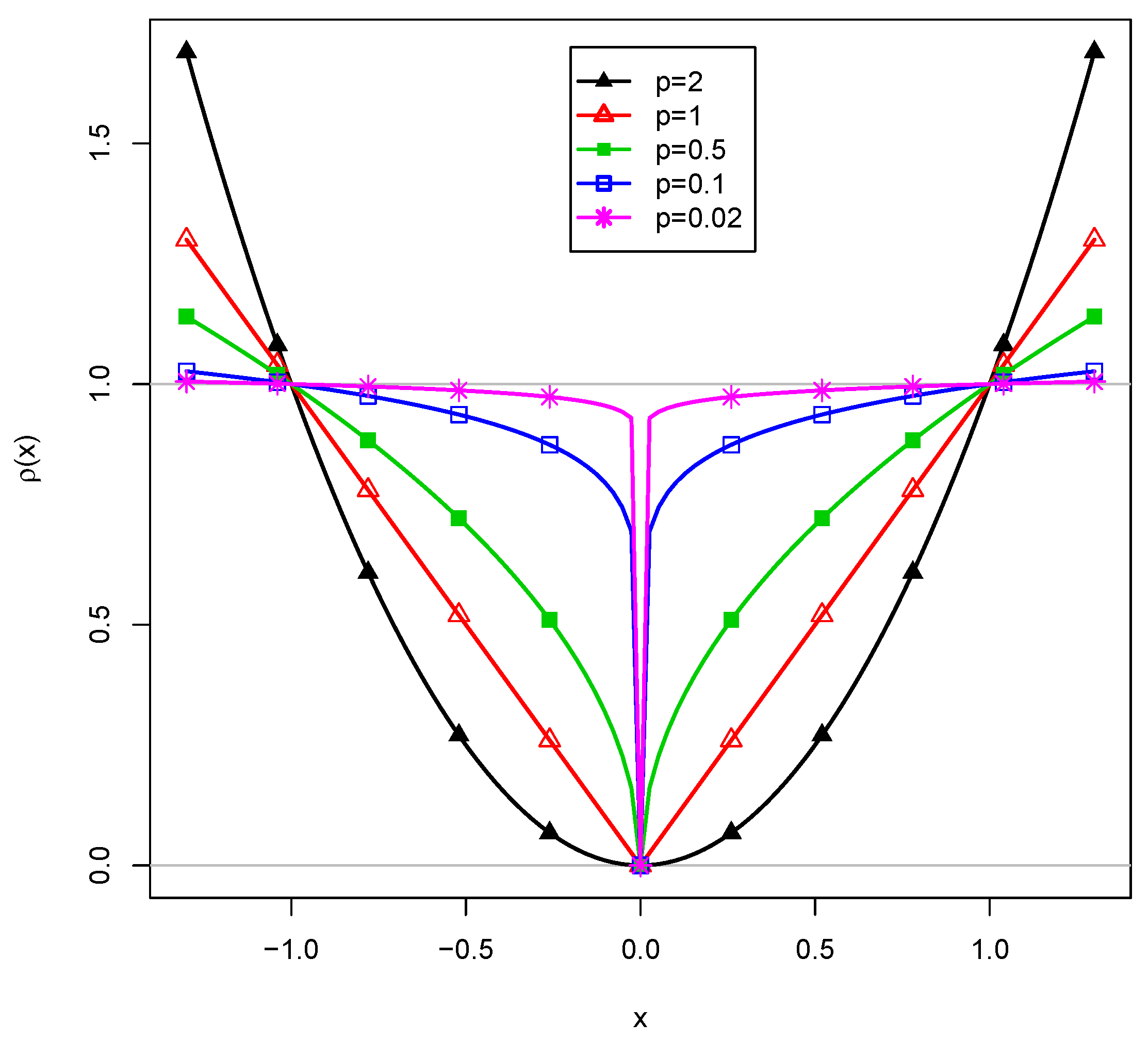
3.1.2. Choice of the Loss Function $\rho$

The statistical properties of the estimator for $\mathit{\mu }$ and $\mathit{\sigma }$ also strongly depend on the choice of the loss function $\rho$. In the case of partial invariance, only a few of the pairwise differences of item parameters are nonzero. This motivates the use of robust loss functions $\rho$ that are obtained with $p\le 1$ because a few large differences between group-specific item parameters can be interpreted as outlying cases [51,52,53,54,55,56,57,58,59]. Asparouhov and Muthén [4,24] implemented the loss function $\rho \left(x\right)=\sqrt{\left|x\right|}={\left|x\right|}^{0.5}$ in their commercial Mplus software [60]. The more general loss function $\rho \left(x\right)={\left|x\right|}^p$ is implemented in the R package sirt (see the function invariance.alignment; [61]). In Figure 1, the loss function $\rho$ is displayed for different values of p.

The case of the loss function can be motivated in the case of $G=2$ groups and the one-parameter model. In this case, only the mean ${\mu }_2$ of the second group has to be estimated and Equation (19) further simplifies to

$$H_{2d}\left({\mu }_2\right)=\sum _{i=1}^I{\left|{\widehat{\nu }}_{i1,0}-{\widehat{\nu }}_{i2,0}-{\mu }_2\right|}^p.$$

(20)

By inspecting Equation (20), it becomes clear that a generalized mean ${\mu }_2$ in an $L_p$ norm is estimated [62]. For $p=2$, it corresponds to the ordinary mean of observations ${\widehat{\delta }}_i={\widehat{\nu }}_{i1,0}-{\widehat{\nu }}_{i2,0}$. In this case, linking is also known as mean-mean linking [28]. With $p=1$, the $L_p$ mean is estimated as the median of observations ${\widehat{\delta }}_i$ (uniqueness presupposed). The case $p=0$ corresponds to the estimation of the mode of observations. Values between these three integers can be interpreted as intermediate cases. It should be noted that in the limiting case of $p=0$, the number of noninvariant item parameters is minimized because for $p=0$, Equation (20) reduces to

$$H_{2d}\left({\mu }_2\right)=\sum _{i=1}^I{\mathbf{1}}_{\{{\mu }_2={\widehat{\nu }}_{i1,0}-{\widehat{\nu }}_{i2,0}\}},$$

(21)

where $\mathbf{1}$ denotes the indicator function of a set.

3.1.3. Estimation

The loss function $\rho \left(x\right)={\left|x\right|}^p$ is not differentiable for $p\le 1$ that prevent from using optimization algorithms that rely on derivatives. However, in the alignment, the function $\rho$ is replaced by a differentiable approximating function ${\rho }_D\left(x\right)={(x^2+\epsilon )}^{p/2}$ using a small $\epsilon >0$ (e.g., $\epsilon =0.01$ that is used in the software Mplus, or $\epsilon =0.001$). Because ${\rho }_D$ is differentiable, quasi-Newton minimization approaches can be used that are implemented in standard optimizers in R (e.g., optim or nlmnib; [63]). For $p=0$, $\rho \left(x\right)$ is a step function that takes the value 0 for $x=0$ and 1 otherwise (see $p=0.02$ in Figure 1). In this case, the maximum approximation error by using ${\rho }_D$ is 1. For $p>0$, $\rho$ is a continuous function of x. The maximum difference is given as $|{\rho }_D\left(x\right)-\rho \left(x\right)|\le {\rho }_D\left(0\right)={\epsilon }^{p/2}$. For $p=0.02$ and $\epsilon =0.001$, it is 0.940. However, it strongly reduces to 0.039 for $x=0.005$. Also note that for empirical data, it is unlikely that exact values of 0 are obtained in the linking function.

In our experience, in the case of small $\epsilon$ values, the optimization of the alignment function is very sensitive to starting values. Asparouhov and Muthén ([4], p. 497) note that the linking function in invariance alignment is prone to multiple local minima (see also [64] for an illustration in the case of $G=2$ groups). Further, they remark that these local minima often yield values of the linking function that are only slightly different from values at the global minimum. Hence, Asparouhov and Muthén decided to use multiple starting values in their commercial Mplus software to avoid local minima. In the IA implementation in the sirt package [61], a sequence of decreasing values of $\epsilon$ is specified in the optimization, each using the previous solution as initial values (see [65] for a similar approach). By default, the optim optimizer is used. However, a user can also choose the optimizer nlminb. The code is publicly available at the CRAN server as the invariance.alignment function in the R package sirt [61]. To obtain more computationally efficient code, parts of the evaluation of the optimization functions was written in the Rcpp language [66,67,68].

3.1.4. Previous Simulation Studies and Applications

There are a few simulation studies that investigate the behavior of the IA method with the originally proposed power of $p=0.5$. With the exception of [64,69], all simulation studies were carried with the Mplus software. Previous simulation studies for unidimensional factor model investigated the case of continuous items [4,36,44,70], dichotomous items [71,72], and polytomous items [69,73]. The extension of IA to multidimensional factor models with continuous items was discussed in [74,75].

In the simulation study of [64], different values of p for continuous items were studied, and it was found that $p=0.1$ was superior to $p=0.5$ in many conditions when data has been generated under partial invariance. It also turned out in the simulation as well their empirical example that the implementation of IA with $p=0.5$ in the sirt package performed similarly to the implementation in the Mplus software.

As the IA approach is implemented in the popular Mplus software since its inclusion in Version 7.1 (May 2013; see [76]), it was already employed in a broad range of applications [40,75,77,78,79,80,81,82,83,84,85,86,87,88,89,90,91,92,93,94,95]. The applications are most frequently found in the disciplines of education science, political science, psychology, and sociology.

3.2. Haberman Linking

The Haberman linking (HL) approach [5] also has the goal of linking multiple groups. In contrast to the IA approach, HL also estimates joint item loadings $\mathit{\lambda }=({\lambda }_1,\dots ,{\lambda }_I)$ and item difficulties $\mathit{\beta }=({\beta }_1,\dots ,{\beta }_I)$ or item intercepts $\mathit{\nu }=({\nu }_1,\dots ,{\nu }_I)$. HL is conducted in two estimation steps. In the first step, the group standard deviations $\mathit{\sigma }$ are computed. In the second step, the group means $\mathit{\mu }$ are computed. We now describe the estimation procedure in detail.

In the first step, estimated item loadings ${\widehat{\mathit{\lambda }}}_g$ ($g=1,\dots ,G$) are used to obtain group standard deviations $\mathit{\sigma }$ and joint item loadings $\mathit{\lambda }$ by minimizing a criterion $H_1(\mathit{\sigma },\mathit{\lambda })$. Using logarithmized estimated item loadings (see Equation (6)), the following linking function is minimized:

$$H_{1l}(\mathit{\sigma },\mathit{\lambda })=\sum _{i=1}^I\sum _{g=1}^G\rho \left(log{\widehat{\lambda }}_{ig,0}-log{\lambda }_i-log{\sigma }_g\right).$$

(22)

where the power loss function $\rho \left(x\right)={\left|x\right|}^p$ is applied like in the IA method. Haberman [5] used $p=2$ for $\rho$ in Equation (22). Alternatively, one can employ untransformed item loadings for determining $\mathit{\sigma }$ and $\mathit{\lambda }$. In this case, untransformed estimated item loadings are used, and one minimizes

$$H_{1u}(\mathit{\sigma },\mathit{\lambda })=\sum _{i=1}^I\sum _{g=1}^G\rho \left({\widehat{\lambda }}_{ig,0}-{\lambda }_i-{\sigma }_g\right).$$

(23)

In the second step, estimated item intercepts ${\mathit{\nu }}_g$ and standard deviations ${\widehat{\sigma }}_g$ from the first step ($g=1,\dots ,G$) are used to compute group means $\mathit{\mu }$ and item difficulties $\mathit{\beta }$. By using Equation (8), the following criterion originally proposed by Haberman [5] is minimized

$$H_{2d}(\mathit{\mu },\mathit{\beta })=\sum _{i=1}^I\sum _{g=1}^G\rho \left({\widehat{\sigma }}_g\frac{{\widehat{\nu }}_{ig,0}}{{\widehat{\lambda }}_{ig,0}}+{\beta }_i-{\mu }_g\right).$$

(24)

Alternatively, one can use Equation (4) for motivating the minimization of the following linking function

$$H_{2i}(\mathit{\mu },\mathit{\nu })=\sum _{i=1}^I\sum _{g=1}^G\rho \left({\widehat{\nu }}_{ig,0}-{\nu }_i-\frac{{\widehat{\lambda }}_{ig,0}}{{\widehat{\sigma }}_g}{\mu }_g\right).$$

(25)

In this case, item intercepts $\mathit{\nu }$ instead of item difficulties $\mathit{\beta }$ are estimated.

As for the IA approach, the HL method can be applied by combining the two alternatives of minimization functions $H_{1u}$ or $H_{1l}$ and $H_{2n}$ or $H_{2l}$ for standard deviations and means, respectively. Again, four different linking functions can be defined: $H_{1u}$ and $H_{2i}$ (Method HL1), $H_{1l}$ and $H_{2i}$ (Method HL2), $H_{1u}$ and $H_{2d}$ (Method HL3), and $H_{1l}$ and $H_{2d}$ (Method HL4). The originally proposed Haberman method is given by Method HL4 with the loss function $\rho \left(x\right)=x^2$ (i.e., $p=2$).

If loadings are set to 1 in the estimation (i.e., one-parameter models are used), the linking function only involves group means $\mathit{\mu }$ and item intercepts (or item difficulties) are linked. Hence, the linking function (24) simplifies to

$$H_{2d}(\mathit{\mu },\mathit{\beta })=\sum _{i=1}^I\sum _{g=1}^G\rho \left({\widehat{\nu }}_{ig,0}+{\beta }_i-{\mu }_g\right).$$

(26)

In this formulation, it becomes visible that the linking problem is a 2-way analysis of variance (ANOVA) with only main effects, without cell replications, and using a robust estimation function (see [96], Ch. 6, for general treatment, and [97] for an illustration). The existence of DIF effects (i.e., noninvariance) means the presence of nonvanishing interactions ${\widehat{\nu }}_{ig,0}+{\beta }_i-{\mu }_g$ in this 2-way ANOVA model [98]. Estimating joint item parameters ${\beta }_i$ and group means ${\mu }_g$ under partial invariance minimizes the number of interactions in (26) that differ from zero. Indeed, Davies [96] referred to using the loss function $\rho \left(x\right)={\left|x\right|}^p$ with $p=0$ in the estimation to as the $L_0$ solution in the ANOVA model. A similar research question was investigated in [99].

Estimation and Applications

HL is implemented in the R packages equateMultiple [100] (function multiec) and sirt [61] (functions linking.haberman and linking.haberman.lq). In the sirt implementation, the nondifferentiable loss function is again replaced by a differentiable approximation (see Section 3.1.3). SAS code is also available [101].

To our knowledge, there are only a few simulation studies that investigate the performance of Haberman linking [97,102,103]. In contrast to the IA method, HL has only been scarcely applied [104,105,106,107,108,109,110,111]. The linking of multiple groups using other linking functions has been treated in [102,112,113,114].

4. Statistical Properties

In this section, we study the statistical properties of the proposed linking estimators. Our results even extend to more general classes of linking functions. Let $\mathit{\gamma }$ be a finite-dimensional parameter of interest. In IA, we can define $\mathit{\gamma }=(\mathit{\mu },\mathit{\sigma })$, and in HL, we can set $\mathit{\gamma }=(\mathit{\mu },\mathit{\sigma },\mathit{\lambda },\mathit{\nu })$. Estimated identified item parameters $\widehat{\mathit{\beta }}$ from a first step are used as the input of a linking function $H(\mathit{\gamma },\widehat{\mathit{\beta }})$ which shall be minimized with respect to $\mathit{\gamma }$. In the sequel, we will often use subsets of parameters ${\widehat{\mathit{\beta }}}_i$ of $\widehat{\mathit{\beta }}$ referring to item i ($i=1,\dots ,I$). We consider additive linking functions H (with respect to items), i.e.,

$$H(\mathit{\gamma },\mathit{\beta })=\frac{1}{I}\sum _{i=1}^{I}h(\mathit{\gamma },{\mathit{\beta }}_i)$$

(27)

The class defined in Equation (27) includes IA and HL, but also, for example, Haebara linking [115] and its extensions to multiple groups [102,112] and robust loss functions [53,55,97,116].

In the following, we assume that sufficient regularity conditions of the function h in (27) are fulfilled. By differentiating H in (27), we get an estimating equation for the estimate $\widehat{\mathit{\gamma }}$

$$\mathsf{\Psi }(\widehat{\mathit{\gamma }},\widehat{\mathit{\beta }})=\frac{1}{I}\sum _{i=1}^I\mathit{\psi }(\widehat{\mathit{\gamma }},{\widehat{\mathit{\beta }}}_i)=\mathbf{0},$$

(28)

where $\mathsf{\Psi }=\frac{\partial H}{\partial \mathit{\gamma }}$ and $\mathit{\psi }=\frac{\partial h}{\partial \mathit{\gamma }}$. It is assumed that $\widehat{\mathit{\beta }}$ follows an asymptotic normal (AN) distribution, i.e.,

$$\widehat{\mathit{\beta }}\mathrm{is}\mathrm{AN}\left(\mathit{\beta },\frac{\mathit{V}}{N}\right)\mathrm{as}N\to \infty \iff \sqrt{N}(\widehat{\mathit{\beta }}-\mathit{\beta })⟶\mathrm{N}(\mathbf{0},\mathit{V})(N\to \infty )$$

(29)

for a sample size N and some average information matrix $\mathit{V}$. This assumption is fulfilled if $\widehat{\mathit{\beta }}$ has been obtained as a maximum likelihood estimate in the first step. Also, assume that the first derivative $\mathsf{\Psi }$ of the linking function has a unique solution ${\mathit{\gamma }}_0$ for infinite sample size, i.e.,

$$\mathsf{\Psi }({\mathit{\gamma }}_0,\mathit{\beta })=\frac{1}{I}\sum _{i=1}^I\mathit{\psi }({\mathit{\gamma }}_0,{\mathit{\beta }}_i)=\mathbf{0}.$$

(30)

Equation (30) means that true group parameters ${\mathit{\gamma }}_0$ are obtained by solving the estimating equation and if item parameters ${\mathit{\beta }}_i$ would be known. The parameter ${\mathit{\gamma }}_0$ may not necessarily be equal to the data generating parameters $\mathit{\gamma }$.

The derivations in the following sections rely on linear Taylor approximations, asymptotic arguments, and the theory of M-estimators [117,118]. For the rest of this section, we assume usually employed regularity conditions for the linking function, and approximate nondifferentiable linking functions by sufficiently smooth differentiable approximating functions.

4.1. Asymptotic Normality: Standard Errors

We can now use (29) and the estimating Equation (28) to show asymptotic normality of the estimate $\widehat{\mathit{\gamma }}$. Note that $\widehat{\mathit{\gamma }}$ is only implicitly given as the root of $\mathsf{\Psi }(\widehat{\mathit{\gamma }},\widehat{\mathit{\beta }})=\mathbf{0}$. One can apply the multivariate delta formula to a Taylor approximation (resulting in the delta formula for the implicit function theorem; see [119]). This approach has been previously applied for the computation standard errors in linking [4,120,121,122]. We denote partial derivatives of $\mathsf{\Psi }$ by ${\mathsf{\Psi }}_{\mathit{\gamma }}(\mathit{\gamma },\mathit{\beta })=\frac{\partial \mathsf{\Psi }}{\partial \mathit{\gamma }}(\mathit{\gamma },\mathit{\beta })$ and ${\mathsf{\Psi }}_{\mathit{\beta }}(\mathit{\gamma },\mathit{\beta })=\frac{\partial \mathsf{\Psi }}{\partial \mathit{\beta }}(\mathit{\gamma },\mathit{\beta })$. By applying a linear Taylor approximation and using (30), we get

$$\mathbf{0}=\mathsf{\Psi }(\widehat{\mathit{\gamma }},\widehat{\mathit{\beta }})\approx {\mathsf{\Psi }}_{\mathit{\gamma }}({\mathit{\gamma }}_0,\mathit{\beta })\left(\widehat{\mathit{\gamma }}-\mathit{\gamma }\right)+{\mathsf{\Psi }}_{\mathit{\beta }}({\mathit{\gamma }}_0,\mathit{\beta })\left(\widehat{\mathit{\beta }}-\mathit{\beta }\right)$$

(31)

Setting $\mathit{A}={\mathsf{\Psi }}_{\mathit{\gamma }}({\mathit{\gamma }}_0,\mathit{\beta })$ (and assuming its invertibility) and $\mathit{J}={\mathsf{\Psi }}_{\mathit{\beta }}({\mathit{\gamma }}_0,\mathit{\beta })$, Equation (31) can be rewritten as

$$\widehat{\mathit{\gamma }}-\mathit{\gamma }\approx -{\mathit{A}}^{-1}\mathit{J}\left(\widehat{\mathit{\beta }}-\mathit{\beta }\right)$$

(32)

Hence, by applying the delta formula and using (29), we get asymptotic normality of $\widehat{\mathit{\gamma }}$

$$\widehat{\mathit{\gamma }}\mathrm{is}\mathrm{AN}\left({\mathit{\gamma }}_0,\frac{{\mathit{A}}^{-1}\mathit{J}\mathit{V}{\mathit{J}}^T{\mathit{A}}^{-T}}{N}\right)\mathrm{as}N\to \infty$$

(33)

The result in Equation (33) implies that estimated group means and group standard deviations in linking are asymptotically normally distributed if input item parameters are asymptotically normally distributed. Moreover, these parameters are asymptotically unbiased in the case of full invariance. In this situation, typically, the condition (30) will be fulfilled. This means that the group means and standard deviations are identified in infinite samples, i.e., there exists a function f such that $\mathit{\gamma }=f\left(\mathit{\beta }\right)$ for the data-generating parameter $\mathit{\gamma }$. Hence, in large samples and in the situation of full invariance, IA and HL are expected to produce unbiased results for all values of p of the loss function $\rho$.

4.2. Asymptotic Normality: Linking Errors

The presence of DIF effects introduces an additional source of ambiguity in determining group means in latent variable models. A consequence of noninvariance is that a subset of items can provide different group means even for infinite sample sizes. In large-scale assessment studies, this source of uncertainty that is due to a selection of a particular set of items has been labeled as linking errors [123,124,125,126,127,128,129,130]. Uncertainty in group means due to item sampling has also been extensively studied in generalizability theory [131,132,133].

In this section, we discuss the computation of linking errors for general linking functions by using the calculus of M-estimation [118]. The estimating equation for determining $\mathit{\gamma }$ is given as

$$\mathsf{\Psi }(\widehat{\mathit{\gamma }},\mathit{\beta })=\frac{1}{I}\sum _{i=1}^I\mathit{\psi }(\widehat{\mathit{\gamma }},{\mathit{\beta }}_i)=\mathbf{0}.$$

(34)

In this section, we base our inference on infinite sample sizes so that we can assume ${\widehat{\mathit{\beta }}}_i={\mathit{\beta }}_i$ for $i=1,\dots ,I$. Linking errors assess uncertainty in $\widehat{\mathit{\gamma }}$ with respect to items. Hence, we assume a distribution function ${\mathbb{P}}_{\mathit{\beta }}$ for item parameters ${\mathit{\beta }}_i$ ($i=1,\dots ,I$) that are independent and identically distributed (i.i.d.) random variables.

Hence, the standard theory of M-estimation can be applied to (30), and asymptotic inference is derived for a large number of items I. For an infinite sample of items, we can define a parameter ${\mathit{\gamma }}_0$ by taking the expectation of (30) with respect to the distribution ${\mathbb{P}}_{\mathit{\beta }}$ (i.e., applying ${\mathrm{E}}_{{\mathbb{P}}_{\mathit{\beta }}}$):

$${\mathrm{E}}_{{\mathbb{P}}_{\mathit{\beta }}}\left(\mathsf{\Psi }({\mathit{\gamma }}_0,\mathit{\beta })\right)=\int \mathit{\psi }({\mathit{\gamma }}_0,{\mathit{\beta }}_1)\mathrm{d}{\mathbb{P}}_{\mathit{\beta }}=\mathbf{0}.$$

(35)

Assumption (35) can be interpreted as an asymptotic limit. In the case of violation of invariance, the parameter ${\mathit{\gamma }}_0$ must not coincide with a data-generating parameter of group means and standard deviations contained in $\mathit{\gamma }$.

M-estimation theory provides asymptotic normality estimated parameters $\widehat{\mathit{\gamma }}$ with limiting covariance matrix as the sandwich matrix [118]

$$\widehat{\mathit{\gamma }}\mathrm{is}\mathrm{AN}\left({\mathit{\gamma }}_0,\frac{{\mathit{A}}^{-1}\mathit{B}{\mathit{A}}^{-T}}{I}\right)\mathrm{as}I\to \infty ,$$

(36)

where $\mathit{A}={\mathrm{E}}_{{\mathbb{P}}_{\mathit{\beta }}}\{-{\mathit{\psi }}_{\mathit{\gamma }}({\mathit{\gamma }}_0,{\mathit{\beta }}_1)\}$ and $\mathit{B}={\mathrm{E}}_{{\mathbb{P}}_{\mathit{\beta }}}\left\{\mathit{\psi }({\mathit{\gamma }}_0,{\mathit{\beta }}_1)\mathit{\psi }{({\mathit{\gamma }}_0,{\mathit{\beta }}_1)}^T\right\}$. These matrices can be estimated by their sample-based analogs [117]. For known item parameters ${\mathit{\beta }}_i$, matrices $\mathit{A}$ and $\mathit{B}$ can be estimated by

$$\widehat{\mathit{A}}=-\frac{1}{I}\sum _{i=1}^I{\mathit{\psi }}_{\mathit{\gamma }}(\widehat{\mathit{\gamma }},{\mathit{\beta }}_i)\mathrm{and}$$

(37)

$$\widehat{\mathit{B}}=\frac{1}{I}\sum _{i=1}^I\mathit{\psi }(\widehat{\mathit{\gamma }},{\mathit{\beta }}_i)\mathit{\psi }{(\widehat{\mathit{\gamma }},{\mathit{\beta }}_i)}^T$$

(38)

In a finite sample of subjects, the estimators $\widehat{\mathit{A}}$ and $\widehat{\mathit{B}}$ in Equations (37) and (38) might be biased because ${\mathit{\beta }}_i$ is replaced by its estimate ${\widehat{\mathit{\beta }}}_i$. Some bias correction could be applied in this case. To sum up, asymptotic normality, as shown in Equation (36), provides the framework for computing linking errors for any additive linking function of the form Equation (27).

It should be noted that there is an assumption that $\mathit{\gamma }$ is a vector of fixed dimensionality. Hence, the theory is applicable to IA. In HL, however, for every item, joint item parameters ${\mathit{\xi }}_i$ must be estimated for each item i. Hence, the number of parameters grows with the available data (which are I items in this case). This issue is referred to as the incidental parameter problem in the literature [134]. The first option to circumvent the estimation of incidental item parameters is to modify the linking function. In HL, this would mean to remove joint item parameters from estimation. One could use the same loss function, but one considers differences between identified item parameters of different groups, which exactly coincides with the IA approach. The second option could be to integrate out the incidental parameters $\mathit{\xi }$ in the estimating equation by assuming a parametric distributional assumption ${\mathit{\xi }}_i\sim F_{\mathit{\xi }}(\mathit{\xi };\mathit{\varphi })$ with some finite-dimensional parameter $\mathit{\varphi }$ that has to be estimated. In the case of HL, this would result in the estimation of a linear mixed effects model with robust loss functions [135,136,137,138].

4.3. A Simultaneous Assessment of Standard Errors and Linking Errors

In Section 4.1, we obtained the statistical inference (i.e., standard errors) for $\widehat{\mathit{\gamma }}$ with respect to subjects and in Section 4.2 with respect to items (i.e., linking errors). Finally, we provide a simultaneous inference for subjects and items. We assume that the inference with respect to items is not influenced by the inference with respect to subjects. In other words, inference for persons is first investigated by holding the set of items fixed, and inference for items is conducted in the second step (see [139] for related work).

We now move to the general case of linking using an estimating function $\mathsf{\Psi }(\mathit{\gamma },\mathit{\beta })$. Again, we assume that ${\widehat{\mathit{\beta }}}_i$ is asymptotically normally distributed with mean ${\mathit{\beta }}_i$ and variance matrix $\frac{{\mathit{V}}_i}{N}$ for each item $i=1,\dots ,I$. Note that ${\mathit{V}}_i=\mathit{V}\left({\mathit{\beta }}_i\right)$ are typically functions of item parameters ${\mathit{\beta }}_i$. By the continuous mapping theorem it holds that

$$\mathit{\psi }(\mathit{\gamma },{\widehat{\mathit{\beta }}}_i)\to \mathit{\psi }(\mathit{\gamma },{\mathit{\beta }}_i)\mathrm{as}N\to \infty$$

(39)

Assume that there is a distribution ${\mathbb{P}}_{\mathit{\beta }}$ on item parameters and ${\mathit{\beta }}_i$ are i.i.d. random variables. The estimator $\widehat{\mathit{\gamma }}$ fulfills $\mathsf{\Psi }(\widehat{\mathit{\gamma }},\widehat{\mathit{\beta }})=\frac{1}{I}{\sum }_{i=1}^I\mathit{\psi }(\widehat{\mathit{\gamma }},{\widehat{\mathit{\beta }}}_i)=\mathbf{0}$. Assume that there uniquely exists a parameter ${\mathit{\gamma }}_0$ that fulfills the estimating equation in the population of items, that is

$${\mathrm{E}}_{{\mathbb{P}}_{\mathit{\beta }}}\left\{\mathit{\psi }({\mathit{\gamma }}_0,{\mathit{\beta }}_1)\right\}=\mathbf{0}$$

(40)

The notation ${\mathrm{E}}_{{\mathbb{P}}_{\mathit{\beta }}}$ is meant to compute the expected value with respect to the distribution ${\mathbb{P}}_{\mathit{\beta }}$ of item parameters. Note that ${\mathrm{E}}_{{\mathbb{P}}_{\mathit{\beta }}}\{{\widehat{\mathit{\beta }}}_1-{\mathit{\beta }}_1\}=0$. It is assumed that the sampling process for subjects does not interfere with the sampling process for items.

A Taylor approximation of $\mathsf{\Psi }$ with respect to $\mathit{\gamma }$ and $\mathit{\beta }$ provides

$$\mathbf{0}=\mathsf{\Psi }(\widehat{\mathit{\gamma }},\widehat{\mathit{\beta }})\approx \mathsf{\Psi }({\mathit{\gamma }}_0,\mathit{\beta })+{\mathsf{\Psi }}_{\mathit{\gamma }}({\mathit{\gamma }}_0,\mathit{\beta })(\widehat{\mathit{\gamma }}-{\mathit{\gamma }}_0)+{\mathsf{\Psi }}_{\mathit{\beta }}({\mathit{\gamma }}_0,\mathit{\beta })(\widehat{\mathit{\beta }}-\mathit{\beta })$$

(41)

The estimate $\widehat{\mathit{\gamma }}$ is obtained as

$$\widehat{\mathit{\gamma }}-{\mathit{\gamma }}_0=-{\mathsf{\Psi }}_{\mathit{\gamma }}{({\mathit{\gamma }}_0,\mathit{\beta })}^{-1}\left(\mathsf{\Psi }({\mathit{\gamma }}_0,\mathit{\beta })-{\mathsf{\Psi }}_{\mathit{\beta }}(\mathit{\gamma },\mathit{\beta })(\widehat{\mathit{\beta }}-\mathit{\beta })\right)$$

(42)

Then, one can use the proof technique used in M-estimation. Here, we need a sequential evaluation of expectations. That is, we apply the operator ${\mathrm{E}}_{{\mathbb{P}}_{\mathit{\beta }}}\mathrm{E}$ to random variables where $\mathrm{E}$ denotes the usual expectation operator with respect to some probability distribution for subjects. One can prove asymptotic normality of $\widehat{\mathit{\gamma }}$ for a large number of items I and a large number of subjects N:

$$\widehat{\mathit{\gamma }}\mathrm{is}\mathrm{AN}\left({\mathit{\gamma }}_0,{\mathit{A}}^{-1}\left(\frac{\mathit{B}}{I}+\frac{\mathit{C}}{NI}\right){\mathit{A}}^{-T}\right)\mathrm{as}I\to \infty \mathrm{and}N\to \infty ,$$

(43)

where the involved matrices $\mathit{A}$, $\mathit{B}$, and $\mathit{C}$ are given as

$$\mathit{A}={\mathrm{E}}_{{\mathbb{P}}_{\mathit{\beta }}}\{-{\mathit{\psi }}_{\mathit{\gamma }}({\mathit{\gamma }}_0,{\mathit{\beta }}_1)\}$$

(44)

$$\mathit{B}={\mathrm{E}}_{{\mathbb{P}}_{\mathit{\beta }}}\left\{{\mathit{\psi }}_{\mathit{\gamma }}({\mathit{\gamma }}_0,{\mathit{\beta }}_1){\mathit{\psi }}_{\mathit{\gamma }}{({\mathit{\gamma }}_0,{\mathit{\beta }}_1)}^T\right\}$$

(45)

$$\mathit{C}={\mathrm{E}}_{{\mathbb{P}}_{\mathit{\beta }}}\left\{{\mathit{\psi }}_{\mathit{\beta }}({\mathit{\gamma }}_0,{\mathit{\beta }}_1)\mathrm{E}{({\widehat{\mathit{\beta }}}_1-{\mathit{\beta }}_1)}^2{\mathit{\psi }}_{\mathit{\beta }}{({\mathit{\gamma }}_0,{\mathit{\beta }}_1)}^T\right\}={\mathrm{E}}_{{\mathbb{P}}_{\mathit{\beta }}}\left\{{\mathit{\psi }}_{\mathit{\beta }}({\mathit{\gamma }}_0,{\mathit{\beta }}_1)\mathit{V}\left({\mathit{\beta }}_1\right){\mathit{\psi }}_{\mathit{\beta }}{({\mathit{\gamma }}_0,{\mathit{\beta }}_1)}^T\right\}$$

(46)

The matrix $\mathit{B}$ refers to the estimation error due to items. In the case of noninvariance, it can be interpreted for quantifying variability in DIF effects that are weighted by ${\mathit{\psi }}_{\mathit{\gamma }}$. The matrix $\mathit{C}$ primarily quantifies the average sampling error due to subjects that are weighted by ${\mathit{\psi }}_{\mathit{\beta }}$. Again, the corresponding matrices may be estimated using their sampling-based analogs, but bias corrections for these estimates might be needed in some applications.

It should be noted that while the result in Equation (43) could prove useful in theory, resampling based approaches for the simultaneous inference of items and subjects are often more straightforward to implement. In this case, the crossed sampling design of sampling items and subjects has to be taken into account, and a double bootstrap or double jackknife seems to be required [102,125,130,140,141,142].

4.4. Summary

In the last three parts, we proved asymptotic normality of estimated parameters of a linking method that can be written as additive item-wise contributions. The IA method, as well as adapted methods of HL or Haebara linking, would constitute examples for which the theory can be applied. Statistical inference can be conducted with respect to subjects resulting in ordinary standard errors (Section 4.1), items resulting in linking errors (Section 4.2), or subjects and items resulting in a simultaneous assessment of standard and linking errors (Section 4.3). The theory of M-estimation can be applied both in the case of unbiased estimates and in the case of biased estimates for the parameter $\mathit{\gamma }$ of interest.

5. Simulation Studies

In this section, we present two simulation studies that compare different specifications of IA and HL. In Study 1 (Section 5.1), we consider the case of continuous items. In Study 2 (Section 5.2), we investigate the case of dichotomous items.

5.1. Simulation Study 1: Continuous Items

5.1.1. Simulation Design

We chose a simulation design that was similar to Simulation Study 1 of Asparouhov and Muthén [4]. Data was generated using a unidimensional factor model with $G=3$, $G=6$, or $G=18$ groups, each of size $N=250$, 500, 1000, or 5000. The normally distributed factor was measured by five normally distributed items. In the case of $G=3$ groups, the means of the normal distributions of the factor were $-0.365$, $-0.112$, and $0.477$, while the standard deviations were $0.842$, $1.032$, and $0.923$. This choice resulted in a mean of 0 and a standard deviation of 1 for the total population comprising all groups. For $G=6$ groups, the means and standard deviations were duplicated, i.e., the fourth group uses the same parameters as the first group, and so on. For $G=18$ groups, the three means and three standard deviations were duplicated six times.

In the no DIF condition, all item parameters were assumed to be invariant across groups. In the DIF condition, we generated item responses so that in each group, there is exactly one noninvariant item intercept and one noninvariant item loading. In all groups, the invariant loadings and the residual variances of the indicator variables were set to ${\lambda }_i=1$ ($i=1,\dots ,5)$ and the invariant item intercepts were set to ${\nu }_i=0$. The noninvariant item parameters in the first group were ${\nu }_{51}=0.5$ and ${\lambda }_{13}=1.4$. The noninvariant item parameters in the second group were ${\nu }_{12}=-0.5$ and ${\lambda }_{52}=0.5$. The noninvariant item parameters in the third group were ${\nu }_{23}=0.5$ and ${\lambda }_{43}=0.3$. In the case of six groups, item parameters were duplicated. That is, item parameters of Group $g+h$ were chosen to be equal to item parameters of Group g ($g=1,2,3$; $h=1,2,3$). In the cases of 18 groups, item parameters were duplicated six times. For each condition, $R=300$ replications were used.

5.1.2. Analysis Methods

The performance of IA and HL was investigated by varying specifications of the linking functions. Four IA and HL specifications were tested: IA1, IA2, IA3, and IA4 (see Section 3.1), and HL1, HL2, HL3, and HL4 (see Section 3.2). For IA and HL, the powers $p=0.02$, 0.01, 0.25, 0.50, 1, and 2 were used in the linking functions.

For identifying group means and group standard deviations in the linking procedure, for the first group, the mean was set to 0, and the standard deviation was set to 1. After estimating all group means and group standard deviations. These parameters were transformed to obtain a mean of 0 and a standard deviation 1 for the total sample comprising all groups. These conditions were also fulfilled in the data generating model.

The statistical performance of the vector of estimated means $\widehat{\mathit{\mu }}$ and estimated standard deviations $\widehat{\mathit{\sigma }}$ is assessed by summarizing bias and variability of estimators across groups. Let $\mathit{\gamma }=({\gamma }_1,\dots ,{\gamma }_G)$ be a parameter of interest and $\widehat{\mathit{\gamma }}=({\widehat{\gamma }}_1,\dots ,{\widehat{\gamma }}_G)$ its estimator (i.e., for means and standard deviations). For R replications, the obtained estimates are ${\widehat{\mathit{\gamma }}}_r=({\widehat{\gamma }}_{1r},\dots ,{\widehat{\gamma }}_{Gr})$ ($r=1,\dots ,R)$. The average absolute bias (ABIAS) is defined as

$$\mathrm{ABIAS}\left(\widehat{\mathit{\gamma }}\right)=\frac{1}{G}\sum _{g=1}^G\left|\frac{1}{R}\sum _{r=1}^R{\widehat{\gamma }}_{gr}-{\gamma }_g\right|=\frac{1}{G}\sum _{g=1}^G\left|\mathrm{Bias}\left({\widehat{\gamma }}_g\right)\right|$$

(47)

The average root mean square error (ARMSE) is computed as

$$\mathrm{ARMSE}\left(\widehat{\mathit{\gamma }}\right)=\frac{1}{G}\sum _{g=1}^G\sqrt{\frac{1}{R}\sum _{r=1}^R{\left({\widehat{\gamma }}_{gr}-{\gamma }_g\right)}^2}=\frac{1}{G}\sum _{g=1}^G\mathrm{RMSE}\left({\widehat{\gamma }}_g\right).$$

(48)

The ARMSE is the average of the root mean square error (RMSE) of each parameter estimate. In all analyses, the software R [63] was used. IA and HL were performed with the R package sirt [61].

5.1.3. Results

It turned out that in the no DIF condition, group mean estimates of IA and HL were unbiased for 3, 6, and 18 groups (results not reported in tables). There were no notable differences between the different IA and HL approaches. For example, for $G=3$ groups, the ABIAS averaged across all approaches (IA and HL with different values of p) was 0.007 (Max = 0.010) for $N=250$. For $N=500$, results slightly improved across approaches (Max = 0.005), and there was virtually no ABIAS for $N=5000$ (Max = 0.001).

In

Table 1. Simulation Study 1: Average Root Mean Square Error (ARMSE) of Group Means as a Function of Sample Size in the Condition of No Differential Item Functioning (No DIF) and $G=6$ Groups.

p	IA1	IA2	IA3	IA4	HL1	HL2	HL3	HL4
	$N=250$
0.02	$0.060$	$0.060$	$0.070$	$0.072$	$0.059$	$0.060$	$0.060$	$0.060$
0.1	$0.060$	$0.059$	$0.069$	$0.071$	$0.059$	$0.059$	$0.060$	$0.060$
0.25	$0.059$	$0.059$	$0.068$	$0.070$	$0.059$	$0.059$	$0.059$	$0.059$
0.5	$0.058$	$0.058$	$0.066$	$0.068$	$0.058$	$0.058$	$0.059$	$0.058$
1	$0.056$	$0.056$	$0.062$	$0.064$	$0.056$	$0.056$	$0.057$	$0.057$
2	$0.056$	$0.056$	$0.061$	$0.062$	$0.056$	$0.056$	$0.056$	$0.056$
	$N=500$
0.02	$0.045$	$0.045$	$0.049$	$0.049$	$0.046$	$0.046$	$0.046$	$0.046$
0.1	$0.045$	$0.045$	$0.048$	$0.049$	$0.046$	$0.046$	$0.045$	$0.045$
0.25	$0.045$	$0.045$	$0.048$	$0.048$	$0.045$	$0.045$	$0.045$	$0.045$
0.5	$0.044$	$0.044$	$0.047$	$0.047$	$0.044$	$0.044$	$0.044$	$0.044$
1	$0.043$	$0.043$	$0.045$	$0.045$	$0.043$	$0.043$	$0.043$	$0.043$
2	$0.042$	$0.042$	$0.043$	$0.044$	$0.042$	$0.042$	$0.042$	$0.042$
	$N=1000$
0.02	$0.030$	$0.030$	$0.034$	$0.034$	$0.030$	$0.030$	$0.030$	$0.030$
0.1	$0.030$	$0.030$	$0.034$	$0.034$	$0.030$	$0.030$	$0.030$	$0.030$
0.25	$0.030$	$0.030$	$0.033$	$0.034$	$0.029$	$0.029$	$0.029$	$0.029$
0.5	$0.029$	$0.029$	$0.033$	$0.033$	$0.029$	$0.029$	$0.029$	$0.029$
1	$0.029$	$0.029$	$0.032$	$0.032$	$0.029$	$0.029$	$0.029$	$0.029$
2	$0.029$	$0.029$	$0.031$	$0.032$	$0.029$	$0.029$	$0.029$	$0.029$
	$N=5000$
0.02	$0.013$	$0.013$	$0.014$	$0.014$	$0.013$	$0.013$	$0.013$	$0.013$
0.1	$0.013$	$0.013$	$0.014$	$0.014$	$0.013$	$0.013$	$0.013$	$0.013$
0.25	$0.013$	$0.013$	$0.014$	$0.014$	$0.013$	$0.013$	$0.013$	$0.013$
0.5	$0.013$	$0.013$	$0.014$	$0.014$	$0.013$	$0.013$	$0.013$	$0.013$
1	$0.013$	$0.013$	$0.014$	$0.014$	$0.013$	$0.013$	$0.013$	$0.013$
2	$0.013$	$0.013$	$0.014$	$0.014$	$0.013$	$0.013$	$0.013$	$0.013$

Note: p = power used in IA or HL; N = sample size; IA1 used in [4], and HL3 is used in [5].

, the ARMSE is displayed in the condition of no DIF and six groups. In large samples, all methods showed similar performance in estimated group means. As expected, the ARMSE decreased with larger sample sizes. However, the IA methods IA1 and IA2 (based on item intercepts) and all four HL methods performed similarly. It can be seen that there are efficiency losses in terms of ARMSE when using a power $p\le 1$ instead of $p=2$. However, in many conditions, the efficiency loss is negligible.

In

Table 2. Simulation Study 1: Average Root Mean Square Error (ARMSE) of Group Means as a Function of Sample Size in the Condition of Differential Item Functioning (DIF) and $G=6$ Groups.

p	IA1	IA2	IA3	IA4	HL1	HL2	HL3	HL4
	$N=250$
0.02	$0.072$	$0.073$	$0.108$	$0.112$	$0.071$	$0.071$	$0.077$	$0.077$
0.1	$0.072$	$0.073$	$0.107$	$0.111$	$0.071$	$0.071$	$0.077$	$0.077$
0.25	$0.070$	$0.070$	$0.105$	$0.113$	$0.070$	$0.070$	$0.077$	$0.077$
0.5	$0.069$	$0.069$	$0.101$	$0.108$	$0.071$	$0.071$	$0.077$	$0.077$
1	$0.073$	$0.071$	$0.102$	$0.113$	$0.075$	$0.075$	$0.084$	$0.084$
2	$0.094$	$0.088$	$0.130$	$0.126$	$0.087$	$0.088$	$0.096$	$0.096$
	$N=500$
0.02	$0.048$	$0.048$	$0.099$	$0.100$	$0.046$	$0.046$	$0.053$	$0.053$
0.1	$0.048$	$0.048$	$0.095$	$0.098$	$0.047$	$0.047$	$0.052$	$0.052$
0.25	$0.048$	$0.048$	$0.094$	$0.097$	$0.047$	$0.047$	$0.052$	$0.052$
0.5	$0.048$	$0.048$	$0.096$	$0.100$	$0.047$	$0.047$	$0.051$	$0.051$
1	$0.052$	$0.050$	$0.096$	$0.108$	$0.053$	$0.053$	$0.058$	$0.059$
2	$0.083$	$0.075$	$0.118$	$0.115$	$0.076$	$0.075$	$0.084$	$0.086$
	$N=1000$
0.02	$0.032$	$0.032$	$0.083$	$0.088$	$0.033$	$0.033$	$0.034$	$0.034$
0.1	$0.032$	$0.032$	$0.085$	$0.086$	$0.033$	$0.033$	$0.034$	$0.034$
0.25	$0.033$	$0.033$	$0.084$	$0.090$	$0.033$	$0.033$	$0.033$	$0.033$
0.5	$0.032$	$0.032$	$0.084$	$0.094$	$0.032$	$0.032$	$0.034$	$0.034$
1	$0.038$	$0.037$	$0.098$	$0.108$	$0.039$	$0.039$	$0.043$	$0.043$
2	$0.078$	$0.068$	$0.115$	$0.108$	$0.070$	$0.068$	$0.076$	$0.078$
	$N=5000$
0.02	$0.013$	$0.013$	$0.041$	$0.055$	$0.013$	$0.013$	$0.013$	$0.013$
0.1	$0.013$	$0.013$	$0.040$	$0.063$	$0.013$	$0.013$	$0.013$	$0.014$
0.25	$0.013$	$0.013$	$0.050$	$0.066$	$0.013$	$0.013$	$0.014$	$0.014$
0.5	$0.013$	$0.013$	$0.045$	$0.049$	$0.013$	$0.013$	$0.014$	$0.014$
1	$0.019$	$0.018$	$0.092$	$0.098$	$0.021$	$0.021$	$0.023$	$0.024$
2	$0.073$	$0.059$	$0.112$	$0.100$	$0.063$	$0.059$	$0.067$	$0.072$

Note: p = power used in IA or HL; N = sample size; IA1 used in [4], and HL3 is used in [5].

, the ARMSE is shown in the condition of DIF and $G=6$ groups. Alignment methods IA3 and IA4 that rely on linking item difficulties are inferior to all other methods, even for huge sample sizes. It can be seen that the methods (except IA3 and IA4) performed very similar for power values $p=0.02$, 0.1, 0.25, and 0.5 for sample sizes of at least 500. Using a power p of at least 0.5 is effective in reducing the bias introduced by linking using $p=1$ or $p=2$. For a small sample size of $N=250$, $p=0.1$ or $p=0.02$ introduced non-negligible amounts of uncertainty. In general, the linking methods IA1, IA2, HL1, and HL2 had comparable performance. Notably, the additional number of estimated common item parameters in HL did not introduce additional variability in estimated group means. Moreover, it was found that HL based on item difficulties (as originally proposed in [5]; methods HL3 and HL4) resulted in more variable estimates than HL based on item difficulties (methods HL1 and HL2).

The simulation results showed (not reported here) that the ARMSE for three groups was almost identical to six groups. In the DIF condition, it turned out that all methods using the power $p=2$ provided biased estimates. In contrast, the bias was acceptable for powers p of at most 1. Interestingly, methods in which linking is based on item difficulties (IA3, IA4, HL3, HL4) are inferior to methods based on item intercepts (IA1, IA2, HL1, HL2).

In

Table 3. Simulation Study 1: Average Root Mean Square Error (ARMSE) of Group Means as a Function of Sample Size in the Condition of Differential Item Functioning (DIF) and $G=18$ Groups.

p	IA1	IA2	IA3	IA4	HL1	HL2	HL3	HL4
	$N=250$
0.02	$0.080$	$0.080$	$0.083$	$0.083$	$0.079$	$0.079$	$0.077$	$0.077$
0.1	$0.079$	$0.079$	$0.082$	$0.082$	$0.079$	$0.078$	$0.076$	$0.076$
0.25	$0.078$	$0.078$	$0.079$	$0.079$	$0.078$	$0.078$	$0.076$	$0.076$
0.5	$0.075$	$0.075$	$0.074$	$0.075$	$0.078$	$0.078$	$0.076$	$0.076$
1	$0.078$	$0.077$	$0.076$	$0.076$	$0.084$	$0.084$	$0.085$	$0.085$
2	$0.093$	$0.095$	$0.115$	$0.091$	$0.093$	$0.095$	$0.107$	$0.113$
	$N=500$
0.02	$0.060$	$0.060$	$0.072$	$0.072$	$0.059$	$0.059$	$0.052$	$0.052$
0.1	$0.059$	$0.059$	$0.072$	$0.072$	$0.059$	$0.059$	$0.052$	$0.052$
0.25	$0.058$	$0.058$	$0.071$	$0.071$	$0.059$	$0.059$	$0.052$	$0.052$
0.5	$0.057$	$0.057$	$0.070$	$0.070$	$0.058$	$0.058$	$0.052$	$0.052$
1	$0.062$	$0.061$	$0.070$	$0.070$	$0.066$	$0.066$	$0.062$	$0.062$
2	$0.083$	$0.084$	$0.105$	$0.080$	$0.082$	$0.084$	$0.095$	$0.103$
	$N=1000$
0.02	$0.047$	$0.046$	$0.089$	$0.090$	$0.047$	$0.047$	$0.035$	$0.035$
0.1	$0.046$	$0.046$	$0.090$	$0.090$	$0.046$	$0.046$	$0.035$	$0.035$
0.25	$0.046$	$0.046$	$0.092$	$0.092$	$0.046$	$0.046$	$0.035$	$0.035$
0.5	$0.045$	$0.045$	$0.092$	$0.092$	$0.046$	$0.046$	$0.036$	$0.036$
1	$0.051$	$0.051$	$0.074$	$0.075$	$0.053$	$0.053$	$0.045$	$0.046$
2	$0.076$	$0.077$	$0.100$	$0.073$	$0.075$	$0.077$	$0.087$	$0.097$
	$N=5000$
0.02	$0.032$	$0.032$	$0.127$	$0.127$	$0.032$	$0.032$	$0.015$	$0.015$
0.1	$0.031$	$0.031$	$0.127$	$0.127$	$0.032$	$0.032$	$0.015$	$0.015$
0.25	$0.031$	$0.031$	$0.126$	$0.126$	$0.031$	$0.031$	$0.015$	$0.015$
0.5	$0.031$	$0.031$	$0.122$	$0.122$	$0.031$	$0.031$	$0.016$	$0.016$
1	$0.041$	$0.041$	$0.086$	$0.087$	$0.039$	$0.039$	$0.025$	$0.026$
2	$0.071$	$0.069$	$0.095$	$0.067$	$0.068$	$0.069$	$0.081$	$0.092$

Note: p = power used in IA or HL; N = sample size; IA1 used in [4], and HL3 is used in [5].

, the ARMSE is shown for the case of $G=18$ groups. The general pattern of findings differed somewhat from the one with only a few groups ($G=3$ or $G=6$). Overall, approaches HL3 and HL4 (linking based on item difficulties instead of based on item intercepts) resulted in the most precise estimates for small values of p. Notably, smaller p values than 0.5 (that was originally proposed in [4]) were not needed for increasing precision in group mean estimates. Methods IA1 (implemented in Mplus), IA2, HL1, and HL2 performed similarly. The least precise results were obtained with methods IA3 and IA4. In particular, in a very large sample of $N=5000$, there was even an ARMSE increase compared to smaller samples that can be attributed to bias.

In

Table A1. Simulation Study 1: Average Root Mean Square Error (ARMSE) of Group Standard Deviations as a Function of Sample Size in the Condition of Differential Item Functioning (DIF) and $G=6$ Groups.

p	IA1	IA2	IA3	IA4	HL1	HL2	HL3	HL4
	$N=250$
0.02	$0.057$	$0.059$	$0.062$	$0.061$	$0.062$	$0.059$	$0.062$	$0.060$
0.1	$0.057$	$0.059$	$0.061$	$0.060$	$0.061$	$0.059$	$0.062$	$0.060$
0.25	$0.056$	$0.058$	$0.061$	$0.060$	$0.061$	$0.059$	$0.062$	$0.060$
0.5	$0.055$	$0.058$	$0.060$	$0.060$	$0.062$	$0.059$	$0.062$	$0.060$
1	$0.057$	$0.066$	$0.067$	$0.060$	$0.073$	$0.069$	$0.073$	$0.070$
2	$0.071$	$0.123$	$0.123$	$0.075$	$0.107$	$0.123$	$0.107$	$0.123$
	$N=500$
0.02	$0.036$	$0.036$	$0.041$	$0.041$	$0.037$	$0.037$	$0.037$	$0.038$
0.1	$0.036$	$0.035$	$0.040$	$0.041$	$0.037$	$0.037$	$0.037$	$0.037$
0.25	$0.035$	$0.035$	$0.040$	$0.041$	$0.036$	$0.036$	$0.037$	$0.037$
0.5	$0.035$	$0.035$	$0.039$	$0.041$	$0.036$	$0.036$	$0.036$	$0.036$
1	$0.037$	$0.041$	$0.043$	$0.043$	$0.045$	$0.044$	$0.045$	$0.044$
2	$0.060$	$0.108$	$0.106$	$0.066$	$0.089$	$0.108$	$0.089$	$0.107$
	$N=1000$
0.02	$0.026$	$0.026$	$0.029$	$0.030$	$0.025$	$0.025$	$0.025$	$0.026$
0.1	$0.026$	$0.025$	$0.029$	$0.030$	$0.025$	$0.025$	$0.025$	$0.025$
0.25	$0.025$	$0.025$	$0.029$	$0.030$	$0.025$	$0.025$	$0.025$	$0.025$
0.5	$0.025$	$0.025$	$0.028$	$0.030$	$0.025$	$0.025$	$0.026$	$0.026$
1	$0.028$	$0.032$	$0.034$	$0.034$	$0.035$	$0.035$	$0.035$	$0.035$
2	$0.056$	$0.106$	$0.103$	$0.061$	$0.088$	$0.106$	$0.087$	$0.105$
	$N=5000$
0.02	$0.010$	$0.010$	$0.013$	$0.015$	$0.010$	$0.010$	$0.010$	$0.010$
0.1	$0.010$	$0.010$	$0.013$	$0.016$	$0.010$	$0.010$	$0.010$	$0.011$
0.25	$0.010$	$0.011$	$0.014$	$0.016$	$0.010$	$0.011$	$0.011$	$0.011$
0.5	$0.011$	$0.011$	$0.013$	$0.014$	$0.011$	$0.011$	$0.011$	$0.011$
1	$0.013$	$0.017$	$0.020$	$0.020$	$0.020$	$0.021$	$0.019$	$0.021$
2	$0.050$	$0.104$	$0.098$	$0.055$	$0.086$	$0.104$	$0.084$	$0.102$

Note: p = power used in IA or HL; N = sample size; IA1 used in [4], and HL3 is used in [5].

of Appendix A, the ARMSE of group standard deviations for six groups in the DIF condition is shown. For power values ranging $p=0.02$ between $p=0.5$, the methods IA1, IA2, HL1, and HL2 were similar, but provided substantially different results for $p=1$ and $p=2$.

5.1.4. Summary

Overall, Simulation Study 1 showed that HL could be regarded at least to be very similar to IA by using the same robust loss function as in IA. Both IA and HL, approaches can be effectively used to reduce bias in estimated group distribution parameters in the situation of partial invariance by using power values p of at most 0.5. Simulation results indicated slight advantages of HL compared to IA in the case of many groups ($G=18$). However, findings were found to be different for a few groups ($G=3$ or $G=6$) in which IA was competitive to HL.

5.2. Simulation Study 2: Dichotomous Items

5.2.1. Simulation Design

In this study, we generated dichotomous item responses and investigated the performance of IA and HL for the 2PL model. We adopted a simulation design that was used in [97]. We simulated item responses from a 2PL model for $G=3$, $G=6$, and $G=18$ groups. For each group g, abilities were normally distributed with mean ${\mu }_g$ and standard deviation ${\sigma }_g$. Across all conditions and replications of the simulation, the group means and standard deviations were held fixed. The population parameters for group means and standard deviations are provided in Appendix B. The total population comprising all groups had a mean of 0 and a standard deviation of 1. Item loadings ${\lambda }_i$ were assumed to be invariant across groups. Group-specific item intercepts ${\nu }_{ig}$ were generated according to ${\nu }_{ig}={\nu }_i+e_{ig}$, where ${\nu }_i$ is the common item intercept, and $e_{ig}$ is the group-specific uniform DIF effect. The item parameters were held constant across conditions and replications (see Appendix B in [116] for used parameters). In total, $I=20$ items were used in the simulation.

For each item in each group and for a fixed proportion ${\pi }_B$ of items with DIF effects, a discrete variable $Z_{ig}$, which had values of 0 (if the item had an invariant item intercept), or $+1$ (biased item with a uniform DIF effect). The constant DIF effect $\delta$ was chosen either 0 (no DIF condition), or 0.6 (DIF condition). All biased items within a group received a uniform DIF effect of either $+\delta$ or $-\delta$. Hence, unbalanced DIF was simulated (see [97]). This property was implemented by defining a variable $D_g$ that had either a value of 1 or $-1$. The DIF effects for unbalanced DIF were defined as $e_{ig}=Z_{ig}{D}_g\delta$.

For each condition of the simulation design, $R=300$ replications were generated. We manipulated the number of persons per group ($N=250$, 500, 1000, and 5000). We fixed the proportion of items with DIF effects to $30\%$ (i.e., in every group, 6 out of 20 items have DIF effects).

5.2.2. Analysis Methods

The same four IA and HL methods were tested as in simulation study 1. Again, power values $p=0.02$, 0.1, 0.25, 0.5, 1, and 2 were compared. We implemented the IA and HL approaches in the sirt package [61] and used the TAM package [143] for estimating the 2PL model with marginal maximum likelihood.

5.2.3. Results

In

Table A2. Simulation Study 2: Average Root Mean Square Error (ARMSE) of Group Means as a Function of Sample Size in the Condition of No Differential Item Functioning (No DIF) and $G=6$ Groups.

p	IA1	IA2	IA3	IA4	HL1	HL2	HL3	HL4
	$N=250$
0.02	$0.080$	$0.074$	$0.106$	$0.135$	$0.075$	$0.075$	$0.091$	$0.088$
0.1	$0.073$	$0.072$	$0.105$	$0.146$	$0.075$	$0.074$	$0.090$	$0.086$
0.25	$0.072$	$0.071$	$0.103$	$0.196$	$0.073$	$0.073$	$0.085$	$0.083$
0.5	$0.068$	$0.067$	$0.096$	$0.169$	$0.070$	$0.070$	$0.080$	$0.078$
1	$0.065$	$0.064$	$0.087$	$0.114$	$0.065$	$0.066$	$0.073$	$0.073$
2	$0.069$	$0.067$	$0.130$	$0.171$	$0.066$	$0.067$	$0.125$	$0.119$
	$N=500$
0.02	$0.054$	$0.053$	$0.074$	$0.086$	$0.056$	$0.058$	$0.058$	$0.059$
0.1	$0.053$	$0.052$	$0.073$	$0.083$	$0.056$	$0.057$	$0.057$	$0.058$
0.25	$0.051$	$0.050$	$0.073$	$0.080$	$0.054$	$0.054$	$0.057$	$0.057$
0.5	$0.048$	$0.048$	$0.070$	$0.074$	$0.052$	$0.052$	$0.054$	$0.055$
1	$0.046$	$0.046$	$0.063$	$0.063$	$0.046$	$0.047$	$0.051$	$0.051$
2	$0.046$	$0.046$	$0.063$	$0.070$	$0.046$	$0.046$	$0.057$	$0.056$
	$N=1000$
0.02	$0.035$	$0.035$	$0.056$	$0.052$	$0.038$	$0.038$	$0.039$	$0.039$
0.1	$0.035$	$0.035$	$0.055$	$0.051$	$0.037$	$0.037$	$0.038$	$0.038$
0.25	$0.034$	$0.034$	$0.053$	$0.047$	$0.036$	$0.036$	$0.037$	$0.037$
0.5	$0.033$	$0.032$	$0.048$	$0.043$	$0.034$	$0.034$	$0.035$	$0.036$
1	$0.031$	$0.031$	$0.043$	$0.038$	$0.031$	$0.031$	$0.033$	$0.033$
2	$0.031$	$0.031$	$0.041$	$0.041$	$0.030$	$0.031$	$0.036$	$0.036$
	$N=5000$
0.02	$0.014$	$0.014$	$0.046$	$0.043$	$0.015$	$0.015$	$0.016$	$0.016$
0.1	$0.014$	$0.014$	$0.045$	$0.042$	$0.015$	$0.015$	$0.016$	$0.016$
0.25	$0.014$	$0.014$	$0.043$	$0.040$	$0.015$	$0.014$	$0.016$	$0.016$
0.5	$0.014$	$0.014$	$0.039$	$0.036$	$0.014$	$0.014$	$0.016$	$0.015$
1	$0.013$	$0.013$	$0.030$	$0.027$	$0.014$	$0.014$	$0.015$	$0.015$
2	$0.013$	$0.013$	$0.019$	$0.017$	$0.013$	$0.013$	$0.016$	$0.016$

Note: p = power used in IA or HL; N = sample size; IA1 used in [4], and HL3 is used in [5].

in Appendix C, the ARMSE of the estimated group means is shown in the condition of no DIF and $G=6$ groups. IA methods IA1 and IA2 performed slightly better than HL for a small power p. Like in the case of continuous item responses, using a power p smaller than 2 in the no DIF conditions resulted in a loss of efficiency in estimated group means. Moreover, methods IA3 and IA4 that perform alignment based on item difficulties were again clearly inferior to alignment based on item intercepts (methods IA1 and IA2).

All methods, except methods IA3 and IA4, provided almost unbiased group mean estimates for all studied sample sizes for $G=3$ and $G=6$ groups in the no DIF condition.

In

Table 4. Simulation Study 2: Average Root Mean Square Error (ARMSE) of Group Means as a Function of Sample Size in the Condition of Differential Item Functioning (DIF) and $G=6$ Groups.

p	IA1	IA2	IA3	IA4	HL1	HL2	HL3	HL4
	$N=250$
0.02	$0.157$	$0.156$	$0.164$	$0.187$	$0.129$	$0.128$	$0.160$	$0.156$
0.1	$0.151$	$0.155$	$0.163$	$0.231$	$0.127$	$0.126$	$0.159$	$0.152$
0.25	$0.149$	$0.153$	$0.163$	$0.236$	$0.126$	$0.126$	$0.154$	$0.148$
0.5	$0.146$	$0.149$	$0.158$	$0.184$	$0.124$	$0.125$	$0.146$	$0.142$
1	$0.140$	$0.144$	$0.160$	$0.157$	$0.120$	$0.121$	$0.136$	$0.136$
2	$0.154$	$0.156$	$0.179$	$0.179$	$0.155$	$0.156$	$0.185$	$0.183$
	$N=500$
0.02	$0.117$	$0.117$	$0.144$	$0.145$	$0.075$	$0.075$	$0.105$	$0.105$
0.1	$0.116$	$0.117$	$0.143$	$0.140$	$0.074$	$0.075$	$0.104$	$0.107$
0.25	$0.117$	$0.118$	$0.141$	$0.137$	$0.074$	$0.076$	$0.103$	$0.108$
0.5	$0.118$	$0.120$	$0.141$	$0.134$	$0.074$	$0.076$	$0.102$	$0.098$
1	$0.127$	$0.130$	$0.145$	$0.133$	$0.091$	$0.092$	$0.109$	$0.110$
2	$0.146$	$0.149$	$0.164$	$0.153$	$0.148$	$0.149$	$0.162$	$0.162$
	$N=1000$
0.02	$0.070$	$0.072$	$0.115$	$0.123$	$0.048$	$0.049$	$0.060$	$0.059$
0.1	$0.071$	$0.072$	$0.117$	$0.122$	$0.048$	$0.048$	$0.060$	$0.060$
0.25	$0.071$	$0.072$	$0.119$	$0.114$	$0.048$	$0.048$	$0.062$	$0.061$
0.5	$0.079$	$0.076$	$0.124$	$0.121$	$0.048$	$0.048$	$0.063$	$0.063$
1	$0.115$	$0.116$	$0.137$	$0.129$	$0.066$	$0.067$	$0.085$	$0.086$
2	$0.144$	$0.145$	$0.158$	$0.150$	$0.145$	$0.145$	$0.161$	$0.161$
	$N=5000$
0.02	$0.017$	$0.017$	$0.070$	$0.068$	$0.017$	$0.017$	$0.020$	$0.019$
0.1	$0.017$	$0.017$	$0.070$	$0.068$	$0.017$	$0.017$	$0.020$	$0.019$
0.25	$0.018$	$0.018$	$0.065$	$0.064$	$0.017$	$0.017$	$0.020$	$0.019$
0.5	$0.020$	$0.020$	$0.067$	$0.073$	$0.018$	$0.018$	$0.021$	$0.020$
1	$0.065$	$0.065$	$0.115$	$0.113$	$0.033$	$0.033$	$0.041$	$0.042$
2	$0.140$	$0.141$	$0.149$	$0.147$	$0.140$	$0.141$	$0.153$	$0.154$

Note: p = power used in IA or HL; N = sample size; IA1 used in [4], and HL3 is used in [5].

, the ARMSE of estimated group means is shown in the condition of DIF and $G=6$ groups. Again, the methods IA3 and IA4 were not well-performing, in particular with a small p. Interestingly, when comparing the linking functions that use the same power p, HL performed better than IA, except in the case of a very large sample size. HL based on item difficulties (HL3 and HL4) was again substantially worse than HL based on item intercepts (HL1 and HL2). However, HL based on item difficulties was also preferable to all IA methods.

In

Table 5. Simulation Study 2: Average Root Mean Square Error (ARMSE) of Group Means as a Function of Sample Size in the Condition of Differential Item Functioning (DIF) and $G=18$ Groups.

p	IA1	IA2	IA3	IA4	HL1	HL2	HL3	HL4
	$N=250$
0.02	$0.141$	$0.141$	$0.154$	$0.153$	$0.123$	$0.123$	$0.153$	$0.152$
0.1	$0.141$	$0.141$	$0.153$	$0.152$	$0.122$	$0.122$	$0.149$	$0.149$
0.25	$0.143$	$0.143$	$0.152$	$0.151$	$0.121$	$0.121$	$0.146$	$0.147$
0.5	$0.147$	$0.147$	$0.151$	$0.150$	$0.120$	$0.120$	$0.143$	$0.143$
1	$0.159$	$0.158$	$0.157$	$0.156$	$0.128$	$0.127$	$0.148$	$0.147$
2	$0.180$	$0.176$	$0.191$	$0.192$	$0.176$	$0.176$	$0.228$	$0.223$
	$N=500$
0.02	$0.080$	$0.080$	$0.122$	$0.122$	$0.074$	$0.075$	$0.093$	$0.093$
0.1	$0.081$	$0.081$	$0.122$	$0.123$	$0.074$	$0.074$	$0.092$	$0.093$
0.25	$0.085$	$0.085$	$0.125$	$0.125$	$0.074$	$0.074$	$0.092$	$0.092$
0.5	$0.102$	$0.101$	$0.133$	$0.132$	$0.076$	$0.076$	$0.094$	$0.093$
1	$0.146$	$0.146$	$0.150$	$0.150$	$0.095$	$0.094$	$0.113$	$0.113$
2	$0.171$	$0.170$	$0.174$	$0.174$	$0.171$	$0.170$	$0.191$	$0.190$
	$N=1000$
0.02	$0.045$	$0.045$	$0.087$	$0.086$	$0.047$	$0.048$	$0.055$	$0.056$
0.1	$0.046$	$0.046$	$0.088$	$0.087$	$0.047$	$0.047$	$0.055$	$0.056$
0.25	$0.048$	$0.048$	$0.091$	$0.090$	$0.047$	$0.047$	$0.055$	$0.055$
0.5	$0.057$	$0.057$	$0.106$	$0.106$	$0.048$	$0.048$	$0.058$	$0.058$
1	$0.134$	$0.134$	$0.147$	$0.147$	$0.069$	$0.069$	$0.084$	$0.083$
2	$0.169$	$0.169$	$0.173$	$0.173$	$0.169$	$0.169$	$0.183$	$0.183$
	$N=5000$
0.02	$0.017$	$0.017$	$0.054$	$0.055$	$0.019$	$0.018$	$0.020$	$0.020$
0.1	$0.018$	$0.018$	$0.054$	$0.054$	$0.019$	$0.018$	$0.020$	$0.020$
0.25	$0.018$	$0.018$	$0.054$	$0.054$	$0.019$	$0.018$	$0.021$	$0.020$
0.5	$0.021$	$0.021$	$0.058$	$0.058$	$0.020$	$0.019$	$0.022$	$0.022$
1	$0.095$	$0.095$	$0.142$	$0.142$	$0.035$	$0.035$	$0.042$	$0.042$
2	$0.168$	$0.168$	$0.173$	$0.174$	$0.168$	$0.168$	$0.178$	$0.178$

Note: p = power used in IA or HL; N = sample size; IA1 used in [4], and HL3 is used in [5].

, the ARMSE for many groups (i.e., $G=18$) is shown. HL had slight advantages over IA for smaller sample sizes of $N=250$ or $N=500$. The difference between IA and HL got smaller with larger sample sizes. Interestingly, IA with $p\le 0.25$ seems to be preferable to $p=0.5$ in terms of ARMSE. Differences between different power values p were less pronounced for HL than for IA. For $N=1000$, using a very small power p (e.g., $p=0.02$) in IA resulted in more precise estimates than for any other (studied) power p in HL.

In

Table A3. Simulation Study 2: Average Root Mean Square Error (ARMSE) of Group Means as a Function of Sample Size in the Condition of Differential Item Functioning (DIF) and $G=3$ Groups.

p	IA1	IA2	IA3	IA4	HL1	HL2	HL3	HL4
	$N=250$
0.02	$0.124$	$0.118$	$0.125$	$0.140$	$0.136$	$0.136$	$0.169$	$0.158$
0.1	$0.123$	$0.117$	$0.127$	$0.140$	$0.135$	$0.135$	$0.167$	$0.158$
0.25	$0.122$	$0.118$	$0.122$	$0.136$	$0.135$	$0.135$	$0.163$	$0.158$
0.5	$0.127$	$0.123$	$0.125$	$0.140$	$0.130$	$0.130$	$0.160$	$0.158$
1	$0.135$	$0.131$	$0.130$	$0.136$	$0.131$	$0.131$	$0.153$	$0.152$
2	$0.156$	$0.152$	$0.150$	$0.157$	$0.152$	$0.152$	$0.179$	$0.179$
	$N=500$
0.02	$0.075$	$0.073$	$0.109$	$0.110$	$0.094$	$0.092$	$0.123$	$0.123$
0.1	$0.075$	$0.073$	$0.108$	$0.110$	$0.091$	$0.091$	$0.123$	$0.125$
0.25	$0.076$	$0.075$	$0.108$	$0.111$	$0.091$	$0.091$	$0.120$	$0.125$
0.5	$0.078$	$0.077$	$0.110$	$0.111$	$0.091$	$0.092$	$0.120$	$0.123$
1	$0.107$	$0.106$	$0.118$	$0.122$	$0.106$	$0.106$	$0.129$	$0.129$
2	$0.148$	$0.147$	$0.151$	$0.154$	$0.146$	$0.147$	$0.170$	$0.171$
	$N=1000$
0.02	$0.043$	$0.043$	$0.080$	$0.079$	$0.058$	$0.058$	$0.098$	$0.099$
0.1	$0.043$	$0.043$	$0.080$	$0.079$	$0.058$	$0.058$	$0.095$	$0.095$
0.25	$0.050$	$0.050$	$0.082$	$0.080$	$0.058$	$0.058$	$0.098$	$0.100$
0.5	$0.052$	$0.052$	$0.084$	$0.083$	$0.060$	$0.060$	$0.101$	$0.101$
1	$0.085$	$0.085$	$0.109$	$0.110$	$0.086$	$0.086$	$0.117$	$0.117$
2	$0.148$	$0.148$	$0.154$	$0.155$	$0.147$	$0.148$	$0.171$	$0.171$
	$N=5000$
0.02	$0.015$	$0.015$	$0.035$	$0.034$	$0.015$	$0.015$	$0.016$	$0.016$
0.1	$0.015$	$0.015$	$0.035$	$0.034$	$0.015$	$0.015$	$0.016$	$0.016$
0.25	$0.015$	$0.015$	$0.035$	$0.034$	$0.015$	$0.015$	$0.016$	$0.016$
0.5	$0.017$	$0.017$	$0.036$	$0.035$	$0.017$	$0.017$	$0.019$	$0.019$
1	$0.042$	$0.042$	$0.073$	$0.073$	$0.045$	$0.045$	$0.066$	$0.066$
2	$0.142$	$0.141$	$0.147$	$0.148$	$0.141$	$0.141$	$0.161$	$0.161$

Note: p = power used in IA or HL; N = sample size; IA1 used in [4], and HL3 is used in [5].

in Appendix C, the ARMSE of estimated group means is shown in the condition of DIF and $G=3$ groups. Surprisingly, IA was superior to HL in this situation. The best performance was obtained by using $p=0.1$, 0.25, or 0.50 and the IA1 or the IA2 method. However, methods IA1, IA2, HL1, HL2 performed nearly equivalent for a very large sample size of $N=5000$.

Finally, in

Table A4. Simulation Study 2: Average Root Mean Square Error (ARMSE) of Group Standard Deviations as a Function of Sample Size in the Condition of Differential Item Functioning (DIF) and $G=6$ Groups.

p	IA1	IA2	IA3	IA4	HL1	HL2	HL3	HL4
	$N=250$
0.02	$0.170$	$0.076$	$0.083$	$0.181$	$0.077$	$0.082$	$0.078$	$0.083$
0.1	$0.140$	$0.075$	$0.082$	$0.196$	$0.076$	$0.082$	$0.076$	$0.083$
0.25	$0.133$	$0.072$	$0.080$	$0.252$	$0.072$	$0.079$	$0.073$	$0.080$
0.5	$0.114$	$0.067$	$0.075$	$0.146$	$0.067$	$0.073$	$0.067$	$0.073$
1	$0.100$	$0.060$	$0.069$	$0.091$	$0.059$	$0.063$	$0.058$	$0.062$
2	$0.093$	$0.064$	$0.069$	$0.087$	$0.057$	$0.064$	$0.056$	$0.062$
	$N=500$
0.02	$0.071$	$0.057$	$0.064$	$0.071$	$0.055$	$0.057$	$0.057$	$0.059$
0.1	$0.070$	$0.056$	$0.064$	$0.070$	$0.054$	$0.057$	$0.056$	$0.060$
0.25	$0.068$	$0.054$	$0.062$	$0.068$	$0.051$	$0.055$	$0.053$	$0.057$
0.5	$0.065$	$0.051$	$0.059$	$0.064$	$0.048$	$0.052$	$0.050$	$0.053$
1	$0.062$	$0.048$	$0.054$	$0.059$	$0.044$	$0.047$	$0.046$	$0.049$
2	$0.060$	$0.050$	$0.054$	$0.057$	$0.045$	$0.050$	$0.045$	$0.049$
	$N=1000$
0.02	$0.044$	$0.041$	$0.050$	$0.050$	$0.040$	$0.042$	$0.041$	$0.042$
0.1	$0.044$	$0.039$	$0.049$	$0.049$	$0.039$	$0.041$	$0.040$	$0.042$
0.25	$0.043$	$0.038$	$0.048$	$0.048$	$0.038$	$0.040$	$0.039$	$0.041$
0.5	$0.042$	$0.037$	$0.046$	$0.046$	$0.036$	$0.038$	$0.037$	$0.039$
1	$0.043$	$0.037$	$0.044$	$0.044$	$0.033$	$0.035$	$0.035$	$0.037$
2	$0.045$	$0.037$	$0.042$	$0.043$	$0.036$	$0.037$	$0.037$	$0.039$
	$N=5000$
0.02	$0.015$	$0.014$	$0.032$	$0.031$	$0.015$	$0.015$	$0.015$	$0.015$
0.1	$0.015$	$0.014$	$0.032$	$0.031$	$0.015$	$0.015$	$0.015$	$0.015$
0.25	$0.015$	$0.014$	$0.032$	$0.031$	$0.014$	$0.015$	$0.014$	$0.015$
0.5	$0.014$	$0.014$	$0.032$	$0.030$	$0.014$	$0.014$	$0.014$	$0.014$
1	$0.018$	$0.018$	$0.030$	$0.028$	$0.014$	$0.015$	$0.016$	$0.016$
2	$0.024$	$0.024$	$0.029$	$0.028$	$0.024$	$0.024$	$0.027$	$0.028$

Note: p = power used in IA or HL; N = sample size; IA1 used in [4], and HL3 is used in [5].

in Appendix C, the ARMSE for estimated standard deviations for $G=6$ groups in the DIF condition is shown. It can be seen that alignment based on untransformed item loadings (IA1), as originally proposed in [4], had inferior performance compared to using logarithmized item loadings (IA2). Like for group means, estimated group standard deviations for HL resulted in more precise estimates than for IA.

5.2.4. Summary

To conclude, Simulation Study 2 provided a mixed pattern of findings regarding the superiority of one method over the other. For a smaller number of groups ($G=3$), IA was preferable, while for a somewhat number of groups ($G=6$) and for many groups ($G=18$), HL was preferable. For a sufficiently large sample (e.g., $N\ge 500$), power values smaller than the original proposal of $p=0.5$ (see [4]) provide smaller biases and more precise estimates. Using a power value smaller than 0.5 is crucial for IA. For HL, powers studied in the range between 0.02 and 0.5 performed relatively similar.

6. Empirical Examples

In this section, three empirical examples are presented. In the first two examples (Section 6.1 and Section 6.2), published item parameters from a 2PL and a 1PL model were taken as the input of the linking method. In Section 6.3, we use the PISA 2006 Reading dataset to investigate whether country comparisons depend on the choice of the linking function.

6.1. 2PL Linking Study: Meyer and Zhou Example

6.1.1. Method

In the following small empirical example, we use estimated item parameters that were the outcome of estimating a 2PL model. Item parameters were taken from Meyer and Zhou [144], see

Table 6. 2PL Linking Study: Item Parameters Taken from Meyer and Zhou [144].

Item	FormX		Form Y
	${\mathit{a}}_{\mathit{i}}$	${\mathit{b}}_{\mathit{i}}$	${\mathit{a}}_{\mathit{i}}$	${\mathit{b}}_{\mathit{i}}$
1	$1.17$	$\phantom{-}0.56$	$1.31$	$\phantom{-}1.09$
5	$0.95$	$-0.90$	$1.09$	$-0.30$
9	$0.90$	$-0.85$	$1.14$	$-0.01$
13	$1.07$	$-0.39$	$1.22$	$\phantom{-}0.13$
17	$1.27$	$-1.19$	$1.53$	$-0.59$
21	$0.77$	$-1.26$	$0.95$	$-0.43$
25	$0.96$	$-0.66$	$1.14$	$-0.07$
29	$1.14$	$-0.51$	$1.36$	$-0.02$

.

The original application was a linking study in which two test forms X and Y should be linked onto a common scale using eight common items (displayed in Table 6). The computation of linking constants is equivalent to the computation of group means and standard deviations in the case of two groups of persons that correspond to forms X and Y. We estimated the mean and the standard deviation of the second group (i.e., Form Y) while for the first group the mean was set to 0 and the standard deviation was set to 1. As in the simulation studies, we specified different variants of IA and HA as well as different power values p in the loss function. All weights $w_{i1,gh}$ and $w_{i2,gh}$ in Equation (12) were set to 1.

6.1.2. Results

In

Table 7. 2PL Linking Study: Group Mean Corresponding to Form Y.

p	IA1	IA2	IA3	IA4	HL1	HL2	HL3	HL4
0.02	$-0.43$	$-0.43$	$-0.34$	$-0.34$	$-0.57$	$-0.57$	$-0.54$	$-0.54$
0.1	$-0.43$	$-0.43$	$-0.34$	$-0.34$	$-0.57$	$-0.57$	$-0.54$	$-0.54$
0.25	$-0.43$	$-0.43$	$-0.34$	$-0.34$	$-0.57$	$-0.57$	$-0.55$	$-0.55$
0.5	$-0.44$	$-0.44$	$-0.35$	$-0.35$	$-0.57$	$-0.57$	$-0.55$	$-0.55$
1	$-0.47$	$-0.47$	$-0.44$	$-0.44$	$-0.58$	$-0.58$	$-0.58$	$-0.58$
2	$-0.60$	$-0.60$	$-0.62$	$-0.62$	$-0.59$	$-0.59$	$-0.62$	$-0.62$

Note: p = power used in IA or HL; N = sample size; IA1 used in [4], and HL3 is used in [5].

, the obtained means for the second group are displayed. It turned out that all Haberman approaches (HL) led to similar results, relatively independent of the choice p. Interestingly, IA and HL only resulted in similar estimates of the mean for $p=2$. For $p\le 1$, IA produced substantially lower group differences (in terms of absolute values). The IA approaches based on item difficulties (IA3 and IA4) was different from the use of item intercepts (IA1 and IA2). However, no substantial differences for logarithmized and untransformed item loadings were obtained. Overall, this example shows that the use of a particular linking method can affect the outcomes of group comparisons.

6.2. 1PL Linking Study: Monseur and Berezner Example

6.2.1. Method

In this example, we use published item parameters from the 1PL model in a study of Monseur and Berezner [125]. The item parameters are obtained by scaling countries in the studies 2000 and 2003 at the international level for the domain of Reading. In PISA, mean-mean linking between the two studies 2000 and 2003 was carried to transform the obtained item parameters onto a common metric. As a consequence, published item parameters $b_{ig}$ ($g=1,2$) were centered, i.e., $1/I·\left({\sum }_{i=1}^I(b_{i2}-b_{i1})\right)=0$. As argued in Section 3.1.2, mean-mean linking refers to the application of IA with the power $p=2$. The used item parameters are shown in

Table A5. 1PL Linking Study: Item Parameters Taken from Monseur and Berezner [125].

Item	Testlet	${\mathit{b}}_{\mathit{i}1}$	${\mathit{b}}_{\mathit{i}2}$	${\mathit{\delta }}_{\mathit{i}}$
R055Q01	R055	−1.28$\phantom{-}$	−1.347$\phantom{-}$	−0.072$\phantom{-}$
R055Q02	R055	0.63	0.526	−0.101$\phantom{-}$
R055Q03	R055	0.27	0.097	−0.175$\phantom{-}$
R055Q05	R055	−0.69$\phantom{-}$	−0.847$\phantom{-}$	−0.154$\phantom{-}$
R067Q01	R067	−2.08$\phantom{-}$	−1.696$\phantom{-}$	0.388
R067Q04	R067	0.25	0.546	0.292
R067Q05	R067	−0.18$\phantom{-}$	0.212	0.394
R102Q04A	R102	1.53	1.236	−0.290$\phantom{-}$
R102Q05	R102	0.87	0.935	0.067
R102Q07	R102	−1.42$\phantom{-}$	−1.536$\phantom{-}$	−0.116$\phantom{-}$
R104Q01	R104	−1.47$\phantom{-}$	−1.205$\phantom{-}$	0.268
R104Q02	R104	1.44	1.135	−0.306$\phantom{-}$
R104Q05	R104	2.17	1.905	−0.267$\phantom{-}$
R111Q01	R111	−0.19$\phantom{-}$	−0.023$\phantom{-}$	0.164
R111Q02B	R111	1.54	1.395	−0.147$\phantom{-}$
R111Q06B	R111	0.89	0.838	−0.051$\phantom{-}$
R219Q01T	R219	−0.59$\phantom{-}$	−0.520$\phantom{-}$	0.069
R219Q01E	R219	0.10	0.308	0.210
R219Q02	R219	−1.13$\phantom{-}$	−0.887$\phantom{-}$	0.243
R220Q01	R220	0.86	0.815	−0.041$\phantom{-}$
R220Q02B	R220	−0.14$\phantom{-}$	−0.114$\phantom{-}$	0.027
R220Q04	R220	−0.10$\phantom{-}$	0.193	0.297
R220Q05	R220	−1.39$\phantom{-}$	−1.569$\phantom{-}$	−0.184$\phantom{-}$
R220Q06	R220	−0.34$\phantom{-}$	−0.142$\phantom{-}$	0.196
R227Q01	R227	0.40	0.226	−0.170$\phantom{-}$
R227Q02T	R227	0.16	0.075	−0.086$\phantom{-}$
R227Q03	R227	0.46	0.325	−0.132$\phantom{-}$
R227Q06	R227	−0.56$\phantom{-}$	−0.886$\phantom{-}$	−0.327$\phantom{-}$

Note. ${\delta }_i=b_{i2}-b_{i1}$; Item parameter differences ${\delta }_i$ larger than 0.20 in absolute value are printed in bold.

in Appendix D. In total, 28 items nested within 8 testlets (i.e., a common Reading text that is administered to a subset of items) were available.

We applied IA and HL for a sequence of p values ranging between $p=0.02$ and $p=3.0$ to investigate the sensitivity of the estimated linking constant with respect to the linking function chosen. In the 1PL model, there is only one option for performing IA and HL because no item loadings are estimated and item intercepts, and item difficulties are equal up to the sign. As in the 2PL linking study (see Section 6.1), all weights $w_{i1,gh}$ and $w_{i2,gh}$ in Equation (12) were set to 1. To study the influence of the sample of items, we also computed the linking error for each linking approach (see Section 4.2) by applying jackknife at the level of testlets (see [125]). We (like Monseur and Berezner) opted for applying jackknife at the level of testlets instead of items because variations in item difficulties are likely to affect items in a testlet simultaneously.

6.2.2. Results

The results for HL were very similar to that of IA. Hence, we only present results for IA in this part. As expected, we obtained a value near to 0 (i.e., ${\widehat{\mu }}_2=0.005$) for $p=2$. This value represents the mean of the differences in item parameters from the first and the second study. For $p=1$, a median difference of ${\widehat{\mu }}_2=-0.057$ was obtained. A value of ${\widehat{\mu }}_2=-0.115$ was obtained for $p=0.02$. The estimated linking error by jackknife was 0.060 for $p=2$. Largest linking errors were obtained for power values near to 1 (i.e., a maximum value of 0.085), while the smallest linking error (i.e., 0.031) was obtained for p values near to 0. It could be speculated that linking errors were reduced because items in which values were handled as outliers were essentially removed from linking.

In Figure 2, estimated linking constants ${\widehat{\mu }}_2$ are shown. It can be seen that there are substantial differences for p values of at most 1 compared to the originally employed linking method by PISA using $p=2$. The reason for this difference could be seen in Figure 3, where the kernel density for the difference of item difficulties ${\delta }_i=b_{i2}-b_{i1}$ is shown. The empirical distribution had slightly fatter distributional tails compared to an assumed normal distribution. Moreover, the empirical had a mode that was slightly shifted to the right compared to the normal distribution approximation. This is consistent with the estimated linking constant because IA with $p=2$ corresponds to the estimation of the mean (i.e., the mode of the normal density approximation) and IA with $p=0$ estimates the mode of the empirical distribution. To conclude, using $p=0.02$ instead of $p=2$ would result in a difference of $0.120$ between the two estimates. This finding is considerable in terms of interpretation because of the differences that are usually considered as practically significant changes in the trend.

6.3. PISA 2006 Reading Study: Country Comparisons

6.3.1. Method

In order to illustrate the choice of different linking methods for the power p in IA and HL in the case of many groups, we analyzed the data from the PISA 2006 assessment of the Reading domain [145]. In this analysis, we included 26 OECD countries that participated in 2006 (see [97,127,146] for similar analyses using the same dataset). Reading items were only administered to a subset of the participating students, and we included only those students who received a test booklet with at least one reading item. This resulted in a total sample size of 110,236 students (ranging from 2010 to 12,142 per country). In total, 28 reading items nested within eight testlets were used in PISA 2006. Six of the 28 items were polytomous and were dichotomously recoded, with only the highest category being recoded as correct. We used nine different analysis models to obtain estimates of the country means: a full invariance approach (concurrent scaling with multiple groups; FI), and HL as well as IA using powers $p=2$, 1, 0.5, and 0.02.

For all analyses, the 1PL model was estimated using student weights. Within a country, student weights were normalized to a sum of 5000 in order to let all countries equally contribute to the analysis. Finally, all estimated country means were linearly transformed such that the distribution containing all (weighted) students in all 26 countries had a mean of 500 (points) and a standard deviation of 100. Note that this transformation differs from the one used in official PISA publications.

6.3.2. Results

In

Table 8. Average Absolute Differences for Different Linking Methods for Reading Domain in PISA 2006 for 26 Selected OECD Countries.

	1	2	3	4	5	6	7	8	9
1: FI	—	1.6	3.0	3.9	5.5	1.5	4.1	6.6	7.5
2: IA $p=2$	1.6	—	2.1	2.9	4.6	0.1	3.4	6.2	7.0
3: IA $p=1$	3.0	2.1	—	1.0	2.8	2.0	2.1	4.6	5.4
4: IA $p=0.5$	3.9	2.9	1.0	—	2.0	2.9	2.2	3.9	4.7
5: IA $p=0.02$	5.5	4.6	2.8	2.0	—	4.6	3.1	4.3	4.9
6: HL $p=2$	1.5	0.1	2.0	2.9	4.6	—	3.4	6.2	7.0
7: HL $p=1$	4.1	3.4	2.1	2.2	3.1	3.4	—	3.9	5.0
8: HL $p=0.5$	6.6	6.2	4.6	3.9	4.3	6.2	3.9	—	1.5
9: HL $p=0.02$	7.5	7.0	5.4	4.7	4.9	7.0	5.0	1.5	—

Note: FI = linking based on full invariance; HL = Haberman linking; IA = invariance alignment; p = power used in HL or IA. Average absolute differences smaller than 2.0 are printed in bold.

, the average absolute differences in the country means for pairs of different linking methods are shown. It can be seen that IA and HL with $p=2$ are practically identical (with an average absolute difference of $|\Delta \mathrm{M}|=0.1$). However, for other values of p, IA and HL differ from each other. Also, the difference between the FI model and IA, as well as HL with $p=2$, turned out to be relatively small. However, average absolute differences between FI and IA with p values smaller than 2 were slightly smaller than for FI and HL. The largest difference between linking methods was obtained for FI and HL with $p=0.02$ with $|\Delta \mathrm{M}|=7.5$.

In

Table 9. Country Means for the Reading Domain for PISA 2006 for 26 Selected OECD Countries.

Country	$\mathit{N}\phantom{\mathit{a}}$	rg$\phantom{\mathit{a}}$	FI	IA with Power p				HL with Power p
				2	1	0.5	0.02	2	1	0.5	0.02
AUS	7562	$6.1$	$515.9$	$518.4$	$520.1$	$520.9$	$521.5$	$518.3$	$521.0$	$524.1$	$524.4$
AUT	2646	$4.0$	$495.2$	$495.9$	$495.3$	$494.9$	$495.0$	$495.9$	$495.6$	$498.3$	$498.9$
BEL	4840	$2.0$	$506.5$	$504.5$	$503.7$	$503.3$	$502.5$	$504.5$	$504.0$	$503.6$	$502.5$
CAN	$12,142\phantom{1,}$	$10.3$	$528.2$	$527.9$	$528.6$	$528.1$	$524.6$	$528.0$	$529.7$	$534.9$	$533.8$
CHE	6578	$6.8$	$501.2$	$500.0$	$501.3$	$501.0$	$506.8$	$500.2$	$502.4$	$501.3$	$502.3$
CZE	3246	$3.9$	$483.7$	$484.9$	$485.2$	$485.6$	$485.6$	$484.9$	$486.2$	$488.1$	$488.8$
DEU	2701	$14.2$	$493.3$	$490.7$	$496.5$	$499.5$	$502.5$	$490.8$	$500.8$	$504.3$	$504.9$
DNK	2431	$3.5$	$501.4$	$502.7$	$503.8$	$504.4$	$505.4$	$502.8$	$504.0$	$505.5$	$506.2$
ESP	$10,506\phantom{1,}$	$9.5$	$464.1$	$466.5$	$470.3$	$472.3$	$476.0$	$466.5$	$473.9$	$473.5$	$472.3$
EST	2630	$6.8$	$497.4$	$501.6$	$504.7$	$505.6$	$506.3$	$501.5$	$504.0$	$505.0$	$508.3$
FIN	2536	$5.3$	$548.9$	$552.2$	$553.5$	$553.3$	$552.9$	$552.1$	$552.1$	$549.1$	$548.2$
FRA	2524	$16.9$	$498.9$	$496.1$	$497.3$	$496.8$	$490.3$	$496.3$	$498.5$	$506.8$	$507.2$
GBR	7061	$9.2$	$498.8$	$498.9$	$497.5$	$496.9$	$493.1$	$499.0$	$495.7$	$498.7$	$502.3$
GRC	2606	$21.3$	$462.9$	$463.4$	$455.7$	$452.1$	$450.9$	$463.3$	$455.5$	$443.2$	$442.1$
HUN	2399	$15.9$	$484.4$	$483.6$	$482.0$	$481.0$	$481.4$	$483.4$	$488.4$	$474.2$	$472.5$
IRL	2468	$13.3$	$518.8$	$520.3$	$520.4$	$520.2$	$518.1$	$520.3$	$520.2$	$508.0$	$507.1$
ISL	2010	$7.8$	$492.9$	$494.0$	$496.4$	$498.7$	$501.7$	$493.9$	$494.6$	$499.1$	$500.0$
ITA	$11,629\phantom{1,}$	$3.7$	$473.0$	$473.9$	$472.7$	$472.1$	$472.5$	$473.8$	$473.8$	$475.8$	$474.2$
JPN	3203	$10.4$	$504.9$	$503.2$	$500.0$	$499.3$	$493.8$	$503.3$	$492.9$	$494.6$	$495.0$
KOR	2790	$14.3$	$560.3$	$557.7$	$550.2$	$547.6$	$547.0$	$557.7$	$546.2$	$544.6$	$543.4$
LUX	2443	$5.0$	$481.0$	$478.9$	$479.7$	$479.5$	$478.4$	$478.8$	$482.6$	$483.4$	$480.5$
NLD	2666	$14.5$	$509.1$	$505.3$	$504.8$	$504.0$	$504.3$	$505.5$	$501.0$	$495.5$	$491.0$
NOR	2504	$2.7$	$485.5$	$485.5$	$484.1$	$483.6$	$483.9$	$485.4$	$486.1$	$486.3$	$485.6$
POL	2968	$10.5$	$507.4$	$507.2$	$508.7$	$510.8$	$514.1$	$507.1$	$508.8$	$514.4$	$517.6$
PRT	2773	$6.9$	$477.0$	$476.8$	$476.0$	$475.8$	$477.8$	$476.7$	$470.9$	$473.9$	$474.0$
SWE	2374	$7.2$	$509.4$	$509.7$	$511.5$	$512.7$	$513.7$	$509.8$	$510.8$	$513.7$	$516.9$

Note: N = sample size; rg = range of country estimates across different results linking methods; FI = linking based on full invariance; HL = Haberman linking; IA = invariance alignment; p = power used in HL or IA.

, the country mean estimates obtained from the nine different linking methods are shown. Within a country, the range of country means differed between 2.0 (BEL, Belgium) and 21.3 (GRC, Greece) points across the different models. These differences between the methods can be traced back to different amounts of country DIF and different statistical properties of the IA and HL method. When investigating the course of a country mean for different values p, it seems that the influence of the choice of power is more pronounced for HL and IA. This finding contrasts somewhat with the results of Simulation Study 2 for many groups (see Section 5.2).

It could be argued that absolute differences in points on the PISA metric are not of particular importance. Alternatively, we computed the rank of each country for each linking method (see [147]). The average maximum difference of ranks across different linking methods was M = 3.7 ($SD$ = 3.0) and ranged between 0 (CAN, GRC) and 11 (NLD). Although some of the rank differences between countries will probably not be statistically significant, these differences in model choice are maybe considerable.

7. Discussion

7.1. Summary and Limitations

In this article, we investigated the performance of extensions of invariance alignment (IA; [4]) and Haberman linking (HL; [5]) with respect to the flexibility of linking function in the analysis of more than two groups. The linking functions build on the principle that deviations between group-specific item parameters should be made as small and as sparse as possible. We have proposed a class of linking functions based on the family of robust $L_p$ loss functions $\rho \left(x\right)={\left|x\right|}^p$ ($p\ge 0$). It was shown that using robust link functions in HL can have similar performance as IA.

HL was originally proposed using the power $p=2$, resulting in quadratic loss functions. IA used $p=0.5$ and was primarily targeted to the situation of partial invariance in which only a few item parameters are noninvariant. HL with robust linking functions ($p\le 1$) has similar performance to IA. Moreover, we have shown that using item intercepts instead of item difficulties for HL has more desirable statistical properties. For IA, we found that using logarithmized instead of untransformed item loadings led to precision gains.

Findings from the three empirical examples showed that the used type of linking function had some impact on outcomes. In particular, for several countries in the PISA studies, changes in points were considerably big. Employing different linking functions in PISA necessarily results in decisions of how the distribution of country DIF effects should be weighted in the computation of country means.

As it is true for all simulation studies, our study has some limitations. First, we restricted the number of groups to at most 18. For international large-scale assessments like PISA (e.g., [145]), the number of groups—countries in this case—can also be larger, say 50, or even more. It would be interesting whether the general findings that HL is at least competitive to IA would also transfer to an even larger number of groups. Second, we only used five continuous items and 20 dichotomous items in the simulation studies. The performance of the linking methods with an increasing number of items could be a relevant topic for future research [64]. Third, we restricted ourselves to dichotomous data. The performance of IA and HL for polytomous items (see, e.g., [69]) or the mixed case of dichotomous and polytomous items could be investigated in future studies.

7.2. Choice of the Loss Function

In the simulation study and the empirical example, different values of the power p of the loss function were compared. It should be noted that using a particular type of loss function can also be interpreted as an optimal estimation method that corresponds to some distributional assumption of deviations between group-specific item parameters [148]. The estimation in HL corresponds to a maximum likelihood approach to residuals e in a regression model if they have a density $f\left(e\right)\propto exp(-|e/\tau {|}^p{p}^{-1})$ where $\tau$ is the scale of the distribution which must be also estimated. This distribution is also known as the exponential power distribution [149,150]. Hence, the power p in the loss function can be simultaneously in HL. A two-step estimation algorithm for estimating the power p in a regression model was suggested in [151]. See also [152] for a related approach based on regularization. For an empirical dataset or for a simulated dataset, it can be expected that estimated group means depend on a chosen power p prior to analysis or an estimated power p. By estimating a power p using the exponential power distribution, most efficient group mean estimates are obtained in the case of many items.

The choice of a particular value of the power p in the linking function implies a decision whether some items (or item parameters) should be treated as outliers in a group comparison [97]. Typically, outliers are down-weighted in the estimation. Hence, the group-specific contribution of items to a group mean is determined by a statistical approach. In contrast, using $p=2$ corresponds to a quadratic loss function, and DIF effects follow a normal distribution. In this case, all items equally contribute to the computation of group means. If a researcher believes that most of the items function homogeneously across groups, she or he will try to identify group means and group standard deviations under the presupposition of a partial invariance model. In theory, values of p near to 0 are aligned with this request. However, as our simulations showed, p values of 0.1 or 0.25 could be preferred in finite samples for statistical reasons.

As it has been clearly pointed out several times [4,36], IA is most suitable in the case of partial invariance in which most of the DIF effects are 0 or small. If DIF effects are unsystematically distributed and nearly follow a normal distribution, IA with $p=2$ (or HL with $p=2$) could be the preferred linking method [44,64].

7.3. Alternative Approaches to Measurement Noninvariance

Measurement invariance is most frequently applied in structural equation modeling (SEM; see, e.g., [153] for an overview). Typically, an invariance analysis follows multiple steps. First, it is tested whether configural invariance holds. This means that a unidimensional model fits within each group. Second, if in all groups, the configural model is not rejected, metric invariance is tested that assumes equal item loadings across groups. Third, when metric invariance has not been rejected, scalar invariance is tested that additionally assumes equal item intercepts across groups. In applications with many groups, it has often been shown that the model with scalar invariance must be rejected for reasons of model fit. However, metric invariance often approximately holds [154].

The failure to show an acceptable model fit has led to several proposals of alternative methodologies that only presuppose some approximate measurement invariance. Linking methods like IA and HL are such examples. As pointed out by Oberski [155], the detection of noninvariance in terms of global model fit does not necessarily result in consequences of a parameter of interest (e.g., a country mean). Hence, it is suggested to perform a sensitivity analysis for country means (see also [156]). In such an analysis, a model can be repeatedly fitted after freeing some item parameters. Such an approach bears similarity with a jackknife approach if a single item is removed from the analysis. Resulting estimates can be summarized in a kind of variability measure which equals to the linking error that was introduced in Section 4.2. In our view, while the proposed sensitivity analysis is undoubtedly a step forward compared to traditional SEM measurement invariance approaches, we would always accompany the method of Oberski with some variability measure that quantifies the heterogeneity in a parameter of interest with respect to the set of chosen items.

For discrete items, there exists a variety of item fit statistics for detecting noninvariance [147,157,158]. In SEMs, related modification indices are often employed (see [159] for a comparison of SEM and item response model based DIF statistics). Similar approaches in SEM find only scarce interest in applied research (see [160,161] for exceptions).

Linking of multiple groups in the presence of DIF can alternatively be conducted using regularization techniques (see [162] for an overview). In a regularization based approach to DIF, group-specific item parameters are decomposed into common item parameters and group-specific deviation [163,164,165,166,167]. By using maximum likelihood estimation, this approach would result in a nonidentified model. In regularization, penalty terms for the non-identifiable group-specific deviations are added to the log-likelihood function in the optimization function, which ensures empirical identifiability of model parameters and imposes assumptions about the distribution of parameters of noninvariance. IA, which uses the power of $p=0.5$, can be rephrased as a regularization problem with an $L_{1/2}$-penalty function [168]. The general case of powers p can be reformulated as an $L_p$ regularization problem [169,170]. As regularization techniques with $p\le 1$ set a subset of deviations of group-specific and common item parameters to 0, a reformulation of linking problems would be particularly suited to situations of partial invariance.

As it has been pointed out in Section 2, assuming group-specific item parameters leads to a nonidentified model [171,172]. Hence, non-invariance can only be assessed in a relative sense: One can only determine whether pairs of items show DIF instead of detecting whether a particular item shows DIF [171,173]. Procedures based on cluster analysis have been proposed that determine clusters of items that have invariant item parameters [173]. A cluster solution of items can provide approximately invariant items and provides a comprehensive insight into the extent of noninvariance [174].

There are complaints by some scholars blaming cross-cultural researchers for their ignorance in assessing measurement invariance [39,175]. It is argued in this kind of literature that comparisons across countries do not seem to be “allowed” if certain levels of measurement invariance are not fulfilled [40]. We strongly disagree with such statements. The presence or absence of measurement invariance is neither necessary nor sufficient for conducting valid comparisons across groups. Some researchers weaken these statements a bit and claim that showing satisfactory partial invariance is needed for ensuring comparability [17,176,177]. If noninvariant items had not been adequately handled by allowing some group-specific unique item parameters, biased comparisons would follow [178]. As mentioned by researcher Harvey Goldstein, there is an inherent circularity in such an argument [179] because data alone cannot choose an approach that provides unbiased estimates.

However, we do not want to argue that fitting a model of interest with maximum likelihood while ignoring measurement noninvariance is the optimal option. In such cases of model error, alternative fitting functions (i.e., loss functions in the linking terminology) might be more robust to model violations [180]. By using a particular type of loss function in a linking procedure, a researcher is (implicitly) making a decision on how items in a scale should be weighted for group comparisons. Optimally, this decision should be primarily driven by substantive considerations [14,97,181,182,183,184,185,186].

References

1. Mellenbergh, G.J. Item bias and item response theory. Int. J. Educ. Res. 1989, 13, 127–143. [Google Scholar] [CrossRef]
2. Millsap, R.E. Statistical Approaches to Measurement Invariance; Routledge: New York, NY, USA, 2012. [Google Scholar]
3. van de Vijver, F.J.R. (Ed.) Invariance Analyses in Large-Scale Studies; OECD: Paris, France, 2019. [Google Scholar] [CrossRef]
4. Asparouhov, T.; Muthén, B. Multiple-group factor analysis alignment. Struct. Equ. Model. 2014, 21, 495–508. [Google Scholar] [CrossRef]
5. Haberman, S.J. Linking Parameter Estimates Derived from an Item Response Model through Separate Calibrations; Research Report No. RR-09-40; Educational Testing Service: Princeton, NJ, USA, 2009. [Google Scholar] [CrossRef]
6. McDonald, R.P. Test Theory: A Unified Treatment; Lawrence Erlbaum Associates Publishers: Mahwah, NJ, USA, 1999. [Google Scholar]
7. Steyer, R. Models of classical psychometric test theory as stochastic measurement models: Representation, uniqueness, meaningfulness, identifiability, and testability. Methodika 1989, 3, 25–60. [Google Scholar]
8. Birnbaum, A. Some latent trait models and their use in inferring an examinee’s ability. In Statistical Theories of Mental Test Scores; Lord, F.M., Novick, M.R., Eds.; MIT Press: Reading, MA, USA, 1968; pp. 397–479. [Google Scholar]
9. van der Linden, W.J.; Hambleton, R.K. (Eds.) Handbook of Modern Item Response Theory; Springer: New York, NY, USA, 1997. [Google Scholar] [CrossRef]
10. Yen, W.M.; Fitzpatrick, A.R. Item response theory. In Educational Measurement; Brennan, R.L., Ed.; Praeger Publishers: Westport, CT, USA, 2006; pp. 111–154. [Google Scholar]
11. Rabe-Hesketh, S.; Skrondal, A.; Pickles, A. Generalized multilevel structural equation modeling. Psychometrika 2004, 69, 167–190. [Google Scholar] [CrossRef]
12. Rasch, G. Probabilistic Models for Some Intelligence and Attainment Tests; Danish Institute for Educational Research: Copenhagen, The Netherlands, 1960. [Google Scholar]
13. Meredith, W. Measurement invariance, factor analysis and factorial invariance. Psychometrika 1993, 58, 525–543. [Google Scholar] [CrossRef]
14. Shealy, R.; Stout, W.A. A model-based standardization approach that separates true bias/DIF from group ability differences and detects test bias/DTF as well as item bias/DIF. Psychometrika 1993, 58, 159–194. [Google Scholar] [CrossRef]
15. Byrne, B.M. Adaptation of assessment scales in cross-national research: Issues, guidelines, and caveats. Int. Perspect. Psychol. 2016, 5, 51–65. [Google Scholar] [CrossRef]
16. Byrne, B.M.; Shavelson, R.J.; Muthén, B. Testing for the equivalence of factor covariance and mean structures: The issue of partial measurement invariance. Psychol. Bull. 1989, 105, 456–466. [Google Scholar] [CrossRef]
17. von Davier, M.; Yamamoto, K.; Shin, H.J.; Chen, H.; Khorramdel, L.; Weeks, J.; Davis, S.; Kong, N.; Kandathil, M. Evaluating item response theory linking and model fit for data from PISA 2000–2012. Assess. Educ. 2019, 26, 466–488. [Google Scholar] [CrossRef]
18. Penfield, R.D.; Camilli, G. Differential item functioning and item bias. In Handbook of Statistics, Vol. 26: Psychometrics; Rao, C.R., Sinharay, S., Eds.; Elsevier: Amsterdam, The Netherlands, 2007; pp. 125–167. [Google Scholar] [CrossRef]
19. Dong, Y.; Dumas, D. Are personality measures valid for different populations? A systematic review of measurement invariance across cultures, gender, and age. Pers. Individ. Differ. 2020, 160, 109956. [Google Scholar] [CrossRef]
20. Fischer, R.; Karl, J.A. A primer to (cross-cultural) multi-group invariance testing possibilities in R. Front. Psychol. 2019, 10, 1507. [Google Scholar] [CrossRef] [Green Version]
21. Han, K.; Colarelli, S.M.; Weed, N.C. Methodological and statistical advances in the consideration of cultural diversity in assessment: A critical review of group classification and measurement invariance testing. Psychol. Assess. 2019, 31, 1481–1496. [Google Scholar] [CrossRef] [PubMed]
22. Svetina, D.; Rutkowski, L.; Rutkowski, D. Multiple-group invariance with categorical outcomes using updated guidelines: An illustration using Mplus and the lavaan/semtools packages. Struct. Equ. Model. 2020, 27, 111–130. [Google Scholar] [CrossRef]
23. van de Schoot, R.; Schmidt, P.; De Beuckelaer, A.; Lek, K.; Zondervan-Zwijnenburg, M. Editorial: Measurement invariance. Front. Psychol. 2015, 6, 1064. [Google Scholar] [CrossRef] [PubMed] [Green Version]
24. Muthén, B.; Asparouhov, T. IRT studies of many groups: The alignment method. Front. Psychol. 2014, 5, 978. [Google Scholar] [CrossRef] [PubMed] [Green Version]
25. Zieger, L.; Sims, S.; Jerrim, J. Comparing teachers’ job satisfaction across countries: A multiple-pairwise measurement invariance approach. Educ. Meas. 2019, 38, 75–85. [Google Scholar] [CrossRef]
26. von Davier, M.; von Davier, A.A. A unified approach to IRT scale linking and scale transformations. Methodology 2007, 3, 115–124. [Google Scholar] [CrossRef]
27. González, J.; Wiberg, M. Applying Test Equating Methods: Using R; Springer: New York, NY, USA, 2017. [Google Scholar] [CrossRef]
28. Kolen, M.J.; Brennan, R.L. Test Equating, Scaling, and Linking; Springer: New York, NY, USA, 2014. [Google Scholar] [CrossRef]
29. Lee, W.C.; Lee, G. IRT linking and equating. In The Wiley Handbook of Psychometric Testing: A Multidisciplinary Reference on Survey, Scale and Test; Irwing, P., Booth, T., Hughes, D.J., Eds.; Wiley: New York, NY, USA, 2018; pp. 639–673. [Google Scholar] [CrossRef]
30. Sansivieri, V.; Wiberg, M.; Matteucci, M. A review of test equating methods with a special focus on IRT-based approaches. Statistica 2017, 77, 329–352. [Google Scholar] [CrossRef]
31. von Davier, A.A.; Carstensen, C.H.; von Davier, M. Linking competencies in horizontal, vertical, and longitudinal settings and measuring growth. In Assessment of Competencies in Educational Contexts; Hartig, J., Klieme, E., Leutner, D., Eds.; Hogrefe: Göttingen, Germany, 2008; pp. 121–149. [Google Scholar]
32. Braeken, J.; Blömeke, S. Comparing future teachers’ beliefs across countries: Approximate measurement invariance with Bayesian elastic constraints for local item dependence and differential item functioning. Assess. Eval. High. Educ. 2016, 41, 733–749. [Google Scholar] [CrossRef]
33. Fox, J.P.; Verhagen, A.J. Random item effects modeling for cross-national survey data. In Cross-Cultural Analysis: Methods and Applications; Davidov, E., Schmidt, P., Billiet, J., Eds.; Routledge: London, UK, 2010; pp. 461–482. [Google Scholar] [CrossRef]
34. Martin, S.R.; Williams, D.R.; Rast, P. Measurement invariance assessment with Bayesian hierarchical inclusion modeling. PsyArXiv 2019. [Google Scholar] [CrossRef] [Green Version]
35. Muthén, B.; Asparouhov, T. Bayesian structural equation modeling: A more flexible representation of substantive theory. Psychol. Methods 2012, 17, 313–335. [Google Scholar] [CrossRef]
36. Muthén, B.; Asparouhov, T. Recent methods for the study of measurement invariance with many groups: Alignment and random effects. Sociol. Methods Res. 2018, 47, 637–664. [Google Scholar] [CrossRef]
37. van de Schoot, R.; Kluytmans, A.; Tummers, L.; Lugtig, P.; Hox, J.; Muthén, B. Facing off with scylla and charybdis: A comparison of scalar, partial, and the novel possibility of approximate measurement invariance. Front. Psychol. 2013, 4, 770. [Google Scholar] [CrossRef] [Green Version]
38. Sideridis, G.D.; Tsaousis, I.; Alamri, A.A. Accounting for differential item functioning using Bayesian approximate measurement invariance. Educ. Psychol. Meas. 2020, 80, 638–664. [Google Scholar] [CrossRef]
39. Boer, D.; Hanke, K.; He, J. On detecting systematic measurement error in cross-cultural research: A review and critical reflection on equivalence and invariance tests. J. Cross-Cult. Psychol. 2018, 49, 713–734. [Google Scholar] [CrossRef]
40. Davidov, E.; Meuleman, B. Measurement invariance analysis using multiple group confirmatory factor analysis and alignment optimisation. In Invariance Analyses in Large-Scale Studies; van de Vijver, F.J.R., Ed.; OECD: Paris, France, 2019; pp. 13–20. [Google Scholar] [CrossRef]
41. Winter, S.D.; Depaoli, S. An illustration of Bayesian approximate measurement invariance with longitudinal data and a small sample size. Int. J. Behav. Dev. 2020, 49, 371–382. [Google Scholar] [CrossRef]
42. Avvisati, F.; Le Donné, N.; Paccagnella, M. A meeting report: Cross-cultural comparability of questionnaire measures in large-scale international surveys. Meas. Instrum. Soc. Sci. 2019, 1, 8. [Google Scholar] [CrossRef]
43. Cieciuch, J.; Davidov, E.; Schmidt, P. Alignment optimization. Estimation of the most trustworthy means in cross-cultural studies even in the presence of noninvariance. In Cross-Cultural Analysis: Methods and Applications; Davidov, E., Schmidt, P., Billiet, J., Eds.; Routledge: Abingdon, UK, 2018; pp. 571–592. [Google Scholar] [CrossRef]
44. Pokropek, A.; Davidov, E.; Schmidt, P. A Monte Carlo simulation study to assess the appropriateness of traditional and newer approaches to test for measurement invariance. Struct. Equ. Model. 2019, 26, 724–744. [Google Scholar] [CrossRef] [Green Version]
45. Fox, J. Applied Regression Analysis and Generalized Linear Models; Sage: Thousand Oaks, CA, USA, 2016. [Google Scholar]
46. Harvey, A.C. On the unbiasedness of robust regression estimators. Commun. Stat. Theory Methods 1978, 7, 779–783. [Google Scholar] [CrossRef]
47. Lipovetsky, S. Optimal Lp-metric for minimizing powered deviations in regression. J. Mod. Appl. Stat. Methods 2007, 6, 20. [Google Scholar] [CrossRef]
48. Livadiotis, G. General fitting methods based on Lq norms and their optimization. Stats 2020, 3, 16–31. [Google Scholar] [CrossRef] [Green Version]
49. Ramsay, J.O. A comparative study of several robust estimates of slope, intercept, and scale in linear regression. J. Am. Stat. Assoc. 1977, 72, 608–615. [Google Scholar] [CrossRef]
50. Sposito, V.A. On unbiased Lp regression estimators. J. Am. Stat. Assoc. 1982, 77, 652–653. [Google Scholar]
51. De Boeck, P. Random item IRT models. Psychometrika 2008, 73, 533–559. [Google Scholar] [CrossRef]
52. Frederickx, S.; Tuerlinckx, F.; De Boeck, P.; Magis, D. RIM: A random item mixture model to detect differential item functioning. J. Educ. Meas. 2010, 47, 432–457. [Google Scholar] [CrossRef]
53. He, Y.; Cui, Z. Evaluating robust scale transformation methods with multiple outlying common items under IRT true score equating. Appl. Psychol. Meas. 2020, 44, 296–310. [Google Scholar] [CrossRef]
54. He, Y.; Cui, Z.; Fang, Y.; Chen, H. Using a linear regression method to detect outliers in IRT common item equating. Appl. Psychol. Meas. 2013, 37, 522–540. [Google Scholar] [CrossRef]
55. He, Y.; Cui, Z.; Osterlind, S.J. New robust scale transformation methods in the presence of outlying common items. Appl. Psychol. Meas. 2015, 39, 613–626. [Google Scholar] [CrossRef] [PubMed]
56. Huynh, H.; Meyer, P. Use of robust z in detecting unstable items in item response theory models. Pract. Assess. Res. Eval. 2010, 15, 2. [Google Scholar] [CrossRef]
57. Magis, D.; De Boeck, P. Identification of differential item functioning in multiple-group settings: A multivariate outlier detection approach. Multivar. Behav. Res. 2011, 46, 733–755. [Google Scholar] [CrossRef]
58. Magis, D.; De Boeck, P. A robust outlier approach to prevent type I error inflation in differential item functioning. Educ. Psychol. Meas. 2012, 72, 291–311. [Google Scholar] [CrossRef]
59. Soares, T.M.; Gonçalves, F.B.; Gamerman, D. An integrated Bayesian model for DIF analysis. J. Educ. Behav. Stat. 2009, 34, 348–377. [Google Scholar] [CrossRef]
60. Muthén, L.; Muthén, B. Mplus User’s Guide, 8th ed.; Muthén & Muthén: Los Angeles, CA, USA, 1998–2020. [Google Scholar]
61. Robitzsch, A. sirt: Supplementary Item Response Theory Models. R Package Version 3.9-4. 2020. Available online: https://CRAN.R-project.org/package=sirt (accessed on 17 February 2020).
62. Pennecchi, F.; Callegaro, L. Between the mean and the median: The Lp estimator. Metrologia 2006, 43, 213–219. [Google Scholar] [CrossRef]
63. R Core Team. R: A Language and Environment for Statistical Computing. Vienna, Austria. 2020. Available online: https://www.R-project.org/ (accessed on 1 February 2020).
64. Pokropek, A.; Lüdtke, O.; Robitzsch, A. An extension of the invariance alignment method for scale linking. Psych. Test Assess. Model. 2020, 62, 303–334. [Google Scholar]
65. Battauz, M. Regularized estimation of the nominal response model. Multivar. Behav. Res. 2019. [Google Scholar] [CrossRef]
66. Eddelbuettel, D. Seamless R and C++ Integration with Rcpp; Springer: New York, NY, USA, 2013. [Google Scholar] [CrossRef] [Green Version]
67. Eddelbuettel, D.; Balamuta, J.J. Extending R with C++: A brief introduction to Rcpp. Am. Stat. 2018, 72, 28–36. [Google Scholar] [CrossRef]
68. Eddelbuettel, D.; François, R. Rcpp: Seamless R and C++ integration. J. Stat. Softw. 2011, 40, 1–18. [Google Scholar] [CrossRef] [Green Version]
69. Mansolf, M.; Vreeker, A.; Reise, S.P.; Freimer, N.B.; Glahn, D.C.; Gur, R.E.; Moore, T.M.; Pato, C.N.; Pato, M.T.; Palotie, A.; et al. Extensions of multiple-group item response theory alignment: Application to psychiatric phenotypes in an international genomics consortium. Educ. Psychol. Meas. 2020. [Google Scholar] [CrossRef]
70. Kim, E.S.; Cao, C.; Wang, Y.; Nguyen, D.T. Measurement invariance testing with many groups: A comparison of five approaches. Struct. Equ. Model. 2017, 24, 524–544. [Google Scholar] [CrossRef]
71. DeMars, C.E. Alignment as an alternative to anchor purification in DIF analyses. Struct. Equ. Model. 2020, 27, 56–72. [Google Scholar] [CrossRef]
72. Finch, W.H. Detection of differential item functioning for more than two groups: A Monte Carlo comparison of methods. Appl. Meas. Educ. 2016, 29, 30–45. [Google Scholar] [CrossRef]
73. Flake, J.K.; McCoach, D.B. An investigation of the alignment method with polytomous indicators under conditions of partial measurement invariance. Struct. Equ. Model. 2018, 25, 56–70. [Google Scholar] [CrossRef]
74. Byrne, B.M.; van de Vijver, F.J.R. The maximum likelihood alignment approach to testing for approximate measurement invariance: A paradigmatic cross-cultural application. Psicothema 2017, 29, 539–551. [Google Scholar] [CrossRef] [PubMed]
75. Marsh, H.W.; Guo, J.; Parker, P.D.; Nagengast, B.; Asparouhov, T.; Muthén, B.; Dicke, T. What to do when scalar invariance fails: The extended alignment method for multi-group factor analysis comparison of latent means across many groups. Psychol. Methods 2018, 23, 524–545. [Google Scholar] [CrossRef] [PubMed]
76. Muthén, B.; Asparouhov, T. New Methods for the Study of Measurement Invariance with Many Groups. Technical Report. 2013. Available online: https://www.statmodel.com/Alignment.shtml (accessed on 19 May 2020).
77. Borgonovi, F.; Pokropek, A. Can we rely on trust in science to beat the COVID-19 pandemic? PsyArXiv 2020. [Google Scholar] [CrossRef]
78. Brook, C.A.; Schmidt, L.A. Lifespan trends in sociability: Measurement invariance and mean-level differences in ages 3 to 86 years. Pers. Individ. Differ. 2020, 152, 109579. [Google Scholar] [CrossRef]
79. Coromina, L.; Bartolomé Peral, E. Comparing alignment and multiple group CFA for analysing political trust in Europe during the crisis. Methodology 2020, 16, 21–40. [Google Scholar] [CrossRef] [Green Version]
80. Davidov, E.; Cieciuch, J.; Meuleman, B.; Schmidt, P.; Algesheimer, R.; Hausherr, M. The comparability of measurements of attitudes toward immigration in the European Social Survey: Exact versus approximate measurement equivalence. Public Opin. Q. 2015, 79, 244–266. [Google Scholar] [CrossRef]
81. De Bondt, N.; Van Petegem, P. Psychometric evaluation of the overexcitability questionnaire-two: Applying Bayesian structural equation modeling (BSEM) and multiple-group BSEM-based alignment with approximate measurement invariance. Front. Psychol. 2015, 6, 1963. [Google Scholar] [CrossRef] [Green Version]
82. Fischer, J.; Praetorius, A.K.; Klieme, E. The impact of linguistic similarity on cross-cultural comparability of students’ perceptions of teaching quality. Educ. Assess. Eval. Account. 2019, 31, 201–220. [Google Scholar] [CrossRef]
83. Goel, A.; Gross, A. Differential item functioning in the cognitive screener used in the longitudinal aging study in India. Int. Psychogeriatr. 2019, 31, 1331–1341. [Google Scholar] [CrossRef] [PubMed]
84. Jang, S.; Kim, E.S.; Cao, C.; Allen, T.D.; Cooper, C.L.; Lapierre, L.M.; O’Driscoll, M.P.; Sanchez, J.I.; Spector, P.E.; Poelmans, S.A.Y.; et al. Measurement invariance of the satisfaction with life scale across 26 countries. J. Cross-Cult. Psychol. 2017, 48, 560–576. [Google Scholar] [CrossRef]
85. Lek, K.; van de Schoot, R. Bayesian approximate measurement invariance. In Invariance Analyses in Large-Scale Studies; van de Vijver, F.J.R., Ed.; OECD: Paris, France, 2019; pp. 21–35. [Google Scholar] [CrossRef]
86. Lomazzi, V. Using alignment optimization to test the measurement invariance of gender role attitudes in 59 countries. Methods Data Anal. 2018, 12, 77–103. [Google Scholar] [CrossRef]
87. McLarnon, M.J.W.; Romero, E.F. Cross-cultural equivalence of shortened versions of the Eysenck personality questionnaire: An application of the alignment method. Pers. Individ. Differ. 2020, 163, 110074. [Google Scholar] [CrossRef]
88. Milfont, T.L.; Bain, P.G.; Kashima, Y.; Corral-Verdugo, V.; Pasquali, C.; Johansson, L.O.; Guan, Y.; Gouveia, V.V.; Garðarsdóttir, R.B.; Doron, G.; et al. On the relation between social dominance orientation and environmentalism: A 25-nation study. Soc. Psychol. Pers. Sci. 2018, 9, 802–814. [Google Scholar] [CrossRef] [Green Version]
89. Munck, I.; Barber, C.; Torney-Purta, J. Measurement invariance in comparing attitudes toward immigrants among youth across Europe in 1999 and 2009: The alignment method applied to IEA CIVED and ICCS. Sociol. Methods Res. 2018, 47, 687–728. [Google Scholar] [CrossRef]
90. Rescorla, L.A.; Adams, A.; Ivanova, M.Y. The CBCL/11/2–5’s DSM-ASD scale: Confirmatory factor analyses across 24 societies. J. Autism Dev. Disord. 2019. [Google Scholar] [CrossRef]
91. Rice, K.G.; Park, H.J.; Hong, J.; Lee, D.G. Measurement and implications of perfectionism in South Korea and the United States. Couns. Psychol. 2019, 47, 384–416. [Google Scholar] [CrossRef]
92. Roberson, N.D.; Zumbo, B.D. Migration background in PISA’s measure of social belonging: Using a diffractive lens to interpret multi-method DIF studies. Int. J. Test. 2019, 19, 363–389. [Google Scholar] [CrossRef]
93. Seddig, D.; Leitgöb, H. Approximate measurement invariance and longitudinal confirmatory factor analysis: Concept and application with panel data. Surv. Res. Methods 2018, 12, 29–41. [Google Scholar] [CrossRef]
94. Tay, A.K.; Jayasuriya, R.; Jayasuriya, D.; Silove, D. Measurement invariance of the Hopkins symptoms checklist: A novel multigroup alignment analytic approach to a large epidemiological sample across eight conflict-affected districts from a nation-wide survey in Sri Lanka. Confl. Health 2017, 11, 8. [Google Scholar] [CrossRef] [PubMed]
95. Wickham, R.E.; Gutierrez, R.; Giordano, B.L.; Rostosky, S.S.; Riggle, E.D.B. Gender and generational differences in the internalized homophobia questionnaire: An alignment IRT analysis. Assessment 2019. [Google Scholar] [CrossRef] [PubMed]
96. Davies, P.L. Data Analysis and Approximate Models; CRC Press: Boca Raton, FL, USA, 2014. [Google Scholar] [CrossRef]
97. Robitzsch, A.; Lüdtke, O. A review of different scaling approaches under full invariance, partial invariance, and noninvariance for cross-sectional country comparisons in large-scale assessments. Psych. Test Assess. Model. 2020, 62, 233–279. [Google Scholar]
98. van der Linden, W.J. Fundamental measurement. In Objective Measurement: Theory into Practice; Wilson, M., Ed.; Ablex Publishing Corporation: Hillsdale, NJ, USA, 1994; Volume 2, pp. 3–24. [Google Scholar]
99. Griffin, M.; Hoff, P.D. Lasso ANOVA decompositions for matrix and tensor data. Comp. Stat. Data An. 2019, 137, 181–194. [Google Scholar] [CrossRef] [Green Version]
100. Battauz, M. equateMultiple: Equating of Multiple Forms. R Package Version 0.0.0. 2017. Available online: https://CRAN.R-project.org/package=equateMultiple (accessed on 2 November 2017).
101. Yao, L.; Haberman, S.J.; Xu, J. Using SAS to Implement Simultaneous Linking in Item Response Theory. SAS Global Forum 2016, Proceedings 2015. Available online: http://support.sas.com/resources/papers/proceedings16/statistician-papers.html (accessed on 19 May 2020).
102. Battauz, M. Multiple equating of separate IRT calibrations. Psychometrika 2017, 82, 610–636. [Google Scholar] [CrossRef]
103. Robitzsch, A.; Lüdtke, O. Mean comparisons of many groups in the presence of DIF: An evaluation of linking and concurrent scaling approaches. OSF Prepr. 2020. [Google Scholar] [CrossRef]
104. Becker, B.; Weirich, S.; Mahler, N.; Sachse, K.A. Testdesign und Auswertung des IQB-Bildungstrends 2018: Technische Grundlagen [Test design and analysis of the IQB education trend 2018: Technical foundations]. In IQB-Bildungstrend 2018. Mathematische und Naturwissenschaftliche Kompetenzen am Ende der Sekundarstufe I im Zweiten Ländervergleich; Stanat, P., Schipolowski, S., Mahler, N., Weirich, S., Henschel, S., Eds.; Waxmann: Münster, Germany, 2019; pp. 411–425. [Google Scholar]
105. Höft, L.; Bernholt, S. Longitudinal couplings between interest and conceptual understanding in secondary school chemistry: An activity-based perspective. Int. J. Sci. Educ. 2019, 41, 607–627. [Google Scholar] [CrossRef]
106. Moehring, A.; Schroeders, U.; Wilhelm, O. Knowledge is power for medical assistants: Crystallized and fluid intelligence as predictors of vocational knowledge. Front. Psychol. 2018, 9, 28. [Google Scholar] [CrossRef]
107. Petrakova, A.; Sommer, W.; Junge, M.; Hildebrandt, A. Configural face perception in childhood and adolescence: An individual differences approach. Acta Psychol. 2018, 188, 148–176. [Google Scholar] [CrossRef]
108. Robitzsch, A.; Lüdtke, O.; Goldhammer, F.; Kroehne, U.; Köller, O. Reanalysis of the German PISA data: A comparison of different approaches for trend estimation with a particular emphasis on mode effects. Front. Psychol. 2020, 11, 884. [Google Scholar] [CrossRef]
109. Rösselet, S.; Neuenschwander, M.P. Akzeptanz und Ablehnung beim Übertritt in die Sekundarstufe I [Acceptance and rejection on tracking to lower secondary education]. In Bildungsverläufe von der Einschulung bis in den Ersten Arbeitsmarkt; Neuenschwander, M.P., Nägele, C., Eds.; Springer: Wiesbaden, Germany, 2017; pp. 103–121. [Google Scholar] [CrossRef] [Green Version]
110. Sewasew, D.; Schroeders, U.; Schiefer, I.M.; Weirich, S.; Artelt, C. Development of sex differences in math achievement, self-concept, and interest from grade 5 to 7. Contemp. Educ. Psychol. 2018, 54, 55–65. [Google Scholar] [CrossRef]
111. Trendtel, M.; Pham, H.G.; Yanagida, T. Skalierung und Linking [Scaling and linking]. In Large-Scale Assessment mit R: Methodische Grundlagen der österreichischen Bildungsstandards-Überprüfung; Breit, S., Schreiner, C., Eds.; Facultas: Wien, Austria, 2016; pp. 185–224. [Google Scholar]
112. Arai, S.; Mayekawa, S.i. A comparison of equating methods and linking designs for developing an item pool under item response theory. Behaviormetrika 2011, 38, 1–16. [Google Scholar] [CrossRef]
113. Kang, H.A.; Lu, Y.; Chang, H.H. IRT item parameter scaling for developing new item pools. Appl. Meas. Educ. 2017, 30, 1–15. [Google Scholar] [CrossRef]
114. Weeks, J.P. Plink: An R package for linking mixed-format tests using IRT-based methods. J. Stat. Softw. 2010, 35, 1–33. [Google Scholar] [CrossRef]
115. Haebara, T. Equating logistic ability scales by a weighted least squares method. Jpn. Psychol. Res. 1980, 22, 144–149. [Google Scholar] [CrossRef] [Green Version]
116. Robitzsch, A. Robust Haebara linking for many groups in the case of partial invariance. Preprints 2020, 2020060035. [Google Scholar] [CrossRef]
117. Boos, D.D.; Stefanski, L.A. Essential Statistical Inference; Springer: New York, NY, USA, 2013. [Google Scholar] [CrossRef]
118. Stefanski, L.A.; Boos, D.D. The calculus of M-estimation. Am. Stat. 2002, 56, 29–38. [Google Scholar] [CrossRef]
119. Benichou, J.; Gail, M.H. A delta method for implicitly defined random variables. Am. Stat. 1989, 43, 41–44. [Google Scholar]
120. Andersson, B. Asymptotic variance of linking coefficient estimators for polytomous IRT models. Appl. Psychol. Meas. 2018, 42, 192–205. [Google Scholar] [CrossRef]
121. Battauz, M. Factors affecting the variability of IRT equating coefficients. Stat. Neerl. 2015, 69, 85–101. [Google Scholar] [CrossRef]
122. Ogasawara, H. Standard errors of item response theory equating/linking by response function methods. Appl. Psychol. Meas. 2001, 25, 53–67. [Google Scholar] [CrossRef]
123. Gebhardt, E.; Adams, R.J. The influence of equating methodology on reported trends in PISA. J. Appl. Meas. 2007, 8, 305–322. [Google Scholar]
124. Michaelides, M.P. A review of the effects on IRT item parameter estimates with a focus on misbehaving common items in test equating. Front. Psychol. 2010, 1, 167. [Google Scholar] [CrossRef] [Green Version]
125. Monseur, C.; Berezner, A. The computation of equating errors in international surveys in education. J. Appl. Meas. 2007, 8, 323–335. [Google Scholar]
126. Monseur, C.; Sibberns, H.; Hastedt, D. Linking errors in trend estimation for international surveys in education. IERI Monogr. Ser. 2008, 1, 113–122. [Google Scholar]
127. Robitzsch, A.; Lüdtke, O. Linking errors in international large-scale assessments: Calculation of standard errors for trend estimation. Assess. Educ. 2019, 26, 444–465. [Google Scholar] [CrossRef]
128. Sachse, K.A.; Roppelt, A.; Haag, N. A comparison of linking methods for estimating national trends in international comparative large-scale assessments in the presence of cross-national DIF. J. Educ. Meas. 2016, 53, 152–171. [Google Scholar] [CrossRef]
129. Wu, M. Measurement, sampling, and equating errors in large-scale assessments. Educ. Meas. 2010, 29, 15–27. [Google Scholar] [CrossRef]
130. Xu, X.; von Davier, M. Linking Errors in Trend Estimation in Large-Scale Surveys: A Case Study; Research Report No. RR-10-10; Educational Testing Service: Princeton, NJ, USA, 2010. [Google Scholar] [CrossRef]
131. Brennan, R.L. Generalizability theory. Educ. Meas. 1992, 11, 27–34. [Google Scholar] [CrossRef]
132. Brennan, R.L. Generalizabilty Theory; Springer: New York, NY, USA, 2001. [Google Scholar] [CrossRef]
133. Cronbach, L.J.; Rajaratnam, N.; Gleser, G.C. Theory of generalizability: A liberalization of reliability theory. Brit. J. Stat. Psychol. 1963, 16, 137–163. [Google Scholar] [CrossRef]
134. Lancaster, T. The incidental parameter problem since 1948. J. Econom. 2000, 95, 391–413. [Google Scholar] [CrossRef]
135. Richardson, A.M.; Welsh, A.H. Robust restricted maximum likelihood in mixed linear models. Biometrics 1995, 51, 1429–1439. [Google Scholar] [CrossRef]
136. Jiang, J.; Zhang, W. Robust estimation in generalised linear mixed models. Biometrika 2001, 88, 753–765. [Google Scholar] [CrossRef]
137. Koller, M. robustlmm: An R package for robust estimation of linear mixed-effects models. J. Stat. Softw. 2016, 75, 1–24. [Google Scholar] [CrossRef] [Green Version]
138. Yau, K.K.W.; Kuk, A.Y.C. Robust estimation in generalized linear mixed models. J. R. Stat. Soc. Ser. B Stat. Methodol. 2002, 64, 101–117. [Google Scholar] [CrossRef]
139. Hunter, J.E. Probabilistic foundations for coefficients of generalizability. Psychometrika 1968, 33, 1–18. [Google Scholar] [CrossRef] [PubMed]
140. Haberman, S.J.; Lee, Y.H.; Qian, J. Jackknifing Techniques for Evaluation of Equating Accuracy; Research Report No. RR-09-02; Educational Testing Service: Princeton, NJ, USA, 2009. [Google Scholar] [CrossRef]
141. Lu, R.; Haberman, S.; Guo, H.; Liu, J. Use of Jackknifing to Evaluate Effects of Anchor Item Selection on Equating with the Nonequivalent Groups with Anchor Test (NEAT) Design; Research Report No. RR-15-10; Educational Testing Service: Princeton, NJ, USA, 2015. [Google Scholar] [CrossRef] [Green Version]
142. Michaelides, M.P.; Haertel, E.H. Selection of common items as an unrecognized source of variability in test equating: A bootstrap approximation assuming random sampling of common items. Appl. Meas. Educ. 2014, 27, 46–57. [Google Scholar] [CrossRef]
143. Robitzsch, A.; Kiefer, T.; Wu, M. TAM: Test Analysis Modules. R Package Version 3.4-26. 2020. Available online: https://CRAN.R-project.org/package=TAM (accessed on 10 March 2020).
144. Meyer, J.P.; Zhu, S. Fair and equitable measurement of student learning in MOOCs: An introduction to item response theory, scale linking, and score equating. Res. Pract. Assess. 2013, 8, 26–39. [Google Scholar]
145. OECD. PISA 2006. Technical Report; OECD: Paris, France, 2009. [Google Scholar]
146. Oliveri, M.E.; von Davier, M. Analyzing invariance of item parameters used to estimate trends in international large-scale assessments. In Test Fairness in the New Generation of Large-Scale Assessment; Jiao, H., Lissitz, R.W., Eds.; Information Age Publishing: New York, NY, USA, 2017; pp. 121–146. [Google Scholar]
147. Glas, C.A.W.; Jehangir, M. Modeling country-specific differential functioning. In A Handbook of International Large-Scale Assessment: Background, Technical Issues, and Methods of Data Analysis; Rutkowski, L., von Davier, M., Rutkowski, D., Eds.; Chapman Hall/CRC Press: London, UK, 2014; pp. 97–115. [Google Scholar] [CrossRef]
148. Hennig, C.; Kutlukaya, M. Some thoughts about the design of loss functions. Revstat Stat. J. 2007, 5, 19–39. [Google Scholar]
149. Mineo, A.M. On the estimation of the structure parameter of a normal distribution of order p. Statistica 2003, 63, 109–122. [Google Scholar] [CrossRef]
150. Mineo, A.M.; Ruggieri, M. A software tool for the exponential power distribution: The normalp package. J. Stat. Softw. 2005, 12, 1–24. [Google Scholar] [CrossRef]
151. Giacalone, M.; Panarello, D.; Mattera, R. Multicollinearity in regression: An efficiency comparison between Lp-norm and least squares estimators. Qual. Quant. 2018, 52, 1831–1859. [Google Scholar] [CrossRef] [Green Version]
152. Griffin, M.; Hoff, P.D. Testing sparsity-inducing penalties. J. Comput. Graph. Stat. 2020, 29, 128–139. [Google Scholar] [CrossRef] [Green Version]
153. van de Vijver, F.J.R. Capturing bias in structural equation modeling. In Cross-Cultural Analysis: Methods and Applications; Davidov, E., Schmidt, P., Billiet, J., Eds.; Routledge: London, UK, 2018; pp. 3–43. [Google Scholar] [CrossRef] [Green Version]
154. Kankaraš, M.; Moors, G. Analysis of cross-cultural comparability of PISA 2009 scores. J. Cross-Cult. Psychol. 2014, 45, 381–399. [Google Scholar] [CrossRef] [Green Version]
155. Oberski, D.L. Evaluating sensitivity of parameters of interest to measurement invariance in latent variable models. Polit. Anal. 2014, 22, 45–60. [Google Scholar] [CrossRef] [Green Version]
156. Oberski, D.J. Sensitivity analysis. In Cross-Cultural Analysis: Methods and Applications; Davidov, E., Schmidt, P., Billiet, J., Eds.; Routledge: Abingdon, UK, 2018; pp. 593–614. [Google Scholar] [CrossRef]
157. Buchholz, J.; Hartig, J. Comparing attitudes across groups: An IRT-based item-fit statistic for the analysis of measurement invariance. Appl. Psychol. Meas. 2019, 43, 241–250. [Google Scholar] [CrossRef]
158. Tijmstra, J.; Bolsinova, M.; Liaw, Y.L.; Rutkowski, L.; Rutkowski, D. Sensitivity of the RMSD for detecting item-level misfit in low-performing countries. J. Educ. Meas. 2019. [Google Scholar] [CrossRef]
159. Buchholz, J.; Hartig, J. Measurement invariance testing in questionnaires: A comparison of three Multigroup-CFA and IRT-based approaches. Psych. Test Assess. Model. 2020, 62, 29–53. [Google Scholar]
160. Nye, C.D.; Drasgow, F. Effect size indices for analyses of measurement equivalence: Understanding the practical importance of differences between groups. J. Appl. Psychol. 2011, 96, 966–980. [Google Scholar] [CrossRef]
161. Gunn, H.J.; Grimm, K.J.; Edwards, M.C. Evaluation of six effect size measures of measurement non-invariance for continuous outcomes. Struct. Equ. Model. 2020, 27, 503–514. [Google Scholar] [CrossRef]
162. Hastie, T.; Tibshirani, R.; Wainwright, M. Statistical Learning with Sparsity: The Lasso and Generalizations; CRC Press: Boca Raton, FL, USA, 2015. [Google Scholar] [CrossRef]
163. Belzak, W.; Bauer, D.J. Improving the assessment of measurement invariance: Using regularization to select anchor items and identify differential item functioning. Psychol. Methods 2020. [Google Scholar] [CrossRef] [PubMed]
164. Huang, P.H. A penalized likelihood method for multi-group structural equation modelling. Br. J. Math. Stat. Psychol. 2018, 71, 499–522. [Google Scholar] [CrossRef] [PubMed]
165. Liang, X.; Jacobucci, R. Regularized structural equation modeling to detect measurement bias: Evaluation of lasso, adaptive lasso, and elastic net. Struct. Equ. Model. 2019. [Google Scholar] [CrossRef]
166. Schauberger, G.; Mair, P. A regularization approach for the detection of differential item functioning in generalized partial credit models. Behav. Res. Methods 2020, 52, 279–294. [Google Scholar] [CrossRef]
167. Tutz, G.; Schauberger, G. A penalty approach to differential item functioning in Rasch models. Psychometrika 2015, 80, 21–43. [Google Scholar] [CrossRef] [PubMed] [Green Version]
168. Xu, Z.; Chang, X.; Xu, F.; Zhang, H. L1/2 regularization: A thresholding representation theory and a fast solver. IEEE T. Neur. Net. Lear. 2012, 23, 1013–1027. [Google Scholar] [CrossRef]
169. Hu, Y.; Li, C.; Meng, K.; Qin, J.; Yang, X. Group sparse optimization via lp,q regularization. J. Mach. Learn. Res. 2017, 18, 960–1011. [Google Scholar]
170. Wang, B.; Wan, W.; Wang, Y.; Ma, W.; Zhang, L.; Li, J.; Zhou, Z.; Zhao, H.; Gao, F. An Lp(0≤p≤1)-norm regularized image reconstruction scheme for breast DOT with non-negative-constraint. Biomed. Eng. Online 2017, 16, 32. [Google Scholar] [CrossRef] [Green Version]
171. Bechger, T.M.; Maris, G. A statistical test for differential item pair functioning. Psychometrika 2015, 80, 317–340. [Google Scholar] [CrossRef]
172. Doebler, A. Looking at DIF from a new perspective: A structure-based approach acknowledging inherent indefinability. Appl. Psychol. Meas. 2019, 43, 303–321. [Google Scholar] [CrossRef]
173. Pohl, S.; Schulze, D. Assessing group comparisons or change over time under measurement non-invariance: The cluster approach for nonuniform DIF. Psych. Test Assess. Model. 2020, 62, 281–303. [Google Scholar]
174. Schulze, D.; Pohl, S. Finding clusters of measurement invariant items for continuous covariates. Struct. Equ. Model. 2020. [Google Scholar] [CrossRef]
175. He, J.; Barrera-Pedemonte, F.; Buchholz, J. Cross-cultural comparability of noncognitive constructs in TIMSS and PISA. Assess. Educ. 2019, 26, 369–385. [Google Scholar] [CrossRef] [Green Version]
176. Khorramdel, L.; Pokropek, A.; Joo, S.H.; Kirsch, I.; Halderman, L. Examining gender DIF and gender differences in the PISA 2018 reading literacy scale: A partial invariance approach. Psych. Test Assess. Model. 2020, 62, 179–231. [Google Scholar]
177. Lee, S.S.; von Davier, M. Improving measurement properties of the PISA home possessions scale through partial invariance modeling. Psych. Test Assess. Model. 2020, 62, 55–83. [Google Scholar]
178. Oliveri, M.E.; von Davier, M. Investigation of model fit and score scale comparability in international assessments. Psych. Test Assess. Model. 2011, 53, 315–333. [Google Scholar]
179. Goldstein, H. PISA and the globalisation of education: A critical commentary on papers published in AIE special issue 4/2019. Assess. Educ. 2019, 26, 665–674. [Google Scholar] [CrossRef]
180. MacCallum, R.C.; Browne, M.W.; Cai, L. Factor analysis models as approximations. In Factor Analysis at 100; Cudeck, R., MacCallum, R.C., Eds.; Lawrence Erlbaum: Mahwah, NJ, USA; pp. 153–175.
181. Camilli, G. The case against item bias detection techniques based on internal criteria: Do item bias procedures obscure test fairness issues. In Differential Item Functioning: Theory and Practice; Holland, P.W., Wainer, H., Eds.; Erlbaum: Hillsdale, NJ, USA, 1993; pp. 397–417. [Google Scholar]
182. El Masri, Y.H.; Andrich, D. The trade-off between model fit, invariance, and validity: The case of PISA science assessments. Appl. Meas. Educ. 2020, 33, 174–188. [Google Scholar] [CrossRef]
183. Huang, X.; Wilson, M.; Wang, L. Exploring plausible causes of differential item functioning in the PISA science assessment: Language, curriculum or culture. Educ. Psychol. 2016, 36, 378–390. [Google Scholar] [CrossRef]
184. Kuha, J.; Moustaki, I. Nonequivalence of measurement in latent variable modeling of multigroup data: A sensitivity analysis. Psychol. Methods 2015, 20, 523–536. [Google Scholar] [CrossRef] [Green Version]
185. Taherbhai, H.; Seo, D. The philosophical aspects of IRT equating: Modeling drift to evaluate cohort growth in large-scale assessments. Educ. Meas. 2013, 32, 2–14. [Google Scholar] [CrossRef]
186. Zwitser, R.J.; Glaser, S.S.F.; Maris, G. Monitoring countries in a changing world: A new look at DIF in international surveys. Psychometrika 2017, 82, 210–232. [Google Scholar] [CrossRef] [PubMed]
187. Robitzsch, A. Lp loss functions in invariance alignment and Haberman linking. Preprints 2020, 2020060034. [Google Scholar] [CrossRef]
Figure 1. L p loss function ρ ( x ) = | x | p for different values of p.
Stats 03 00019 g001
Figure 2. Estimated linking constant μ ^ 2 as a function of power p.
Stats 03 00019 g002
Figure 3. Kernel density estimate for differences in item difficulties δ i = b i 2 b i 1 (normal density approximation displayed by a dashed line).
Stats 03 00019 g003