Chi-Square and Student Bridge Distributions and the Behrens–Fisher Statistic

Abstract

We prove that the Behrens–Fisher statistic follows a Student bridge distribution, the mixing coefficient of which depends on the two sample variances only through their ratio. To this end, it is first shown that a weighted sum of two independent normalized chi-square distributed random variables is chi-square bridge distributed, and secondly that the Behrens–Fisher statistic is based on such a variable and a standard normally distributed one that is independent of the former. In case of a known variance ratio, exact standard statistical testing and confidence estimation methods apply without the need for any additional approximations. In addition, a three pillar bridges explanation is given for the choice of degrees of freedom in Welch’s approximation to the exact distribution of the Behrens–Fisher statistic.

1. Introduction

Generalizations and modifications of standard statistical distributions, such as chi-square and Student distributions, play a useful role because of their numerous possible applications in different areas of statistics. However, the modifications introduced here, chi-square and Student bridge distributions, are only considered from the subsequent application.

If the normalized chi-square distributed random variable from the denominator of the common ratio representation of a Student distributed random variable is replaced with a mixture of independent normalized chi-square distributed variables, then the resulting ratio follows a distribution that is called here a Student bridge distribution. The possibly most prominent example of this type of random variables is the Behrens–Fisher statistic. The mixing coefficient in the corresponding representation of this statistic depends on the variances of the underlying two Gaussian sample distributions only through their ratio. The variance ratio thus plays the role of a nuisance parameter when deriving the distribution of the Behrens–Fisher statistic. As described in [1], it may happen that the variance ratio is known although the individual variances are not when two instruments of equal precision average different numbers of replicates arriving at a response. Another situation where one of the two variances is known and the other one is not is dealt with in [2].

The well known Behrens–Fisher statistic was introduced already in [3,4]. Several authors provided approximations of its distribution. To mention only some of the earlier contributions, first of all we refer to the well known approximation in [5]. The approximative distribution whose percentage points are dealt with in [6] is often called the Behrens–Fisher distribution. Convolutions of weighted chi-squares are used for an evaluation of the Welch approximation to the distribution of the Behrens–Fisher statistic in [7]. In [8], the exact distribution of the Behrens–Fisher statistic is derived for the case of two unknown variances, and depends on two unknown parameters, which brings with it the need for additional approximations for statistical applications.

The exact distribution of a modified Behrens–Fisher statistic considered in [9] is very closely related to the distribution derived in [8]. Authors of [9] emphasize that there are (at that time) not many computer programs for computing the special functions that appear as components of the exact distributions and replace these functions mostly with suitable elementary ones.

The alternative aim of the present brief report is to take up again and continue earlier structural considerations on weighted chi-square distributions and their convolutions and on accordingly generalized Student distributions. Knowing the symmetry properties of the generalized Student densities considered here, numerical results obtained in [9] can be taken over to dealing with asymmetric statistical problems in a common way. To be more specific, we prove that the distribution derived in [8] actually depends on the unknown variances only through their ratio, thus allowing to perform exact statistical decisions in case of known variance ratios without additional approximations. Our proof follows a different line than that presented in [8]. In particular, we make more visible the influence the mixture coefficient of the chi-square distributed variables from the denominator of the Behrens–Fisher statistic has on the resulting distribution of the Behrens–Fisher statistic itself. Although the densities of this statistic are visually quite close to each other with varying variance ratios, for many choices of the two sample sizes there are more or less exceptional situations of smaller closeness not mentioned in [8]. From a general structural point of view, our consideration makes the particularly high precision of known approximations to the exact distribution of the Behrens–Fisher statistic more understandable, but it also confirms their limitations, as pointed out in [9] for selected cases from a numerical point of view.

The more general problem of finding an optimal expectation test in the Gaussian two-sample scheme is called the Behrens–Fisher problem. It is dealt with in [10] as a problem in the presence of three nuisance parameters. Reviews on numerous papers dealing with the Behrens–Fisher problem and the distribution of the Behrens–Fisher statistic can be found, e.g., in [11] and in [12]. The connections between the different classical approaches to statistics and the Behrens–Fisher problem are emphasized in [11], while in [12] there is an emphasis on three procedures that are in a certain suitably defined sense exact solutions to the Behrens–Fisher problem. The multivariate Behrens–Fisher distribution is considered, e.g., in [13,14]; for the nonparametric approach to the Behrens–Fisher problem see [15] and the references given there.

The present paper does not deal with the general Behrens–Fisher problem but is devoted to the study of the probability density function of the Behrens–Fisher statistic with a focus on a function of the mixing parameter as a nuisance parameter. We explicitly describe the influence the single nuisance parameter has on the Student bridge distribution.

The two-sample t-test with a known ratio of variances where the pooled empirical variance is used instead of individual sample variances is dealt with in [1,2]. What these papers have in common is that, unlike here, Student distributions with estimated d.f. are used for performing statistical tests. A test statistic conditional on the value of the variance ratio is studied in [16].

We derive here exact representations of the pdf of the Behrens–Fisher statistic allowing heteroscedasticity and unbalancedness, i.e., different variances and sample sizes, respectively. These representations can be considered as heteroscedasticity-unbalancedness generalizations of Student’s density.

The paper is organized as follows. The chi-square bridge distribution is introduced and its moments are described in Section 2. Section 3 deals with the Student bridge distribution and Section 4 with its application to the Behrens–Fisher statistic. A discussion including a three pillar bridges explanation for the choice of degrees of freedom in the Welch approximation to the exact distribution of the Behrens–Fisher statistic is presented in Section 5. Figures were drawn using Matlab.

2. Chi-Square Bridge Distribution

Let $C{Q}_{1,k}$ and $C{Q}_{2,m}$ be independent random variables, where $C{Q}_{i,d}$ is chi-square distributed with d d.f., $d\in \{k,m\}$, and $i=1,2$. For $\gamma \in [0,1],$ we consider the mixture of normalized chi-squares or weighted sum of Chi-squares

$$W=WSCS(k,m;\gamma )=\gamma \frac{C{Q}_{1,k}}{k}+(1-\gamma )\frac{C{Q}_{2,m}}{m}.$$

The first and second order moments of W are

$$\mathbb{E}\left(W\right)=1\mathrm{and}V\left(W\right)=2(\frac{{\gamma }^2}{k}+\frac{{(1-\gamma )}^2}{m}),$$

respectively. Minimal variance with respect to the mixing coefficient is attained for $\gamma ={\gamma }_0$, where

$${\gamma }_0=\frac{k}{k+m}.$$

(1)

Let $X\sim h$ indicate that the random variable X follows the probability distribution h. If $A=\gamma /k$ and $B=(1-\gamma )/m$, then $A=B$ holds for $\gamma ={\gamma }_0$ and statistic $W/A$ follows in this case a chi-square distribution with $k+m$ d.f., $(k+m)WSCS(k,m;{\gamma }_0)\sim {\chi }_{k+m}^2$. Moreover, $k·WSCS(k,m;1)\sim {\chi }_k^2$ and $m·WSCS(k,m;0)\sim {\chi }_m^2$. That is why we say that the distribution of WSCS has a three pillar bridges property.

In what follows we assume that $\gamma \in (0,1)$. The density of W can immediately be derived then from its convolution integral representation

$$\begin{array}{c}{f}_W\left(x\right)=\underset{-\infty }{\overset{\infty }{\int }}{f}_{\frac{\gamma }{k}C{Q}_{1,k}}(x-z)f_{\frac{1-\gamma }{m}C{Q}_{2,m}}\left(z\right)dz\\ =\frac{{(\frac{k}{\gamma })}^{\frac{k}{2}}{(\frac{m}{1-\gamma })}^{\frac{m}{2}}}{2^{\frac{k+m}{2}}\Gamma (\frac{k}{2})\Gamma (\frac{m}{2})}\underset{0}{\overset{x}{\int }}{(x-z)}^{\frac{k}{2}-1}{e}^{-\frac{k(x-z)}{2\gamma }}{z}^{\frac{m}{2}-1}{e}^{-\frac{mz}{2(1-\gamma )}}dz\end{array}$$

and allows according to commutativity of summands the following two representations:

$$f_W\left(x\right)={(\frac{k}{\gamma })}^{k/2}{(\frac{m}{1-\gamma })}^{m/2}\frac{x^{(k+m)/2-1}{}_1{F}_1(\frac{m}{2},\frac{k+m}{2};\frac{x}{2}(\frac{k}{\gamma }-\frac{m}{1-\gamma }))}{2^{(k+m)/2}\Gamma (\frac{k+m}{2})exp\{\frac{kx}{2\gamma }\}},x>0$$

(2)

and

$$f_W\left(x\right)={(\frac{k}{\gamma })}^{k/2}{(\frac{m}{1-\gamma })}^{m/2}\frac{x^{(k+m)/2-1}{}_1{F}_1(\frac{k}{2},\frac{k+m}{2};\frac{x}{2}(\frac{m}{1-\gamma }-\frac{k}{\gamma }))}{2^{(k+m)/2}\Gamma (\frac{k+m}{2})exp\{\frac{mx}{2(1-\gamma )}\}},x>0$$

(3)

where

$${}_1{F}_1(a,b;z)=\frac{1}{B(a,b-a)}\underset{0}{\overset{1}{\int }}{e}^{zt}{t}^{a-1}{(1-t)}^{b-a-1}dt$$

denotes the hypergeometric function of order (1,1), see, e.g., Formula 13.2.1 in [17] and Formula 9.210 in [18]. The Beta function can be expressed in terms of the Gamma function $x\to \Gamma \left(x\right)=\underset{0}{\overset{\infty }{\int }}{t}^{x-1}{e}^{-t}dt$ as $B(a,b)=\Gamma \left(a\right)\Gamma \left(b\right)/\Gamma (a+b)$. In the case that $\gamma ={\gamma }_0$, we have that ${}_1{F}_1(a,b;\frac{x}{2}(\frac{k}{\gamma }-\frac{m}{1-\gamma }))=1$ and $f_W\left(x\right)=(1/A)f_{{\chi }_{k+m}^2}(x/A)$. Choosing $\frac{k}{\gamma }<\frac{m}{1-\gamma }$ in (2) avoids unboundedness of $e^{zt}$ in the integrand of ${}_1{F}_1(a,b;z)$ and might motivate favoring Formula (2) over Formula (3), in this case.

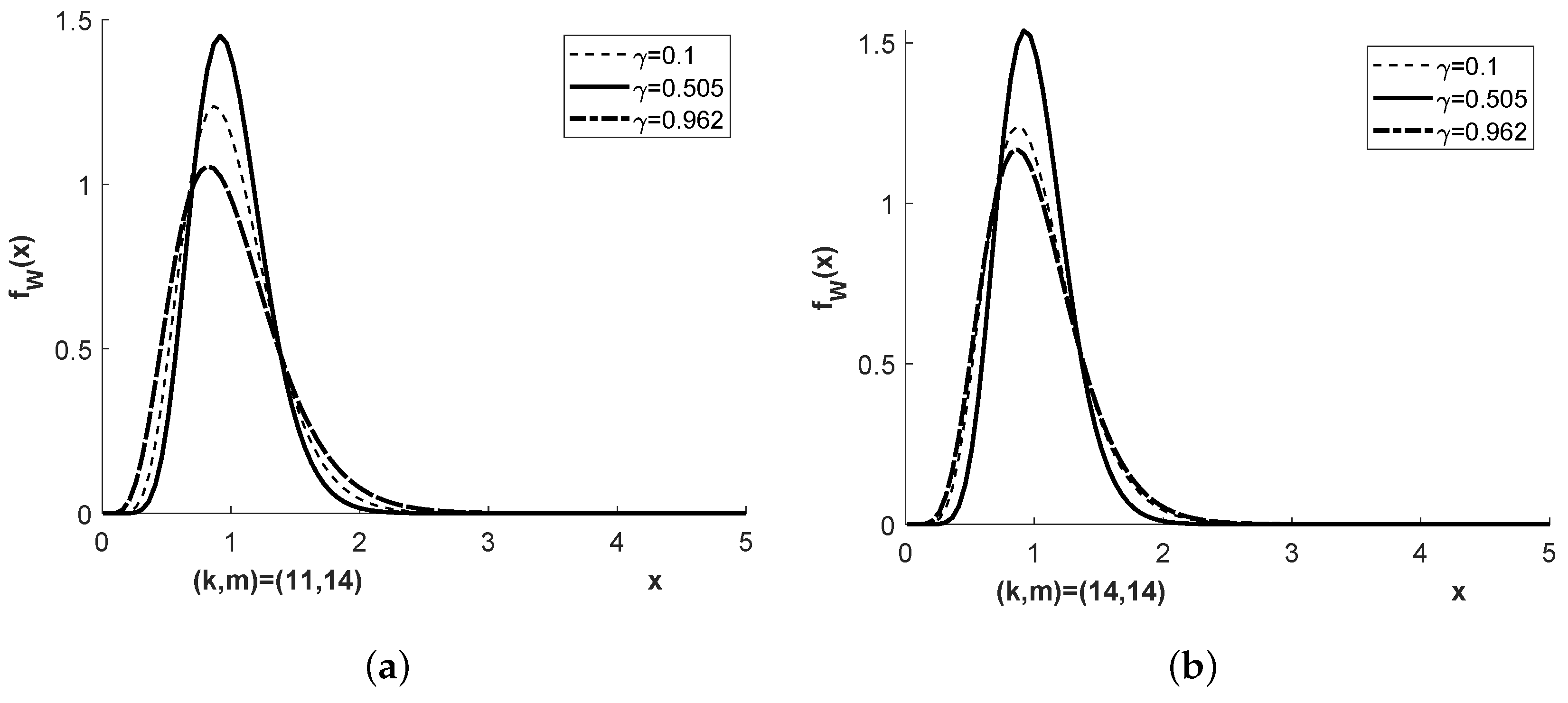
Definition 1.

The probability distribution having density (2) (or (3)) will be called chi-square bridge distribution with $(k,m)$ d.f. and mixing parameter γ, or $(k,m;\gamma )$-chi-square distribution ${\chi }_{k,m;\gamma }^2$, for short.

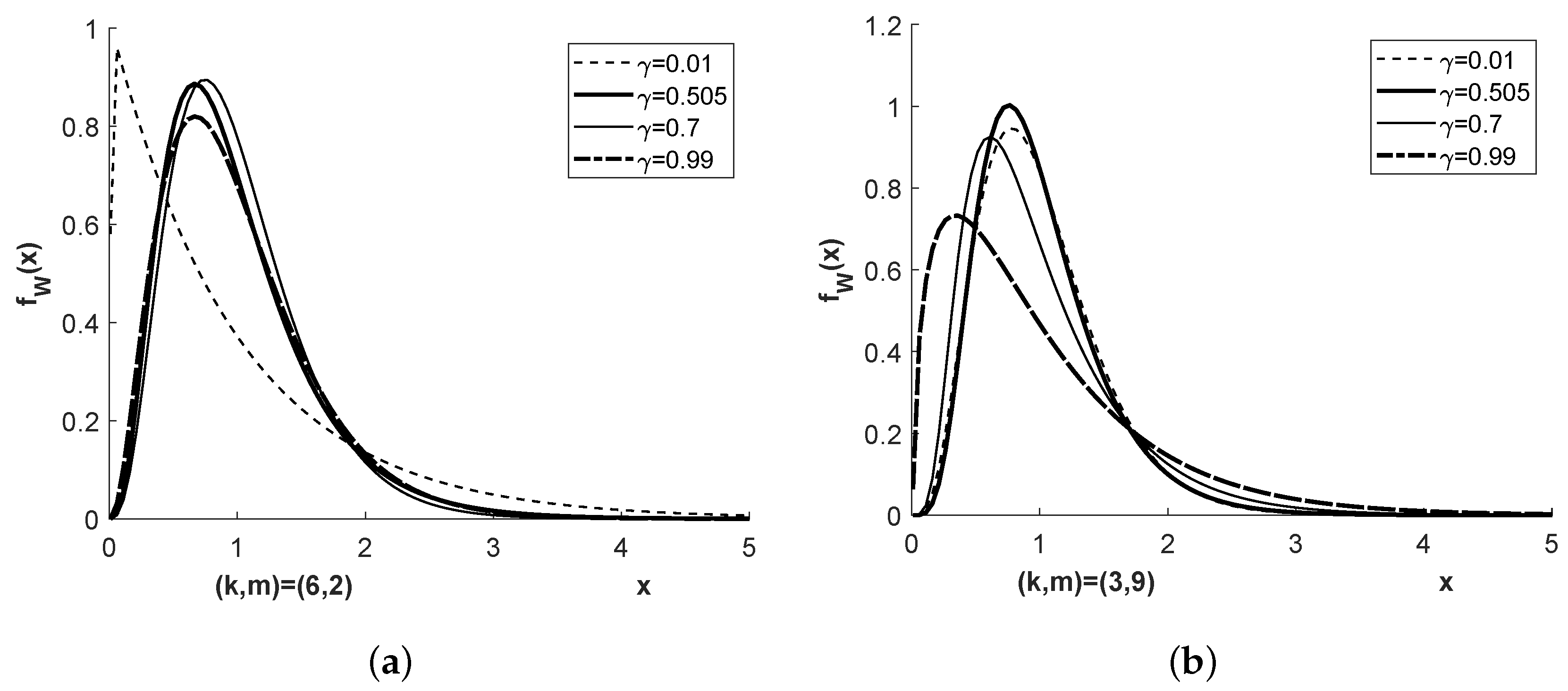
Figure 1 and Figure 2 show the density $f_W$ of the distribution ${\chi }_{k,m;\gamma }^2$ for four different pairs $(k,m)$, and $\gamma \in \{0.1,0.505,0.962\}$ or $\gamma \in \{0.01,0.505,0.7,0.99\}$, respectively.

3. Student Bridge Distribution

If N denotes a standard Gaussian distributed random variable that is independent of $C{Q}_{1,k}$ and $C{Q}_{2,m}$, and $t_l$ Student’s t-distribution with l d.f., then the statistic

$$T=T_{k,m;\gamma }=\frac{N}{\sqrt{WSCS(k,m;\gamma )}}$$

satisfies

$$T_{k,m;1}\sim t_k,T_{k,m;{\gamma }_0}\sim t_{k+m}\mathrm{and}{T}_{k,m;0}\sim t_m.$$

(4)

By the general integral representation of the density of the ratio of two independent continuous random variables,

$$f_T\left(t\right)=\underset{-\infty }{\overset{\infty }{\int }}{f}_N\left(tx\right)f_{\sqrt{WSCS(k,m;\gamma )}}\left(t\right)\left|t\right|dt$$

where $f_N$ denotes the standard Gaussian density and $f_{\sqrt{W}}\left(t\right)=2t{f}_W(t^2)$ can easily be derived from (2) or (3). Making use of (2) and changing the order of integration gives us:

$$\begin{array}{c}{f}_T\left(t\right)=\frac{2{(\frac{k}{\alpha })}^{k/2}{(\frac{m}{1-\alpha })}^{m/2}}{\sqrt{2\pi }{2}^{(k+m)/2}\Gamma (k/2)\Gamma (m/2}\hfill \\ ·\underset{0}{\overset{1}{\int }}{v}^{m/2-1}{(1-v)}^{k/2-1}\underset{0}{\overset{\infty }{\int }}{t}^{k+m-1}exp\{-\frac{t^2{x}^2}{2}-\frac{k{t}^2}{2\alpha }-\frac{-t^{2}v(\frac{m}{1-\alpha }-\frac{k}{2})}{2}\}tdtdv,\hfill \end{array}$$

and changing the variables $s=\frac{t^2}{2}(x^2+\frac{k}{\alpha }+v(\frac{m}{1-\alpha }-\frac{k}{2}))$ leads to the first of the following two alternative representations of the density $f_T$,

$$f_T\left(x\right)={\left(\frac{m\gamma }{k(1-\gamma )}\right)}^{m/2}\frac{\Gamma (\frac{k+m+1}{2}){}_2{F}_1\left(\frac{k+m+1}{2},\frac{m}{2};\frac{k+m}{2};\frac{\frac{k}{\gamma }-\frac{m}{1-\gamma }}{\frac{k}{\gamma }+x^2}\right)}{\Gamma (\frac{k+m}{2})\sqrt{\pi \frac{k}{\gamma }}{(1+\frac{\gamma }{k}{x}^2)}^{(k+m+1)/2}},x\in \mathbb{R}$$

(5)

and

$$f_T\left(x\right)={\left(\frac{k(1-\gamma )}{m\gamma }\right)}^{k/2}\frac{\Gamma (\frac{k+m+1}{2}){}_2{F}_1\left(\frac{k+m+1}{2},\frac{k}{2};\frac{k+m}{2};\frac{\frac{m}{1-\gamma }-\frac{k}{\gamma }}{\frac{m}{1-\gamma }+x^2}\right)}{\Gamma (\frac{k+m}{2})\sqrt{\pi \frac{m}{(1-\gamma )}}{(1+\frac{1-\gamma }{m}{x}^2)}^{(k+m+1)/2}},x\in \mathbb{R}.$$

(6)

Making use of (3) instead of (2) proves (6). Here, ${}_2{F}_1$ denotes the hypergeometric function being defined for $\delta >\beta >0$ by

$${}_2{F}_1(\gamma ,\beta ;\delta ;y)=\frac{1}{B(\beta ,\delta -\beta )}\underset{0}{\overset{1}{\int }}{(1-z)}^{\delta -\beta -1}{z}^{\beta -1}{(1-yz)}^{-\gamma }dz,$$

see 15.3.1 in [17] and Formula 9.111 in [18]. Choosing $y<0$ avoids a zero of $1-yz$ within the range of integration and might motivate a favor of using Formulas (5) or (6) if $\frac{k}{\gamma }<\frac{m}{1-\gamma }$ or $\frac{k}{\gamma }>\frac{m}{1-\gamma },$ respectively. The following definition is motivated by the three pillar bridges property (4).

Definition 2.

The probability distribution corresponding to density (5) (or (6)) will be called a Student bridge distribution with $(k,m)$ d.f. and mixing coefficient γ, or $(k,m;\gamma )$-Student bridge distribution $t_{k,m;\gamma }$, for short.

Figure 3 and Figure 4 show the density $f_T$ of the distribution $t_{k,m;\gamma }$ for the same choice of parameters as for $f_W.$

We remark that for $l=1,2,\dots ,$ $\mathbb{E}{T}^{2l-1}=0$ and

$$\begin{array}{cc}\hfill \mathbb{E}{T}^{2l}=& \frac{(2l-1)!!{\left(\frac{k}{\gamma }\right)}^{k/2}{\left(\frac{m}{1-\gamma }\right)}^{m/2}}{2^{(k+m)/2}\Gamma ((k+m)/2)}\hfill \\ \hfill & ·\underset{0}{\overset{\infty }{\int }}{x}^{\frac{k+m}{2}-1-l}{e}^{-\frac{kx}{2\gamma }}{}_1{F}_1\left(\frac{m}{2},\frac{k+m}{2},\frac{x}{2}\left(\frac{k}{\gamma }-\frac{m}{1-\gamma }\right)\right)dx,\hfill \end{array}$$

that is

$$\begin{array}{cc}\hfill \mathbb{E}{T}^{2l}=& \frac{\Gamma (\frac{k+m}{2}-l)}{\Gamma (\frac{k+m}{2})}{\left(\frac{k}{2\gamma }\right)}^l{\left(\frac{\gamma m}{(1-\gamma )k}\right)}^{m/2}\hfill \\ \hfill & ·{}_2{F}_1\left(\frac{k+m}{2}-l,\frac{m}{2};\frac{k+m}{2};1-\frac{\gamma m}{(1-\gamma )k}\right).\hfill \end{array}$$

4. Behrens–Fisher Statistic

Let $X_1,\dots ,X_{n_1}$ and $Y_1,\dots ,Y_{n_2}$ be jointly independent Gaussian samples with expectations ${\mu }_i$ and variances ${\sigma }_i^2,i=1,2.$ We consider the statistic

$$T^{BF}=\frac{\overline{X}-\overline{Y}}{\sqrt{\frac{S_X^2}{n_1}+\frac{S_Y^2}{n_2}}}$$

where $\overline{X}=\frac{1}{n_1}{\sum }_{i=1}^{n_1}{X}_i,\overline{Y}=\frac{1}{n_2}{\sum }_{i=1}^{n_2}{Y}_i$ and

$$S_X^2=\frac{1}{n_1-1}\sum _{i=1}^{n_1}{(X_i-\overline{X})}^2,S_Y^2=\frac{1}{n_2-1}\sum _{i=1}^{n_2}{(Y_i-\overline{Y})}^2$$

are common sample means and unbiased sample variances, respectively. By $Z\stackrel{d}{=}U$ we mean that two random variables Z and U have the same probability distribution.

Lemma 1.

The Behrens–Fisher statistic allows the representation

$$T^{BF}\stackrel{d}{=}\frac{Z_{n_1+n_2-1}}{\sqrt{S^2}}$$

with

$$S^2=A^{\ast }\sum _{i=1}^{n_1-1}{Z}_i^2+B^{\ast }\sum _{i=n_1}^{n_1+n_2-2}{Z}_i^2$$

and where ${(Z_1,\dots ,Z_{n_1+n_2-1})}^T$ is a standard Gaussian distributed random vector taking values in ${\mathbb{R}}^{n_1+n_2-1}$,

$$A^{\ast }=\frac{1}{1+\frac{n_1}{n_2}{(\frac{{\sigma }_2}{{\sigma }_1})}^2}·\frac{1}{n_1-1},B^{\ast }=\frac{1}{1+{[\frac{n_1}{n_2}{(\frac{{\sigma }_2}{{\sigma }_1})}^2]}^{-1}}·\frac{1}{n_2-1}$$

and

$$Z_{n_1+n_2-1}\stackrel{d}{=}\frac{\overline{X}-\overline{Y}}{\sqrt{\frac{{\sigma }_1^2}{n_1}+\frac{{\sigma }_2^2}{n_2}}}and{S}^2\stackrel{d}{=}\frac{\frac{S_X^2}{n_1}+\frac{S_Y^2}{n_2}}{\frac{{\sigma }_1^2}{n_1}+\frac{{\sigma }_2^2}{n_2}}$$

are independent.

Proof. 

We put

$$1_k={(1,\dots ,1)}^T\in {\mathbb{R}}^k,0_k={(0,\dots ,0)}^T\in {\mathbb{R}}^k,1^{+0}={\left(1_{n_1}^T{0}_{n_2}^T\right)}^T\mathrm{and}{1}^{0+}={\left(0_{n_1}^T{1}_{n_2}^T\right)}^T.$$

Let us further denote the orthogonal projection onto the linear space $\mathfrak{L}=\mathfrak{L}(1^{+0},1^{0+})$ by ${\Pi }_{\mathfrak{L}}$ and let the matrix P be defined such that ${\Pi }_{\mathfrak{L}}x=Px,\forall x\in {\mathbb{R}}^n$; $n=n_1+n_2,$ then

$$P=\left(\begin{array}{cc}\frac{1}{n_1}\mathrm{I}{\mathrm{I}}_{n_1}& \\ & \frac{1}{n_2}\mathrm{I}{\mathrm{I}}_{n_2}\end{array}\right)$$

where $\mathrm{I}{\mathrm{I}}_k=1_k{1}_k^T$ is a $k\times k$-matrix. Here and below, missing off-diagonal matrix elements are zero. If ${\mathfrak{L}}^{\perp }$ is the subspace of ${\mathbb{R}}^n$ being orthogonally to $\mathfrak{L}$ then $I_n-P={\Pi }_{{\mathfrak{L}}^{\perp }}$. The statistic $T^{BF}$ can be written as:

$$T^{BF}=\frac{\left({\pi }_{\mathfrak{L}}\left(\begin{array}{c}X\\ Y\end{array}\right),\frac{1}{n_1}{1}^{+0}-\frac{1}{n_2}{1}^{0+}\right)}{\left|\right|\left(\begin{array}{c}X\\ Y\end{array}\right)-{\pi }_{\mathfrak{L}}\left(\begin{array}{c}X\\ Y\end{array}\right){\left|\right|}_{\left(n\right)}}$$

(7)

where the functional ${\left|\right|.\left|\right|}_{\left(n\right)}$ is defined for all $x={(x_1,\dots ,x_{n_1})}^T\in {\mathbb{R}}^{n_1}$ and $y={(y_1,\dots ,y_{n_2})}^T\in {\mathbb{R}}^{n_2}$ as:

$$\left|\right|\left(\begin{array}{c}x\\ y\end{array}\right){\left|\right|}_{\left(n\right)}={\left(\frac{1}{n_1(n_1-1)}\sum _1^{n_1}{x}_i^2+\frac{1}{n_2(n_2-1)}\sum _1^{n_2}{y}_i^2\right)}^{1/2}.$$

We note that $P\mu =\mu$ and $(I_n-P)\mu =0_n$, and put $\kappa ={\left({\mu }_1{1}_{n_1}^T{0}_{n_2}^T\right)}^T.$ The random vector

$$\zeta =\left(\begin{array}{c}P\left(\begin{array}{c}X\\ Y\end{array}\right)\\ (I_n-P)\left(\begin{array}{c}X\\ Y\end{array}\right)\end{array}\right)$$

takes its values in ${\mathbb{R}}^{2n}$ and follows a singular Gaussian distribution of rank n,

$$\zeta \sim {\mathsf{\Phi }}_{\kappa ,\mathsf{\Psi }}\mathrm{with}\mathsf{\Psi }=\left(\begin{array}{cccc}\frac{{\sigma }_1^2}{n_1}\mathrm{I}{\mathrm{I}}_{n_1}& & & \\ & \frac{{\sigma }_2^2}{n_2}\mathrm{I}{\mathrm{I}}_{n_2}& & \\ & & {\sigma }_1^2(I_{n_1}-\frac{1}{n_1}\mathrm{I}{\mathrm{I}}_{n_1})& \\ & & & {\sigma }_1^2(I_{n_2}-\frac{1}{n_2}\mathrm{I}{\mathrm{I}}_{n_2})\end{array}\right).$$

As a consequence, the nominator and denominator of the ratio statistic $T^{BF}$ are stochastically independent. Let

$$B_1^T=\left(\begin{array}{cccc}{b}_1& \cdots & b_{n_1-1}& \frac{1}{\sqrt{n_1}}{1}_{n_1}\end{array}\right),B_2^T=\left(\begin{array}{cccc}{c}_1& \cdots & c_{n_2-1}& \frac{1}{\sqrt{n_2}}{1}_{n_2}\end{array}\right)$$

be orthogonal $n_1\times n_1$ and $n_2\times n_2$ matrices, respectively. The random vector $\eta =B(I_n-P)\left(\begin{array}{c}X\\ Y\end{array}\right)$ with $B=\left(\begin{array}{cc}{B}_1& \\ & B_2\end{array}\right)$ follows a centered Gaussian distribution with the covariance matrix

$$B\left(\begin{array}{cc}{\sigma }_1^2(I_{n_1}-\frac{1}{n_1}\mathrm{I}{\mathrm{I}}_{n_1})& \\ & {\sigma }_1^2(I_{n_2}-\frac{1}{n_2}\mathrm{I}{\mathrm{I}}_{n_2})\end{array}\right)B^T=\left(\begin{array}{cc}{\sigma }_1^2\left(\begin{array}{cc}{I}_{n_1-1}& 0\\ 0& 0\end{array}\right)& \\ & {\sigma }_2^2\left(\begin{array}{cc}{I}_{n_2-1}& 0\\ 0& 0\end{array}\right)\end{array}\right).$$

The vector $(I_n-P)\left(\begin{array}{c}X\\ Y\end{array}\right)=B^T\eta$ allows almost surely the representation

$$\begin{array}{cc}\hfill B^T\eta & =B^T{(N_1,\dots ,N_{n_1-1},0,N_{n_1+1},\dots ,N_{n-1},0)}^T\hfill \\ \hfill & =\sum _{i=1}^{n_1-1}{N}_i\left(\begin{array}{c}{b}_i\\ 0_{n_2}\end{array}\right)+\sum _{j=1}^{n_2-1}{N}_{n_1+j}\left(\begin{array}{c}{0}_{n_1}\\ c_j\end{array}\right)\hfill \\ & =\left(\begin{array}{c}{\displaystyle \underset{i=1}{\overset{n_1-1}{\Sigma }}}{N}_i{b}_i\\ {\displaystyle \underset{j=1}{\overset{n_2-1}{\Sigma }}}{N}_{n_1+j}{c}_j\end{array}\right)\hfill \end{array}$$

where the random variables $N_i$ are independent and centered normally distributed with variances ${\sigma }_1^2$ and ${\sigma }_2^2$ for $i=1,\dots ,n_1-1$ and $i=n_1+1,\dots ,n-1$, respectively. Let

$${B_1^{\ast }}^T=\left(\begin{array}{ccc}{b}_1& \dots & b_{n_1-1}\end{array}\right)\mathrm{and}{B_2^{\ast }}^T=\left(\begin{array}{ccc}{c}_1& \dots & c_{n_2-1}\end{array}\right).$$

The Kronecker product matrix ${B^{\ast }}^T={B_1^{\ast }}^T\otimes {B_2^{\ast }}^T=\left(\begin{array}{cc}{B_1^{\ast }}^T& \\ & {B_2^{\ast }}^T\end{array}\right)$ describes then a mapping from ${\mathbb{R}}^{2n-2}$ to ${\mathbb{R}}^{2n}$ and, a.s.,

$$\begin{array}{cc}\hfill \left|\right|B^T\eta {\left|\right|}_{\left(n\right)}& =\left|\right|\left(\begin{array}{c}{B_1^{\ast }}^T\left(\begin{array}{c}{N}_1\\ ⋮\\ N_{n_1-1}\end{array}\right)\\ {B_2^{\ast }}^T\left(\begin{array}{c}{N}_{n_1+1}\\ ⋮\\ N_{n-1}\end{array}\right)\end{array}\right){\left|\right|}_{\left(n\right)}^{\ast }\hfill \\ & =(\frac{1}{n_1(n_1-1)}\left|\right|{B_1^{\ast }}^T\left(\begin{array}{c}{N}_1\\ ⋮\\ N_{n_1-1}\end{array}\right){\left|\right|}^2+\frac{1}{n_2(n_2-1)}\left|\right|{B_2^{\ast }}^T\left(\begin{array}{c}{N}_{n_1+j}\\ ⋮\\ N_{n-1}\end{array}\right){\left|\right|}^2{)}^{1/2}\hfill \\ \hfill & =(\frac{1}{n_1(n_1-1)}\left|\right|\sum _{i=1}^{n_1-1}{N}_i{b}_i{\left|\right|}^2+\frac{1}{n_2(n_2-1)}\left|\right|\sum _{j=1}^{n_2-1}{N}_{n_1+j}{c}_j{\left|\right|}^2{)}^{1/2}\hfill \\ \hfill & =(\frac{1}{n_1(n_1-1)}\sum _{i=1}^{n_1-1}{N}_i^2+\frac{1}{n_2(n_2-1)}\sum _{j=1}^{n_2-1}{N}_{n_1+j}^2{)}^{1/2}\hfill \end{array}$$

where the norm ${\left|\right|.\left|\right|}_{\left(n\right)}^{\ast }$ is defined in ${\mathbb{R}}^{n-1}\times {\mathbb{R}}^{n-1}$. The variance of the nominator of the Behrens–Fisher statistic is

$$\mathbb{V}(\overline{X}-\overline{Y})=\frac{{\sigma }_1^2}{n_1}+\frac{{\sigma }_2^2}{n_2}.$$

Hence, $T^{BF}$ may be represented as

$$T^{BF}\stackrel{d}{=}\frac{(\frac{{\sigma }_1^2}{n_1}+\frac{{\sigma }_2^2}{n_2}{)}^{1/2}{N}_n}{(\frac{{\sigma }_1^2}{n_1(n_1-1)}{\displaystyle \underset{i=1}{\overset{n_1-1}{\Sigma }}}{N}_i^2+\frac{{\sigma }_2^2}{n_2(n_2-1)}{\displaystyle \underset{j=1}{\overset{n_2-1}{\Sigma }}}{N}_{n_1+j}^2{)}^{1/2}}$$

where the standard Gaussian distributed random variable $N_n$ is independent of $N_1,\dots ,N_{n_1-1},N_{n_1+1},\dots ,N_{n-1}$. □

The constants $A^{\ast }$ and $B^{\ast }$ from Lemma 1 depend on ${\sigma }_1$ and ${\sigma }_2$ only through the variance ratio $VR={\sigma }_2^2/{\sigma }_1^2$, which itself plays the role of a nuisance parameter.

If $\theta =VR/SR$ where $SR=\frac{n_2}{n_1}$ is the sample size ratio then the constants $A^{\ast },B^{\ast },VR$ and $n_2$ may be expressed in terms of the parameter triple $(\theta ,n_1,SR)$. The constants $A^{\ast }$ and $B^{\ast }$ depend on the variance ratio $VR$, but in a different way for the different sample size ratio $SR$. For $n_1$ given, the inverse mapping $(A^{\ast },B^{\ast })\to (\theta ,SR)$ is defined by:

$$\theta =\frac{1}{A^{\ast }(n_1-1)}-1,SR=\frac{1+A^{\ast }+B^{\ast }-A^{\ast }{n}_1}{n_1{B}^{\ast }}.$$

Other parameter triples could be introduced, e.g., $(k,m,\theta )$, being closely related to but nevertheless different from the parameter triple in [6].

The first and second order moments of $S^2$ are

$$\mathbb{E}{S}^2=1\mathrm{and}V\left(S^2\right)=\frac{2}{{(1+\theta )}^2}\left[\frac{1}{k}+\frac{{\theta }^2}{m}\right].$$

Finally, it turns out that under the hypothesis

$$H_0:{\mu }_1={\mu }_2$$

the statistic $T^{BF}$ allows the representation

$$T^{BF}{|}_{H_0}\stackrel{d}{=}\frac{N}{\sqrt{\gamma \frac{C{Q}_{1,n_1-1}}{n_1-1}+(1-\gamma )\frac{C{Q}_{2,n_2-1}}{n_2-1}}}$$

(8)

where the independent random variables N and $C{Q}_{i,n_i-i},i=1,2$ are as in Section 2, $k=n_1-1,m=n_2-1$, and the mixing coefficient is

$$\gamma =(1+\frac{VR}{SR}{)}^{-1}.$$

(9)

Thus, the Behrens–Fisher statistic follows the Student bridge distribution with d.f. $(n_1-1,n_2-1)$ and mixing coefficient $\gamma$, or $(n_1-1,n_2-1;\gamma )$-Student bridge distribution, for short,

$$T^{BF}{|}_{H_0}\sim t_{n_1-1,n_2-1;(1+\frac{VR}{SR}{)}^{-1}}.$$

(10)

In case of a known variance ratio, standard statistical significance testing and confidence estimation methods are based therefore upon the $(n_1-1,n_2-1;\gamma )$-Student bridge distribution in the common way. Here, assumption $\frac{k}{\gamma }<\frac{m}{1-\gamma }$ from Section 2 means that

$$\frac{n_1(n_1-1)}{n_2(n_2-1)}<\frac{{\sigma }_1^2}{{\sigma }_2^2}.$$

Without going here into technical details, the unrestricted distribution of $T^{BF}$ is a non-central Student bridge distribution in a suitably defined sense.

5. Discussion

5.1. Reflection of the Three Pillar Bridges Property

We now consider four examples from [8] for demonstrating the role the three pillar bridges property discussed in this paper may play in practical statistical work. In each example, we chose a pair of sample sizes $(k,m)$ from the set $\left\{\right(11,14),(14,14),(6,2),(3,9\left)\right\}$, and a variance ratio $VR$ from the positive real line that we assume to be known. In any case, we then determine the mixture coefficient $\gamma$ by a one-to-one calculation from $VR$. This way, Examples 1–4 are described (with some redundancy) as: $E1(11,14|1.25\left|0.505\right)$, $E2(14,14|0.04\left|0.962\right)$, $E3(6,2|1.25\left|0.505\right)$ and $E4(3,9|0.04\left|0.962\right)$. 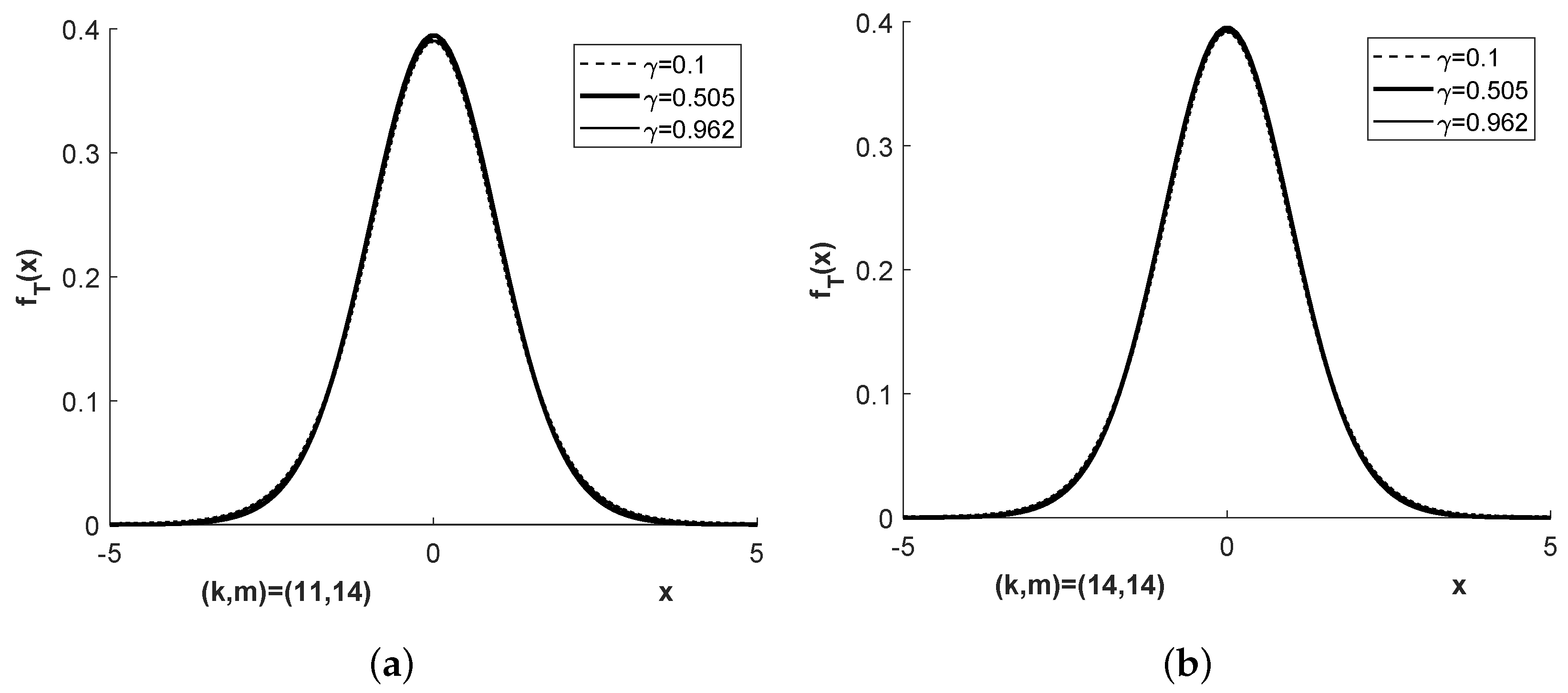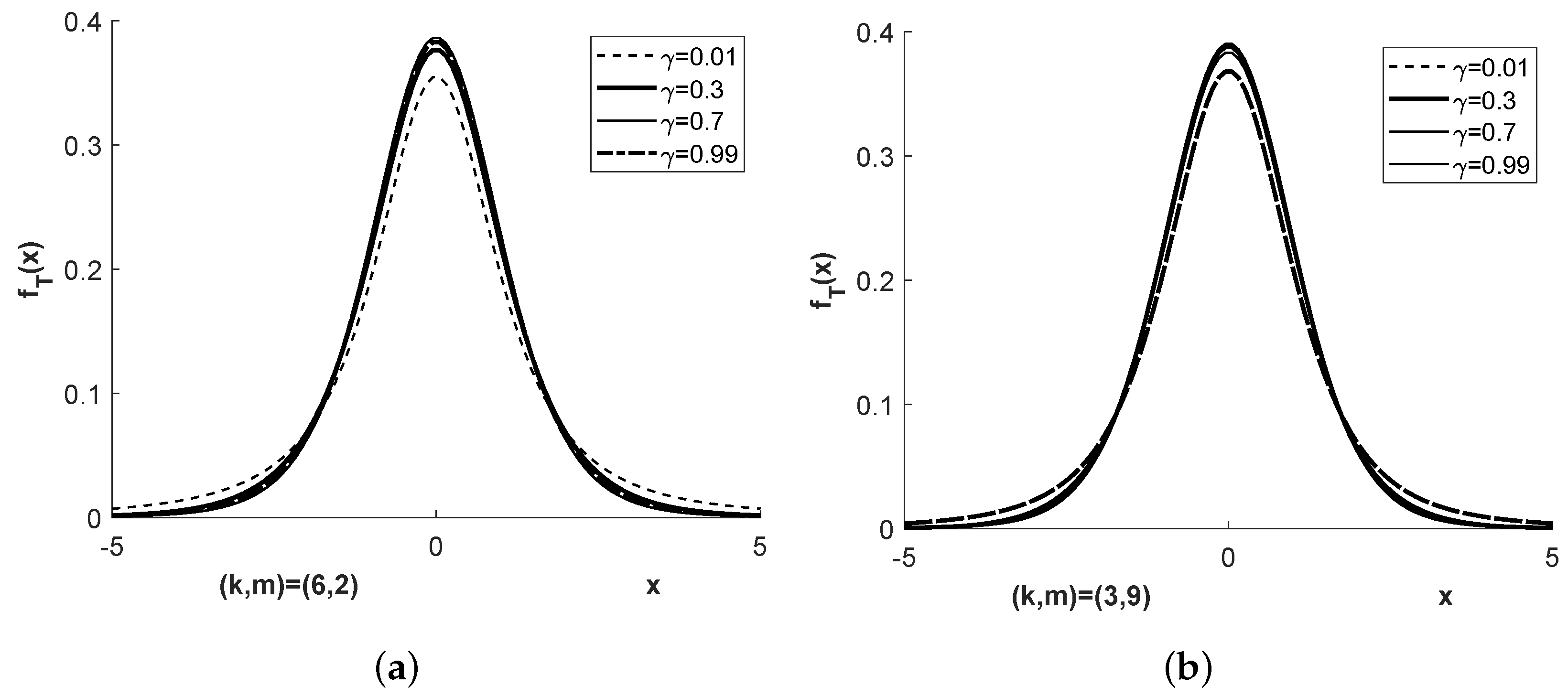Figure 1, Figure 2, Figure 3 and Figure 4 show the densities $f_W=f_{WSCS(k,m;\gamma )}$ and $f_T=f_{T_{k,m;\gamma }}$ for more parameter combinations $(k,m;\gamma )$ than required in Examples E1 to E4.

A value of $\gamma$ close to 1 corresponds to a value of $\theta =VR/SR$ close to zero, $VR<<SR$, meaning that the sample size in the second population compared to that in the first is disproportionately large compared to the corresponding quotient of variances; in other words, the first population is under represented.

A value of $\gamma$ close to 0 corresponds to a very large value of $\theta =VR/SR$, $SR<<VR$, meaning that the sample size in the first population compared to that in the second is disproportionately large compared to the corresponding quotient of variances; in other words, the second population is under represented.

Unlike these two cases of imbalance, a value of $\gamma$ in the order of ${\gamma }_0$ speaks for an approximately achieved balance. The latter can be observed close to the middle pillar of the three pillar Student bridge distribution and is suitable to explain some effect when choosing the degree of freedom in the Welch approximation to the exact density of T.

The chi-square bridge densities shown in Figure 1 correspond tho those of the Student bridge densities in Figure 3. It is shown in [8] that for such cases the Welch approximation seems to be the best that were found so far. Welch’s approximate degrees of freedom, see Formula (1.2) in [8] with $N_1-1=k,N_2-1=m$ and ${\sigma }_i^2$ replaced with $S_i^2,i=1,2$, are $f=25$ for Example 1 and $f=15$ for Example 2. This corresponds very well to the three pillar property of the Student bridge distribution.

If $\gamma =1/2$, as is approximately the case in Example 1, then the denominator $\mathcal{N}$ of T can be written as ${\mathcal{N}}^2=(C{Q}_{1,11}/11+C{Q}_{2,14}/14)/2.$ Because the numbers 11 and 14 are of comparable size, a reasonable approximation is ${\mathcal{N}}^2\approx (C{Q}_{1,11}+C{Q}_{2,14})/(2\times 12.5)\sim C{Q}_{25}/25$ finally leading for Example 1 to $T\approx t_{25}$.

In Example 2, the denominator of T allows the representation ${\mathcal{N}}^2=0.962C{Q}_{1,14}/14+0.038C{Q}_{2,14}/14$, which is reasonably approximated by ${\mathcal{N}}^2\approx C{Q}_{15}/15$. Thus, $T\approx t_{15}$.

Figure 2 shows a broader variability between the densities when the mixing coefficient $\gamma$ is varied compared to Figure 1. This is reflected in more visible variation of the corresponding Student bridge densities in Figure 4, both in their distribution centers and their distribution tails. This should be taken into account if applications of the Student bridge distribution are required, in particular in the areas of the distributions just mentioned.

The Welch approximation is known to perform better when both k and m are sufficiently large. Our Figures show what may happen for small sample sizes.

Because the consideration in [8] is even for higher dimensions it might be of some interest to extend the present work to this case, too.

5.2. Examples Where the Student Bridge Distribution Should Be Preferred

The aim of this section is to give a complementary structural argumentation confirming the numerical discoveries in [9] with respect to the question of when Welch’s approximation is not sufficiently precise. To this end, we present, for two cases of sample sizes and variance ratios, the exact Student bridge density and Welch’s approximation to it in a joint figure.

Example 5. Assume that as in Figure 1, Figure 2 and Figure 3 in [9], sample sizes $(n_1,n_2)$ are $(5,3),(3,4),(4,3),(2,4),(3,3)$ and $(2,2),$ and that the estimated variance ratio is always equal to 0.25. If we assume that the exact variance ratio in (10) is equal to 0.25, then the mixing coefficient $\gamma$ of the Student bridge distribution $t_{n_1-1,n_2-1;\gamma }$ is accordingly equal to 0.706, 0.840, 0.750, 0.889, 0.8 and 0.8. 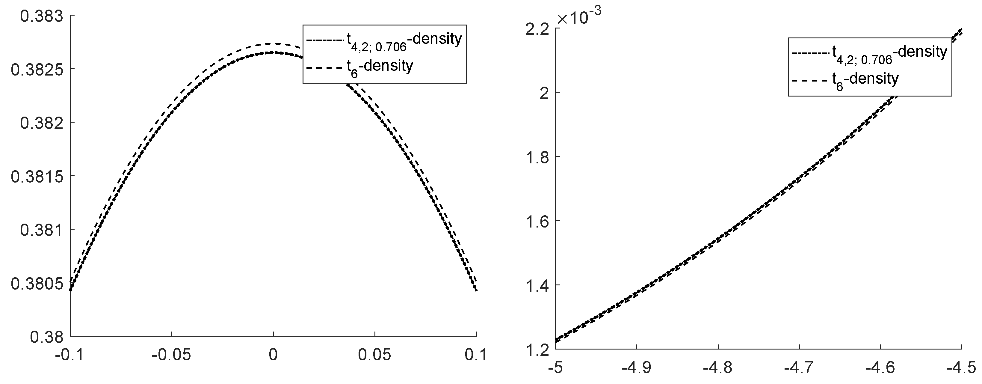Figure 5 shows the density of $t_{4,2;0.706}$ and the density of its Welch approximation $t_6$ that can hardly be visually distinguished from each other if considered on the whole line, but differ locally. 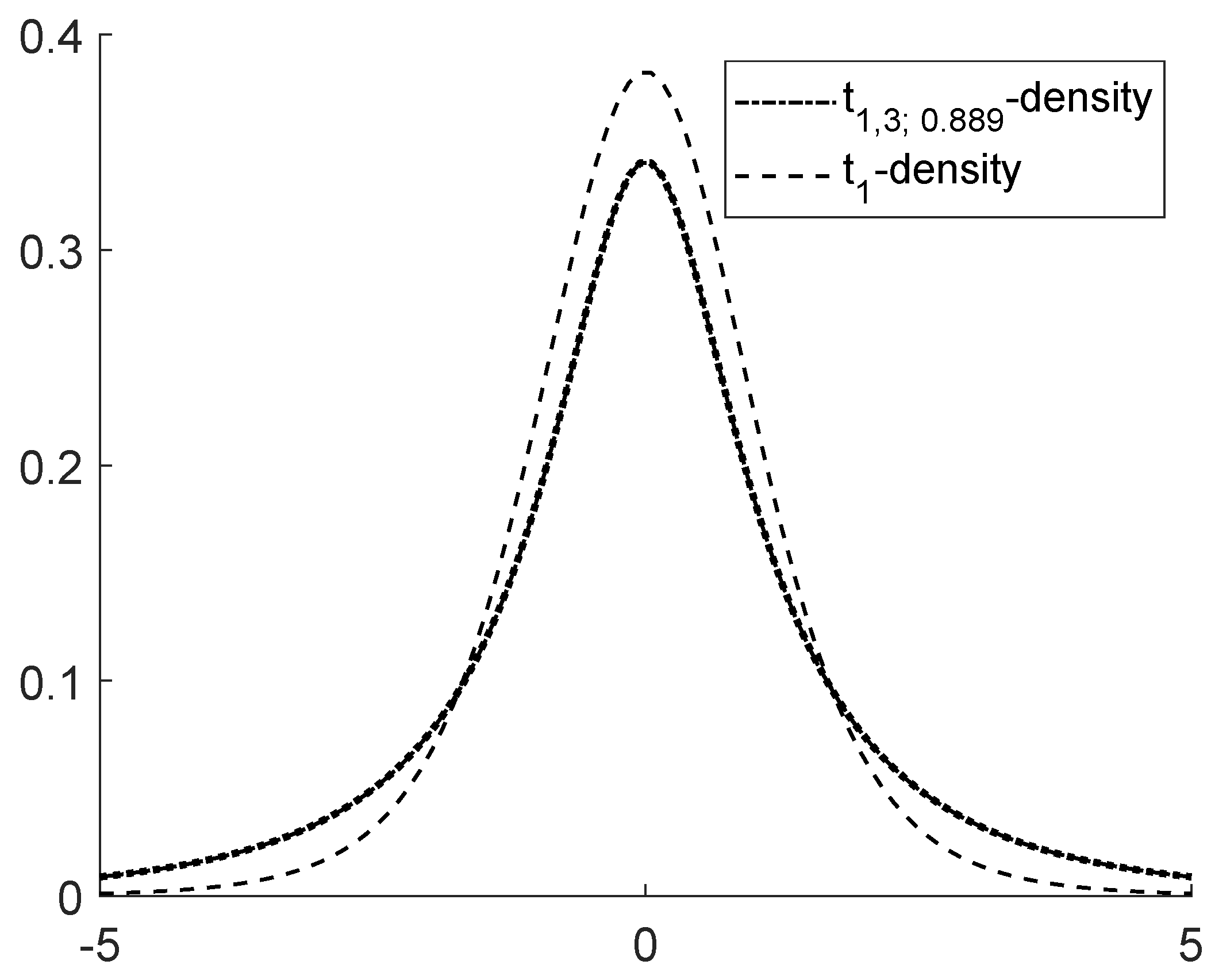Figure 6 shows the densities of the Student bridge distribution $t_{1,3;0.889}$ and Welch’s Student approximation to it, $t_1$. In this case, preference for the Student bridge density can even be seen globally.