Article

Application of the Modified Shepard’s Method (MSM): A Case Study with the Interpolation of Neogene Reservoir Variables in Northern Croatia

1
Faculty of Mining, Geology and Petroleum Engineering, University of Zagreb, HR-10000 Zagreb, Croatia
2
INA Plc., Zagreb, HR-10000 Zagreb, Croatia
3
Faculty of Science, University of Zagreb, HR-10000 Zagreb, Croatia
*
Author to whom correspondence should be addressed.
Stats 2020, 3(1), 68-83; https://doi.org/10.3390/stats3010007
Submission received: 8 December 2019 / Revised: 3 March 2020 / Accepted: 13 March 2020 / Published: 23 March 2020

Abstract

:
Interpolation is a procedure that depends on the spatial and/or statistical properties of the analysed variable(s). It is a particularly challenging task for small datasets, such as in those with less than 20 points of data. This problem is common in subsurface geological mapping, i.e., in cases where the data is taken solely from wells. Successful solutions of such mapping problems depend on interpolation methods designed primarily for small datasets and the datasets themselves. Here, we compare two methods, Inverse Distance Weighting and the Modified Shepard’s Method, and apply them to three variables (porosity, permeability, and thickness) measured in the Neogene sandstone hydrocarbon reservoirs (northern Croatia). The results show that cross-validation itself will not provide appropriate map selection, but, in combination with geometrical features, it can help experts eliminate the solutions with low-probable structures/shapes. The Golden Software licensed program Surfer 15 was used for the interpolations in this study.

1. Introduction

Geostatistics is a branch of applied statistics that applies theories of deterministic estimation and stochastic processes. These process are described as statistical inferences to different spatial phenomena in numerous branches of science. The most important geostatistical term applied in geology and petroleum geology is the regionalized variable [1], which indicates a measured or estimated magnitude whose behaviour is described in part by a random variable and in part by a deterministic variable. Such variables each show the properties of spatial continuity and, as such, are modelled in space. A qualitative description of the properties of a regionalized variable leads to a more accurate assessment of the regionalized variable.
The interpolation methods used in the Croatian part of the Pannonian Basin System (CPBS) are described in [2], while the final specific interpolation method that we applied is presented in [3]. The IDW method is widely used in the CPBS for mapping geological variables, and its application is described in [4,5,6,7,8].
The modified Sheppard’s method (MSM) has been applied all over the world. The following papers were selected as appropriate examples of this method. In [9], the authors applied the MSM to a digital terrain model region of the Chen-Yu-Lan River (Taiwan). The authors in [10] applied the MSM to multicomponent aerosol-cloud parameterization (global climate modelling), and the same method was used to model the calculations of hydrocarbon reserves [11]. The authors in [12] applied the MSM to selected parameters of subsurface waters in an area of approximately 10 ha located in the Ciemięga Valley (Poland). The MSM was used in [13] to determine the boundaries of the smooth particle hydrodynamics (SPH) method. The large number of measurements in this method enable the application of numerous algorithms with different mathematical complexities. However, Kriging, which uses different techniques, seems to be the most appropriate interpolation in most large datasets, such as in the creation of a digital terrain model [14]. However, even in such applications, methods like the modified Shepard’s method could be used, but their selection criteria, such as the homogeneity, variance, and density of their data, need to be clear [14]. Shepard’s method, although mathematically simple, could be improved. For example, in [13], the authors tested the numerical accuracy and calculation stability of smooth particle hydrodynamics. The authors proved that an improved Shepard’s method could have higher computational efficiency than the moving least square method, the simplified finite difference interpolation method, or the normalized interpolation method.
Furthermore, although Kriging is the best linear estimator, it is not always the best choice for model visualisation. For example, for a small dataset [15], the inverse distance weighting algorithm was used to interpolate data collected from 20 solar radiation monitoring stations in central and southern Taiwan.
The authors in [16] presented the creation of a coherent and continuous digital elevation model (DEM) of a riverbed using four interpolation methods. These methods are: inverse distance weighting (IDW); a radial basis function (RBF) with a completely regularized spline (CRS); Simple Kriging (KRG), which is a geo-statistical method; and Topo to Raster (TopoR), a particular method specifically designed for creating continuous surfaces from various elevation points, contours, or polygon data, suitable for creating surfaces for hydrologic analysis. The last method was evaluated to be the most accurate, and IDW and RBF were the methods with the largest errors.
Another study considered the generation of digital elevation models (DEMs) from global navigation satellite systems (GNSS) [17]. The authors interpolated DEMs, with resolutions ranging from 0.5 to 10 m, using the natural neighbour (NaN), Topo to Raster (ANUDEM), and inverse distance weighted (IDW) methods. The Topo to Raster method resulted in the largest DEM accuracy, while the IDW method resulted in the lowest. Interestingly, NaN produced “a more visually appealing surface”, i.e., more interpretable shapes.
Consequently, we decided to use the modified Shepard’s method compared with inverse distance weighting in a selected area, to determine alternative methods for the proper visualisation of small datasets of reservoir variables in northern Croatia. This method was applied to the hydrocarbon field “B” and the Late Miocene (Lower Pontian) reservoir “K” considering three geological variables: porosity, permeability, and thickness.

2. Geological Settings of the Analysed Field “B” (Sava Depression, Northern Croatia)

Oil and gas field “B” is located in the CPBS, i.e., in the western part of the Sava Depression. The location of field “B” in the depression is shown in Figure 1.
Most of the wells reach the base of the Kloštar Ivanić Formation, since hydrocarbon reservoirs occur within this formation, which is described as an alteration of marls and well-sorted sandstones. In the deepest part of the well, the sandstone is hard. This sandstone is replaced by fine-grained and weakly consolidated sand in the upper part. The marls are grey to greyish-brown, with medium hardness; their compaction decreases upwards, followed by an increase in the proportion of their clay components. The marls comprise the impermeable rocks on top of each sandstone reservoir. Within the studied formation, the marl’s thickness is 30–150 m, while the sandstone’s thickness is 20–150 m.
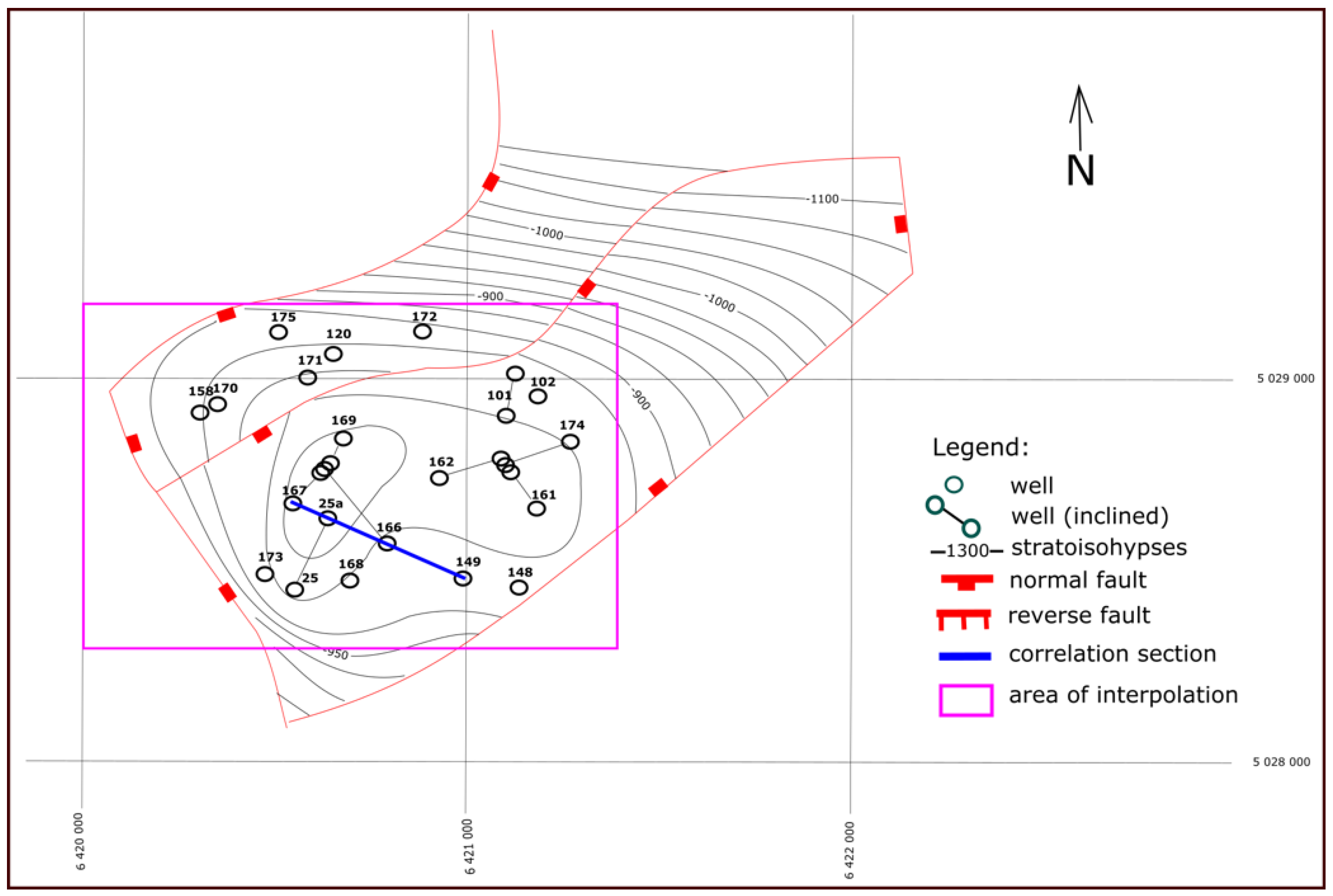
Structurally, in most cases, tectonic blocks are considered to represent separate structural traps, where hydrocarbons are accumulated in the highest parts. Therefore, these tectonic blocks represent separate hydrodynamic units with similar reservoir characteristics. A structural map of the analysed Late Miocene (Lower Pontian) reservoir “K” is shown in Figure 2.
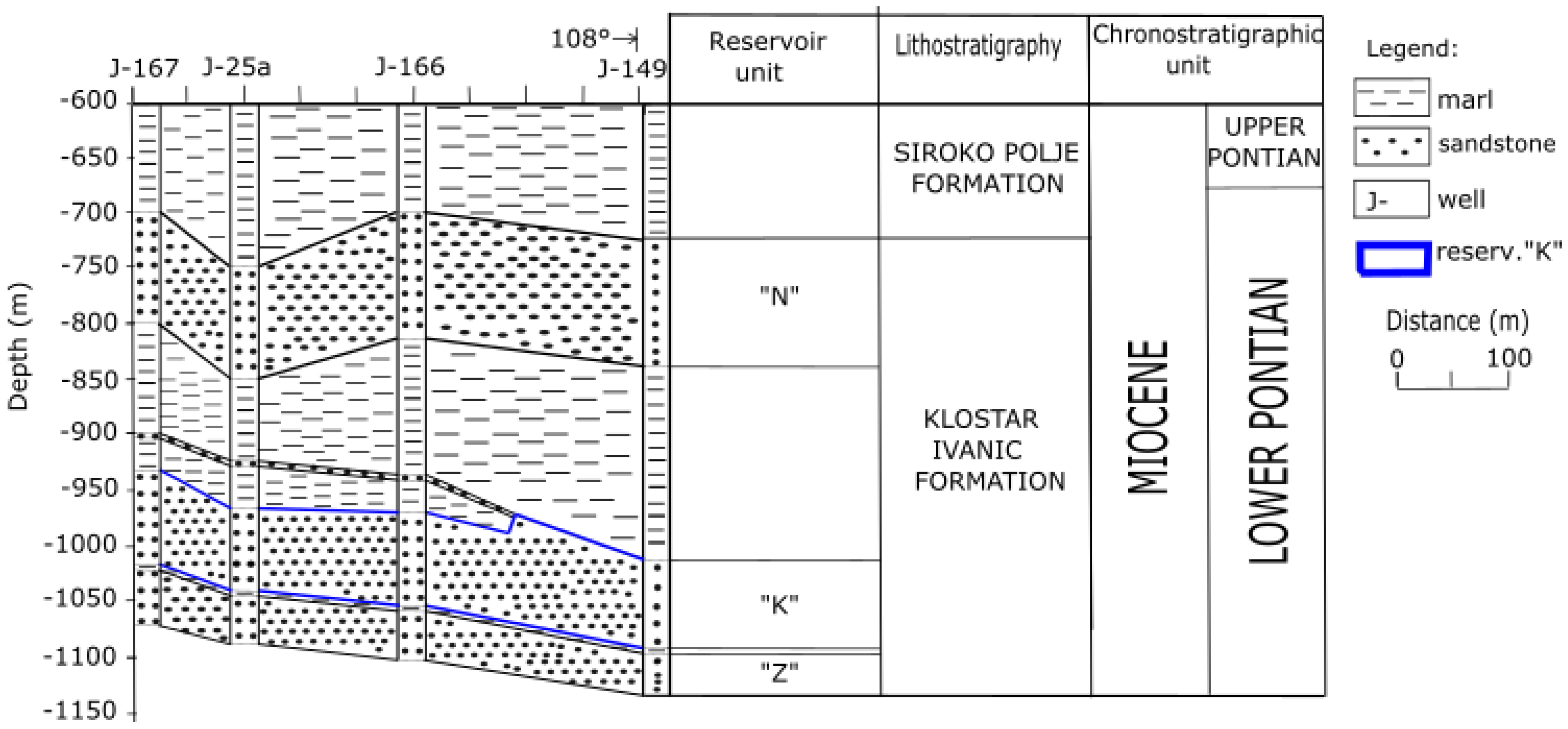
A typical geological section is derived from the well data, and clearly outlines the sandstone member (blue borders) with discovered hydrocarbon reservoirs (see Figure 3). The section also reveals a partial structural inversion within the formation, where monocline of deeper members is transformed into the syncline in the upper part.
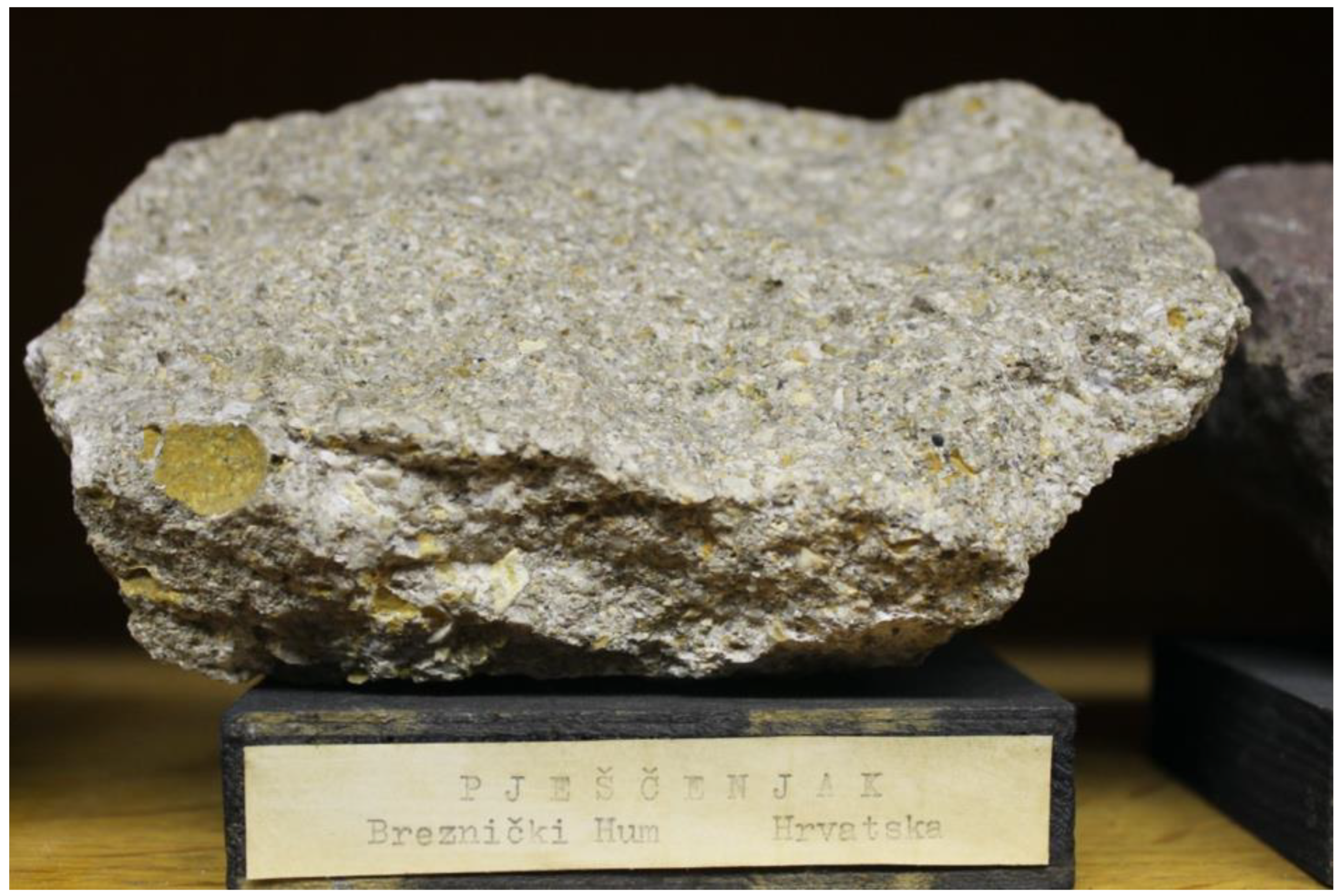
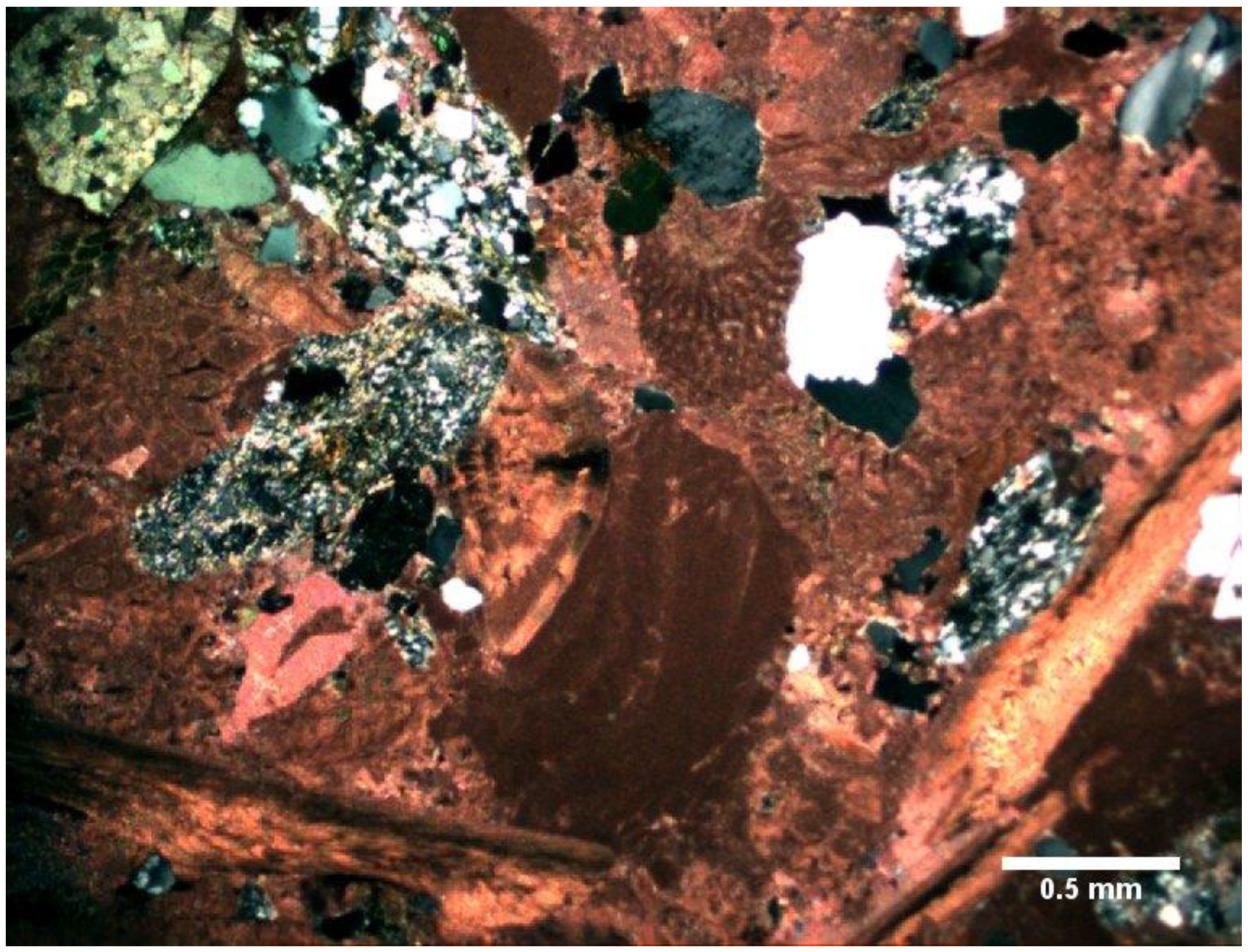
The mapped sandstone “K” could be described as one of two typical sandstone types in the northern Croatian Neogene. The younger sandstones, well-sorted, medium-grained, quartz-mica dominated, were deposited in the lacustric, mostly brackish environment of Pannonian Lake. The detritus was transported by sequential turbidites during the Late Miocene (Upper Pannonian and, especially, Lower Pontian) (e.g., [19]). The dominant, primary porosity is intra-granular. The second, older type comprises poorly sorted and coarse-grained sandstones, containing some larger (ruditic) clasts, which are bound together with sparry calcite cement. They contain various lithoclasts derived from older sedimentary and metamorphic rocks: dolomites, quartzites, gneisses and various schists, as well as individual quartz grains which originated from metamorphic rocks. Such calcareous sandstones (e.g., [20,21]) were deposited during the Middle Badenian, in the shallow marine back-reef environments of the Paratethys Sea, with a significant input of siliciclastic material from the nearby land (see Figure 4). The dominant, primary porosity is intra-skeletal (see Figure 5).
The object of this research, the “K” reservoir, currently produces hydrocarbons using a secondary method (water injection). This is a very maturely explored and developed area, which allows significant improvements and upgrades of geological models in order to increase hydrocarbon recovery. This is especially reflected in the application of statistical and geomathematical analyses of numerous reservoir variables such as porosity and permeability (primary variables) and injected water volumes (secondary variable). Furthermore, most of the existing reservoirs maps (structural, porosity, etc.) should be redrawn in much more detail, using ever-advancing mapping algorithms.
Mathematical algorithms, such as variograms and Kriging, have been the main tools in analysing spatial dependence and the possible anisotropy of the selected variables in the CPBS. However, for a small input dataset, like the injected volume of water (three points of data) and permeability (18 points of data), simpler interpolation methods such as: Inverse Distance, Nearest and Natural Neighbourhood are more effective, e.g., 15 points of data were sufficient to apply the Inverse Distance and Nearest Neighbourhood methods, and even for reservoir characterisation in cases of very low numbers of datasets (e.g., [22]). However, the problem of visually expressed local values (“bull’s-eye”, “butterflies”) permanently exists and can lead to misinterpretation. That is the reason for testing the modified Sheppard’s methods in this study, as a replacement for using the IDW method, leading to similar cross-validation results and, visually, a lower number of non-acceptable geological shapes.
The interpolation of porosity, permeability and thickness of the Neogene sandstone reservoir “K” in northern Croatia, is valid for all similar reservoirs in the CPBS. This also means that the applied methods, interpretations and conclusions could be applied in the Middle Miocene (Badenian) as well as in the Upper Miocene (Pannonian/Pontian) sandstones in this area, even though their origin is partially different.

3. Basics of the Applied Interpolation Methods

Interpolation is an estimation of the values of variables in places where no values have been measured. When interpolating, one (primary) or multiple (primary + secondary) variables can be used. The interpolation methods applied in reservoir “K” are Inverse Distance Weighting (IDW) and the Modified Shepard’s Method (MSM). Only primary variables (porosity, permeability, thickness) were used.
This was a bi-dimensional interpolation, standardised for hydrocarbon reservoirs. “Standardisation” means that each point of data represents one well and an interval of a well drilled through a selected reservoir. The selected value is an average across the reservoir interval, and Figure 3 also schematically depicts average depths, lithology and structural position, e.g., in [23]. The average values are calculated from logs or cores, which were not a part of this study, i.e., such average values were taken from available reports. 2D reservoir interpolation is the conventional procedure for reservoirs of low to medium thickness (in general, less than 50 m) and which are of mostly homogenous composition (the majority of sandstone reservoirs are often approximated as homogeneous, much like the one being analysed). Examples of different reservoir interpolations in northern Croatia have been vastly made in 2D space and have been published in numerous papers. Here, selections were made in geological depositional environments similar to the Sava Depression (as in the situation here) and the Drava Depression (just to the north), which are the two largest depressions in the CPBS. The choice to apply 2D interpolation (vs. the 3D possibility) had been made without regard to method selection (hand-made, software with statistical or geostatistical algorithms. All case reservoirs of lithostratigraphic units had been considered as vertically uniform sections, regardless of the selected variable. Such regional and local structural interpolation can be clearly observed on the map published for the Bjelovar Subdepression (hand-made interpolation given in [24]) or the Kloštar Structure in the Sava Depression [25]. In the same structure, even geostatistical sequential indicator simulation of porosity and thickness had been made with 2D interpolation [26]. Even back in the Bjelovar Subdepression, when the thickness had been remapped by Kriging, it was done in 2D space (e.g., [27,28]). Finally, 2D interpolation in the same region as selected in this analysis, had been especially favourable when the input dataset was small, regardless of whether the interpolation was done by statistical or geostatistical methods [3,19].
As previously mentioned, 3D interpolation is a useful approach when the mapped unit is heterogeneous, and can be precisely defined from the available data (like logs or cores). If such data are ambiguous, then it is much more appropriate to apply 2D interpolation and avoid any heterogeneity which cannot be accurately interpreted. Moreover, in a large number of cases, the mapped variable (thickness, porosity, permeability) does not depend on indirect variables such as topography or well length, because such variables are collected in a single unit with the same depositional history, which is a critical element. Even if the depths are mapped, the “problem” of topography is often easily solved using a datum plane (in the entire CPBS it is +100 m). All these facts outline why 2D mapping is a valid procedure for this analysis, and not 3D.

3.1. Inverse Distance Weighting (IDW)

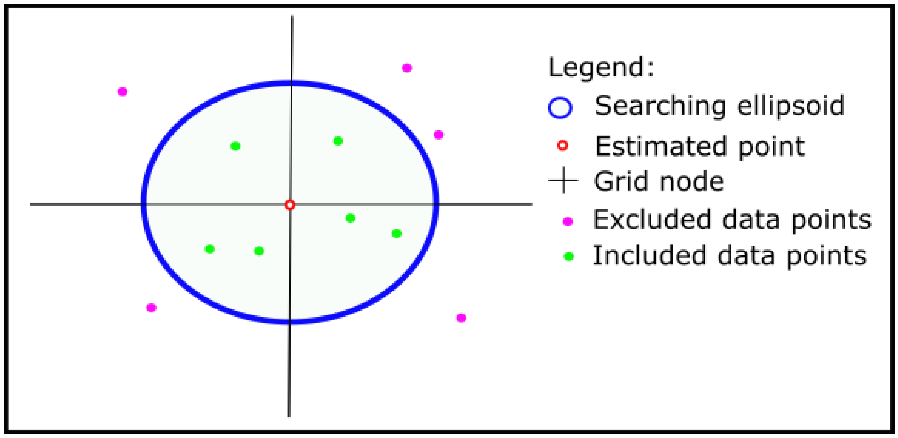
The Inverse Distance Weighting method is a mathematically simple interpolation method, where the unknown value of a variable is estimated according to the known values inside the searching radius (radii). The radii of such an ellipsoid (see Figure 6) or the radius of a circle can include some data points, but generally, most software includes all points that are geologically (or in some other way) connected by default.
In any case, a searching area could be a radius (a searching circle) or radii (a searching ellipsoid), which covers both options available in 2D interpolation. We did not discuss a 3D option, because it would produce a spheroid, which was not used here, and software mostly approximates a spheroid with two perpendicular ellipsoids (thus software does not construct a real spheroid, but only three perpendicular axes).
Generally, each point is weighted by distance (see Figure 6). A single datum is inversely proportional, dependent on the distance between the unknown and the measured values of a variable.
The estimation (e.g., [29,30]) in IDW is done using Equation (1):
z I U = z 1 d 1 p + z 2 d 2 p + z n d n p 1 d 1 p + 1 d 2 p + 1 d n p
where:
ziu—interpolated (unknown) value;
di—distance to “i-th” location;
zi—interpolating (known) value at “i-th” location;
p—power of distance.

3.2. Modified Shepard’s Method (MSM)

MSM interpolation is a modification of the IDW method, with the aim of reducing the expressive local values (outliers, extremes) that could cause “bull-eyeing” or “butterfly shape” effects. The method was developed by [31], sometimes named as Shepard’s method, and modification of the method was carried out in the works of, for example, [32,33,34]. An estimation (e.g., [33,34]) using the MSM function is shown by Equation (2):
F ( x , y ) = k = 1 n W k ( x , y ) · Q k ( x , y ) i = 1 n W i ( x , y )
where:
F—MSM function;
W—relative weights;
Qk—bivariate quadratic function;
x, y—data coordinates;
n—number of data.
A bivariate quadratic function is a second-degree polynomial of the form f ( x , y ) = a x 2 + b y 2 + c x y + d x + e y + f where x and y are variables, a,b,c,d,e variables, f is constant. Such a function describes a quadratic surface. Setting f(x,y) = 0 describes the intersection of the surface with the plane z = 0, which is a locus of points equivalent to a conic section.
The MSM uses so-called relative weights determined (e.g., [33]) with Equation (3):
W k ( x , y ) = [ ( R ω d k ) + R ω · d k ] 2
where:
W—relative weights;
dk—Euclidean distance between points at locations (x, y) and (xk, yk);
Rω—radius of influence around node (xk, yk).
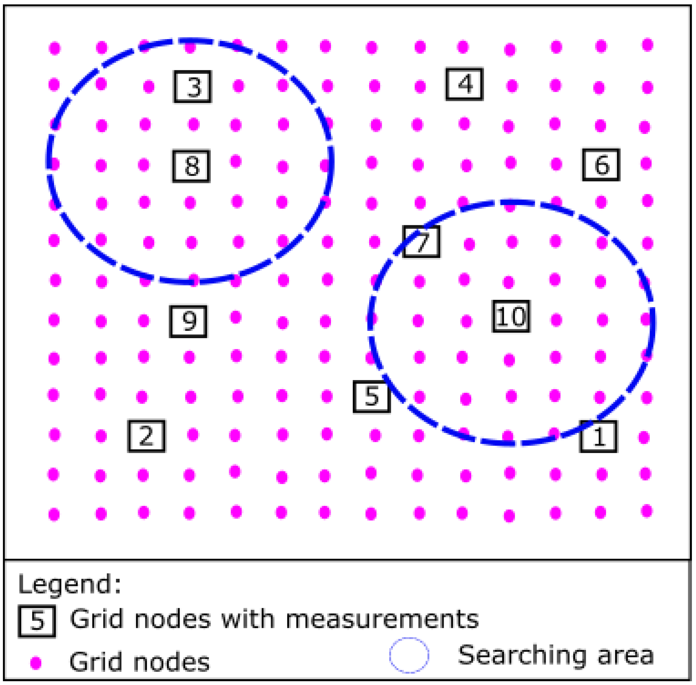
Figure 7 shows the searching radii of the MSM within the measured and estimated values (grid). Here it can be noted that each unknown point is surrounded with local searching radii, instead of global, like in the IDW method.

3.3. Cross-Validation (CV)

The algorithm or the cross-validation is rather simple (see Equation (4)), where some data (or a cluster of data) has been “deleted” and the estimation is performed from the remaining data. This procedure is often called “Mean Square Error” (MSE), due to the squaring data differences. Such a re-sampling method is characterized by dimensionless standard error. The famous pioneer work on cross-validation was published by [35] and one classical application of MSE in the CPBS has been published in [6].
In geological mapping, the MSE has been applied to get a value that shows a numerical error obtained from the same dataset interpolated by a different method (algorithm). In our case, if the porosity, permeability or thickness are mapped while simultaneously using IDW and the MSM, each map, although constructed from the same data, will have a different visual outcome (shape) and a different MSE value. In general, a lower MSE means better interpolation, but a numerical value cannot be the only criteria for quality evaluation. The calculation of MSE can be applied to all geological variables.
M S E = 1 n i = 1 n ( m e a s u r e d e s t i m a t e d ) 2
where:
MSE—value of cross-validation, i.e., mean square error;
measured—value measured d at location “I”;
estimated—value estimated at location “I”;
n—number of locations.
The cross-validation applied in this analysis has been included as one of the software (Golden/Surfer) features. According to the given definition, all points were deleted one-by-one, i.e., sequentially. This means that in the “n-th” iteration, only one point was deleted, as the equation condition allows (see Equation (4)).

4. Interpolation Results in Reservoir “K” for Variables of Porosity, Thickness and Permeability

Here are three interpolated geological variables, measured in reservoir “K”, namely: porosity, permeability and thickness. Table 1 and Table 2 shows the part of their descriptive statistics, calculated from values measured from the laboratory measurement and/or interpretation of the logging curves (resistivity, density and neutron).
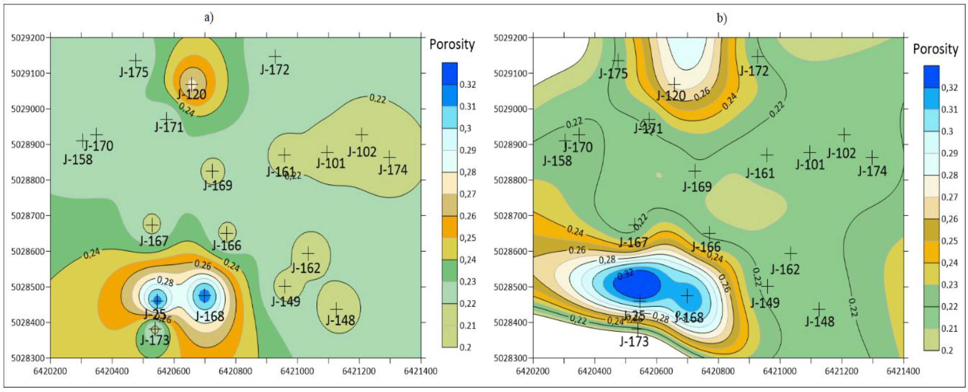
According to Table 1, the analysed sets belong to a small geological input data set [8,36]. So, interpolation has been done with mathematically simpler methods. The porosity maps obtained by the IDW and MSM methods are shown in Figure 8. The value cross-validation (porosity) for IDW is 0.00119 and MSM is 0.00345. The other crucial parameters for interpolation presented in Figure 8, Figure 9 and Figure 10 are: power exponent 2, grid size 50 × 50 cells, searching radii 1/2 of primary and secondary reservoir axes (the boxed/interpolated area in Figure 2).
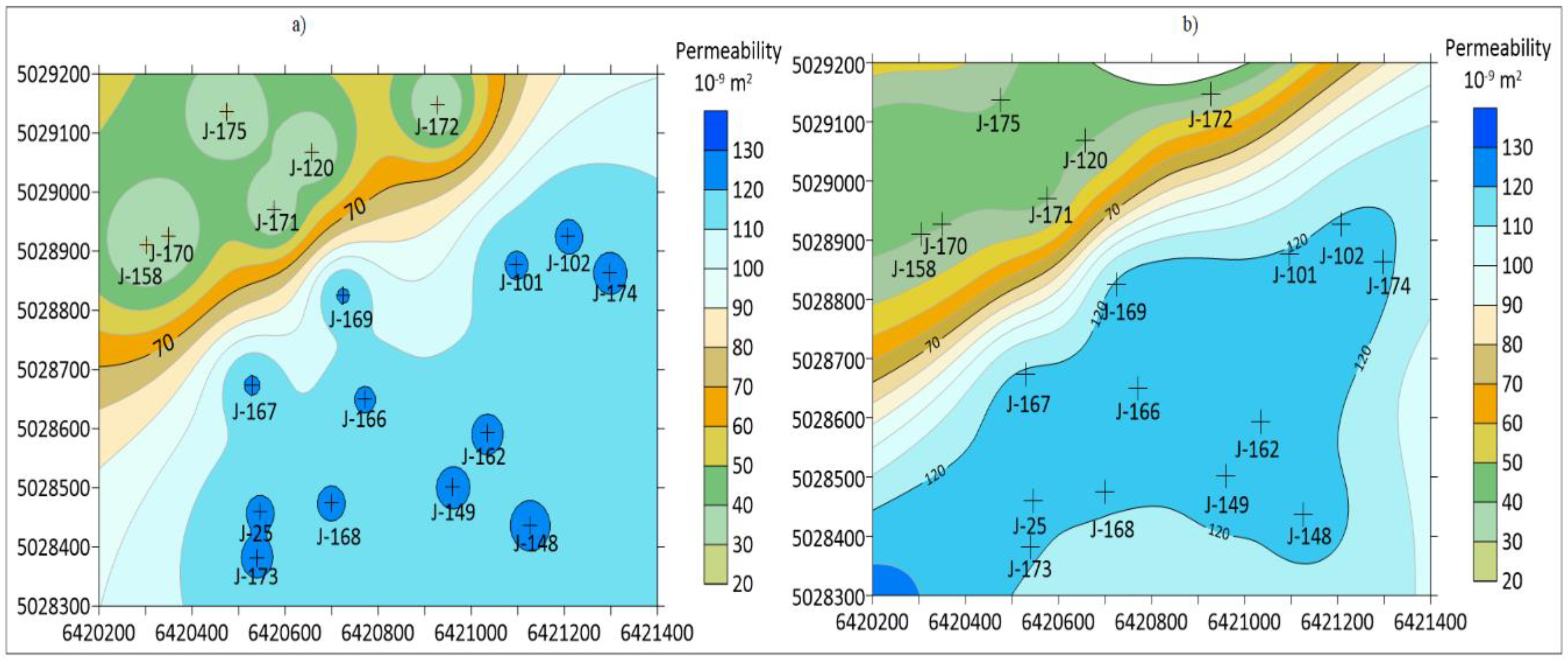
Permeability maps obtained by the IDW and MSM methods are shown in Figure 9. The accompanied cross-validation (permeability) for IDW is 480.8 and MSM 516.1.
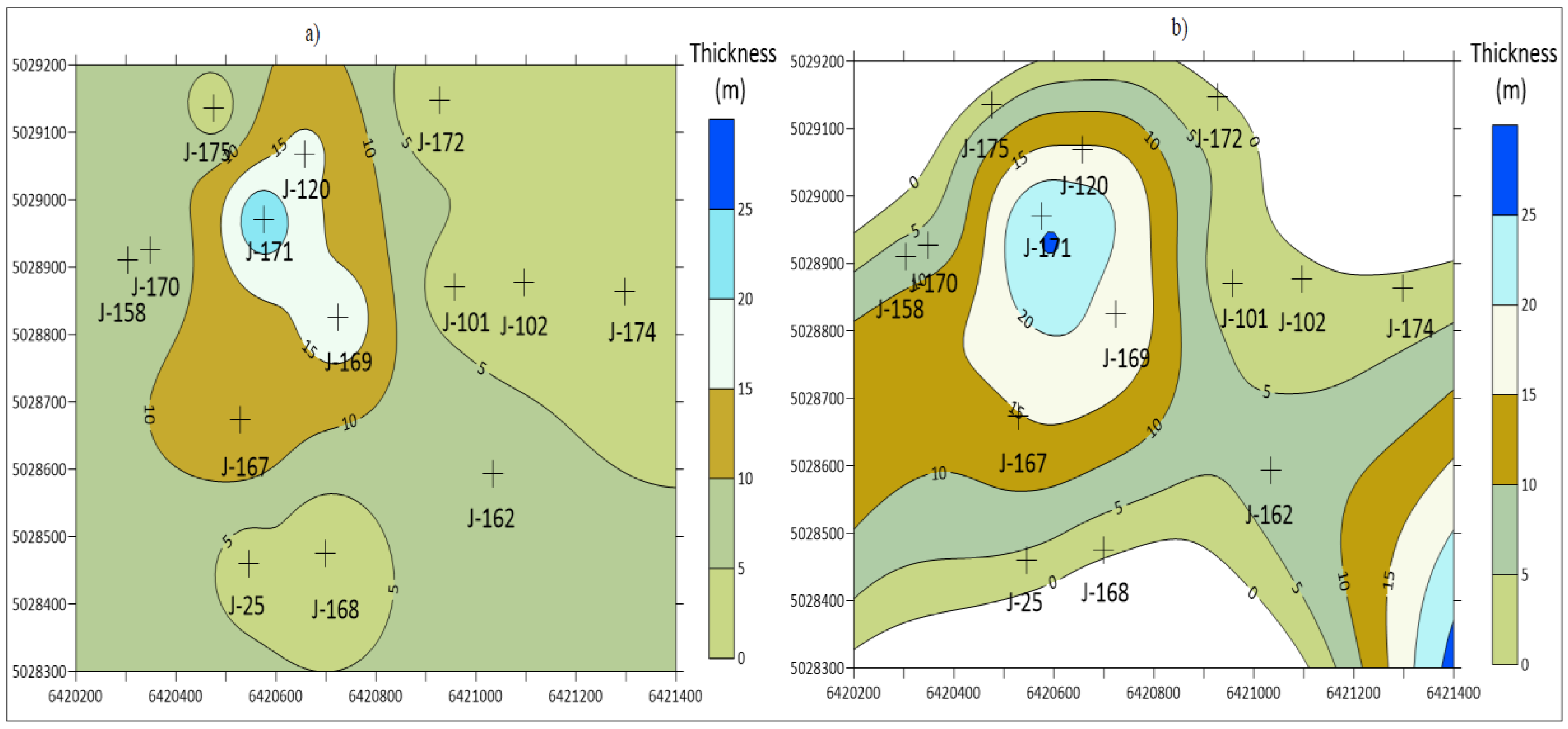
Thickness maps which have been interpolated by the IDW and MSM methods are shown in Figure 10. The value cross-validation (thickness) for IDW is 40.7 and MSM is 60.5.
The maps obtained through the IDW and MSM methods are evaluated in a quick-look, according to the most observable feature of a highly expressed local value, i.e., bull-eye or butterfly shape effects. The MSM is clearly advantageous because it mitigates the mentioned effects, however a numerical review using the cross-validation values strongly favours the IDW method.

5. Discussion

To consider the differences between the results obtained with the IDW and MSM methods, it is necessary to discuss the main differences in their equations. The IDW method does not use a weighting coefficient, i.e., each value is “weighted” by a simple (powered) inversely proportional distance from the measured point. The general form of the IDW method is Equation (5):
u ( x ) = i = 1 N w i ( x ) · u i i = 1 N w i ( x ) ,   d ( x , x i ) 0
where:
u(x)—interpolated value in the location “x”;
uii-th known value inside searching radius(es) centred in the location “x”;
i—no. of samples (known/measured value);
wi—weight for the “i-th” sample with known value;
N—number of samples with known value.
So, the weighting coefficients for the location “x” could generally be defined as Equation (6):
w i ( x ) = 1 d ( x , x i ) p
where:
wi—weight for location “x”;
d(x,xi)—is a given distance (metric operator) from the known point xi to the unknown point x,
p—power factor (positive real number).
This is a basic IDW function as defined by Shepard ([31], where weights decrease as distances to the known values increase. On the other hand, higher values of power (“p”) favour a larger influence of measured points closer to the interpolated point, and eventually ended up in a zonal interpolation (like a Voronoi diagram), where the inside zone is used as a constant value of a single known point centred into such a polygon and no isolines are constructed. On the contrary, for a 2D interpolation, if the power is 2 (like we used here and based on the previous interpolation done in the CPBS) or less, more distanced measured points will have a greater influence. In the “M” dimensions, this statement is valid for p ≤ M. In all cases, IDW minimizes the function that measures deviation between the unknown and known points using the condition Equation (7):
δ ( x , u ) δ u = 0
On the contrary, the MSM is a more advanced technique than IDW, including a weighting coefficient (see Equation (8)), and calculating the interpolated value using only the nearest known points within the R-sphere (instead of using a full set of measured samples, which is the default setting of IDW in numerous algorithms). Weights are modified through Equation (8):
w k ( x ) = ( m a x ( 0 , R d ( x , x k ) ) R d ( x , x k ) ) 2
where:
Rd(x,xk)—is local searching radius(es), so called “R sphere”, centred in point “x” and including “k” measured points;
Wk(x)—weighting coefficient for known point “k”, at distance “x” from interpolated point.
By default, IDW takes into account all measured points or work with a general searching radius (or radii for an ellipsoid). However, the MSM, by default, works with local searching (both can be changed in most software, but those are theoretical defaults). Therefore, the “R sphere” modification would need to reduce anomalous local values, i.e., outliers or extremes. The maps in Figure 7, Figure 8 and Figure 9 show this to be true.
However, the problem of calculated cross-validation values remains. They were significantly lower for IDW than the MSM (see Table 3). The differences are not negligible. For porosity, the MSM cross-validation is 289% larger, permeability 7%, and thickness 49%.
So, let’s analyse the Equations (2) (the MSM function), (3) (weighting coefficient in the MSM searching radius) or (8) (the more general form of Equation (3)) one more time. It is not surprising that the MSM will mostly give larger cross-validation values, because it works by default with local search and, consequently, includes a smaller number of known values in each cross-validation iteration. If the “one point out” method is applied with a small number of remaining known values, the difference between the real and the estimated value in such a point will be mostly higher than if all the known measurements were used. So, generally, the MSM will tend to give a larger cross-validation value for the same dataset, in comparison with IDW.
Secondly, the MSM approximates the unknown value with a quadratic function, i.e., a polynomial of degree 2, for one or more variables in which the 2nd degree is the highest one. Any quadratic polynomial with two variables may be given as Equation (9):
f ( x , y ) = a x 2 + b y 2 + c x y + d x + e y + f
where:
x,y—variables;
a, b, c, d, e, f—coefficients.
Consequently, the MSM will force gradual interpolation much more strongly for outliers (extremes), i.e., it will perform smoothing instead of bull-eyeing. Finally, let us look at the selection criteria of the interpolation algorithm for the small datasets in the same spatial area as selected for this work (Table 4, the Sava Depression, northern Croatia [3]):
So, the discussed 2D interpolation, i.e., application of the IDW/MSM methods, would obviously be an appropriate choice for a quick evaluation of reservoirs. However, it must be pointed out that quick insights in such cases are mostly the first/early step. Later, in medium or large sized reservoirs, the development phase leads to additional data collection. Consequently, newly acquired and validated data could result in a larger number of measured points, laterally and vertically. Such datasets would sometimes be numerous enough for 3D subsurface modelling of different variables (which most often includes thickness, porosity and permeability).
Nowadays, such 3D interpolation can be easily carried out by different software, especially if 2D models (like the ones presented) offered promising results. Advanced 3D models are currently used for many applications, especially in the mining of mineral ores (e.g., the model in [37] where the authors also applied the IDW interpolation in a complex grid/mesh based on the octahedron/quasi-pentahedron/pentahedral method). In any case, geostatistics offer numerous algorithms and one of them is Block Kriging, a classic 3D estimation method.

6. Conclusions

The authors in [3] divided small datasets into three classes regarding included points: (a) 1–5, (b) 6–10 and (c) 11–19 points. It is concluded that if the main selection criteria could be cross-validation, then IDW would be the best choice for interpolation. However, they also warned that this method sometimes created numerous “bull’s-eyes” or “half-butterfly” features. So, we can summarize our results in conclusion and offer recommendations in the following statements and Table 5:
  • The MSM could be recommended for subsurface geological mapping of Neogene deposits in northern Croatia;
  • This method is valid for datasets smaller than 20 measured values, i.e., for the early exploration phase of hydrocarbon reservoirs or the later development phase when the number of measurements of a selected property is small, but quick insight in the spatial distribution of such variables is necessary;
  • The selected variables could be porosity, permeability and thickness, measured in Neogene lithostratigraphic units by laboratory analysed well data (cores) or interpreted logs;
  • The interpreters need to be aware of: (a) the IDW method resulted in the lowest cross-validation of all applied methods without a spatial model (variogram), i.e., namely the Nearest neighbourhood and the Natural neighbour, (b) the MSM interpolation eliminated all the unwanted geological features and did not result in a cross-validation 250 % higher than in the IDW, for the same variable.
  • Based on the visual (geometric) criteria, the sets with less than five measured points are too small for interpolation (using the IDW or MSM methods), and they are only appropriate for zonal estimation.
The Golden Software licensed program Surfer 15 was used for the presented interpolations. This software, among others, supports the IDW and MSM algorithms, the calculation of cross-validation and defining of the searching radius (radii).

Author Contributions

T.M. led the research and selected the fields for analyses. J.I. collected data, selected the Sheppard method and interpolated maps. J.V. and J.S. prepared the regional geology presentation and U.B. studied samples and connected them with regional geology. All authors have read and agreed to the published version of the manuscript.

Funding

This research (analyses) was partially supported with the project “Mathematical methods in geology IV” (led by T. Malvić). Funds were given from the University of Zagreb, Faculty of Mining, Geology and Petroleum Engineering, for the 2019 year.

Acknowledgments

Some data from the technical documentation of INA Plc. was used and presented in some maps and tables. This was collected during doctoral research by J. Ivšinović.

Conflicts of Interest

The authors declare no conflict of interest. The funders had no role in the design of the study; in the collection, analyses, or interpretation of data; in the writing of the manuscript, or in the decision to publish the results.

References

  1. Mesić Kiš, I.; Malvić, T. Zonal estimation and interpolation as simultaneous approaches in the case of small input data set (Šandrovac field, northern Croatia). Min. Geol. Pet. Eng. Bull. 2014, 29, 9–16. [Google Scholar]
  2. Malvić, T. History of geostatistical analyses performed in the Croatian part of the Pannonian Basin System. Nafta 2012, 63, 223–235. [Google Scholar]
  3. Malvić, T.; Ivšinović, J.; Velić, J.; Rajić, R. Interpolation of small datasets in the sandstone hydrocarbon reservoirs, case study of the Sava Depression, Croatia. Geosciences 2019, 9, 201. [Google Scholar] [CrossRef] [Green Version]
  4. Malvić, T.; Đureković, M. Application of methods: Inverse distance weighting, ordinary kriging and collocated cokriging in porosity evaluation, and comparison of results on the Beničanci and Stari Gradac fields in Croatia. Nafta 2003, 54, 331–340. [Google Scholar]
  5. Smoljanović, S.; Malvić, T. Improvements in reservoir characterization applying geostatistical modelling (estimation & stochastic simulations vs. standard interpolation methods), Case study from Croatia. Nafta 2005, 56, 57–63. [Google Scholar]
  6. Balić, D.; Velić, J.; Malvić, T. Selection of the most appropriate interpolation method for sandstone reservoirs in the Kloštar oil and gas field. Geol. Croat. 2008, 61, 27–35. [Google Scholar]
  7. Ivšinović, J. Deep mapping of hydrocarbon reservoirs in the case of a small number of data on the example of the Lower Pontian reservoirs of the western part of Sava Depression. In Proceedings of the 2nd Croatian congress on geomathematics and geological terminology, Zagreb, Croatia, 6 October 2018; Malvić, T., Velić, J., Rajić, R., Eds.; University of Zagreb, Faculty of Mining, Geology and Petroleum Engineering: Zagreb, Croatia, 2018; pp. 59–65. [Google Scholar]
  8. Ivšinović, J. Odabir i Geomatematička Obradba Varijabli za Skupove Manje od 50 Podataka pri Kreiranju Poboljšanoga Dubinskogeološkoga Modela na Primjeru iz Zapadnoga Dijela Savske Depresije (Selection and Geomathematical Calculation of Variables for Sets with Less than 50 Data Regarding the Creation of an Improved Subsurface Model, Case Study from the Western Part of the Sava Depression). Ph.D. Thesis, University of Zagreb, Faculty of Mining, Geology and Petroleum Engineering, Zagreb, Croatia, 2019. [Google Scholar]
  9. Yang, C.S.; Kao, S.P.; Lee, F.B.; Hung, P.S. Twelve different interpolation methods: A case study of Surfer 8.0. In Proceedings of the XXth ISPRS Congress, Instabul, Turkey, 12–23 July 2004; pp. 778–785. [Google Scholar]
  10. Rap, A.; Ghosh, S.; Smith, M. Shepard and hardy multiquadric interpolation methods for multicomponent aerosol-cloud parameterization. J. Atmos. Sci. 2009, 66, 105–115. [Google Scholar] [CrossRef] [Green Version]
  11. Pál, L.; Oláh-Gál, R.; Mako, Z. Shepard interpolation with stationary points. Acta Univ. SapientiaeInform. 2009, 1, 5–13. [Google Scholar]
  12. Bronowicka-Mielniczuk, U.; Mielniczuk, J.; Obroślak, R.; Przystupa, W. A comparison of some interpolation techniques for determining spatial distribution of nitrogen compounds in groundwater. Int. J. Environ. Res. 2019, 13, 679–687. [Google Scholar] [CrossRef] [Green Version]
  13. Huang, X.; Chen, W.; Hu, Z.; Zheng, X.; Jin, S.; Zhang, X. Application research of an efficient and stable boundary processing method for the SPH method. Water 2019, 11, 1110. [Google Scholar] [CrossRef] [Green Version]
  14. Wojciech, M. Kriging method optimization for the process of DTM creation based on huge data sets obtained from MBESs. Geosciences 2018, 8, 433. [Google Scholar] [CrossRef] [Green Version]
  15. Kuo, P.-H.; Chen, H.-C.; Huang, C.-J. Solar radiation estimation algorithm and field verification in Taiwan. Energies 2018, 11, 1374. [Google Scholar] [CrossRef] [Green Version]
  16. Arseni, M.; Voiculescu, M.; Georgescu, L.P.; Iticescu, C.; Rosu, A. Testing different interpolation methods based on single beam echosounder river surveying. Case study: Siret River. ISPRS Int. J. Geo Inf. 2019, 8, 507. [Google Scholar] [CrossRef] [Green Version]
  17. Salekin, S.; Burgess, J.H.; Morgenroth, J.; Mason, E.G.; Meason, D.F. A comparative study of three non-geostatistical methods for optimising digital elevation model interpolation. ISPRS Int. J. Geo Inf. 2018, 7, 300. [Google Scholar] [CrossRef] [Green Version]
  18. Malvić, T.; Ivšinović, J.; Velić, J.; Rajić, R. Kriging with a small number of data points supported by Jack-Knifing, a case study in the Sava depression (Northern Croatia). Geosciences 2019, 9, 36. [Google Scholar] [CrossRef] [Green Version]
  19. Malvić, T.; Velić, J. Neogene tectonics in Croatian part of the Pannonian Basin and reflectance in hydrocarbon accumulations. In New Frontiers in Tectonic Research: At the Midst of Plate Convergence; Schattner, U., Ed.; Tech: Rijeka, Croatia, 2011; pp. 215–238. [Google Scholar]
  20. Šimunić, A.; Pikija, M.; Hećimović, I.; Šimunić, A. Basic Geological Map of SFR Yugoslavia; 1:100.000; Geology for Varaždin Sheet L33-69.-Geological Survey Zagreb; Federal Geological Survey: Belgrade, Serbia, 1981. (In Croatian) [Google Scholar]
  21. Pettijohn, F.J.; Potter, P.E.; Siever, R. Sand and Sandstones; Springer: Berlin, Germany, 1972. [Google Scholar]
  22. Ivšinović, J. The relationship between sandstone depositional environment and water injection system, a case study from the Upper Miocene hydrocarbon reservoir in northern Croatia. In Proceedings of the 2nd Croatian Scientific Congress from Geomathematics and Terminology in Geology, Zagreb, Croatia, 6 October 2018; Malvić, T., Velić, J., Rajić, R., Eds.; University of Zagreb, Faculty of Mining, Geology and Petroleum Engineering: Zagreb, Croatia, 2018; pp. 65–75. [Google Scholar]
  23. Ivšinović, J. The cost analysis of the separation of produced formation water from the hydrocarbon reservoir using the example of the Upper Miocene sandstone deposits of the Sava Depression. Rud. Geološko Naft. Zb. (Min. Geol. Pet. Eng. Bull.) 2018, 35, 35–43. [Google Scholar]
  24. Malvić, T. Geological maps of Neogene sediments in the Bjelovar Subdepression (northern Croatia). J. Maps 2011, 7, 304–317. [Google Scholar] [CrossRef]
  25. Malvić, T.; Jović, G. Thickness maps of Neogene and Quaternary sediments in the Kloštar Field (Sava Depression, Croatia). J. Maps 2012, 8, 260–266. [Google Scholar] [CrossRef] [Green Version]
  26. Novak Zelenika, K.; Cvetković, M.; Malvić, T.; Velić, J.; Sremac, J. Sequential Indicator Simulations maps of porosity, depth and thickness of Miocene clastic sediments in the Kloštar Field, Northern Croatia. J. Maps 2013, 9, 550–557. [Google Scholar] [CrossRef] [Green Version]
  27. Špelić, M.; Malvić, T.; Saraf, V.; Zalović, M. Remapping of depth of e-log markers between Neogene basement and Lower/Upper Pannonian border in the Bjelovar Subdepression. J. Maps 2016, 12, 45–52. [Google Scholar] [CrossRef] [Green Version]
  28. Mesić Kiš, I.; Malvić, T. The Universal Kriging mapping of the Neogene EL-markers Rs5 and Δ, Northern Croatia. RMZ Mater. Geoenviron. 2018, 65, 187–198. [Google Scholar]
  29. Malvić, T. Primjena Geostatistike u Analizi geoloških Podataka (Application of Geostatistics in Geological Data Analysis); INA-Industrija nafte d.d.: Zagreb, Croatia, 2008. [Google Scholar]
  30. Ly, S.; Charles, C.; Degré, A. Geostatistical interpolation of daily rainfall at catchment scale: The use of several variogram models in the Ourthe and Ambleve catchments, Belgium. Hydrol. Earth Syst. Sci. 2011, 15, 2259–2274. [Google Scholar] [CrossRef] [Green Version]
  31. Shepard, D. A two-dimensional interpolation for irregularly spaced data function. In Proceedings of the 1968 ACM national conference, New York, NY, USA, 27–29 August 1968; Blue, R.B., Rosenberg, A.M., Eds.; Association for Computing Machinery: New York, NY, USA; pp. 517–523. [Google Scholar]
  32. Franke, R.; Nielson, G. Smooth interpolation of large sets of scattered data. Int. J. Numer. Methods Eng. 1980, 15, 1691–1704. [Google Scholar] [CrossRef]
  33. Renka, R.J. Multivariate interpolation of large sets of scattered data. ACM Trans. Math. Softw. 1988, 14, 139–148. [Google Scholar] [CrossRef]
  34. Basso, K.; Zingano, P.; Freitas, C. Interpolation of scattered data: Investigating alternatives for the modified Shepard method. In Proceedings of the XII Brazilian Symposium on Computer Graphics and Image Processing (SIBGRAPI ’99), Campinas, Brazil, 17–20 October 1999; Stolfi, J., Tozzi, C.L., Eds.; Universidade Estadual de Campinas (INICAMP) & Sociedade Brasileira de Computasilo (SBC): Campinas, Brazil, 1999; pp. 39–48. [Google Scholar]
  35. Davis, B. Uses and abuses of cross validation in geostatistics. Math. Geol. 1987, 19, 241–248. [Google Scholar] [CrossRef]
  36. Husanović, E.; Malvić, T. Review of deterministic geostatistical mapping methods in Croatian hydrocarbon reservoirs and advantages of such approach. Nafta 2014, 65, 57–63. [Google Scholar]
  37. Castañón, C.; Arias, D.; Diego, I.; Martin-Izard, A.; Ruiz, Y. Minerals Resource and reserve calculation in seam-shaped mineral deposits; A new approach: The pentahedral method. Minerals 2017, 7, 72. [Google Scholar]
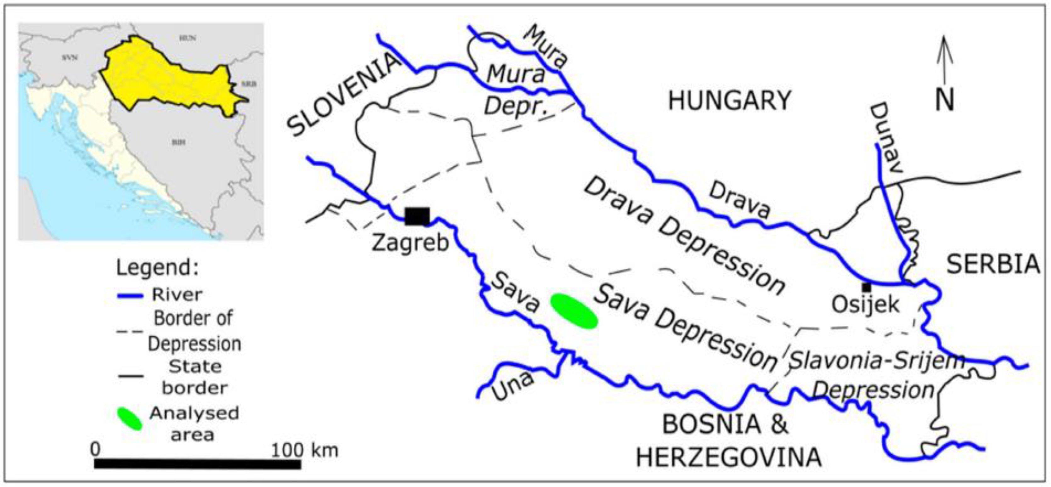
Figure 1. The location of field “B” in the Sava Depression (from [3]).
Stats 03 00007 g001
Figure 2. A structural map of the Late Miocene (Lower Pontian) reservoir “K”.
Stats 03 00007 g002
Figure 3. Correlation section through wells J-167–J-25alfa–J-166–J-149 shown on Figure 2 with reservoir boundaries marked by blue line (from [18]).
Stats 03 00007 g003
Figure 4. A sample of typical Middle Miocene (Badenian) calcarenite from northern Croatia (Breznički Hum locality). Collection of the Faculty of Mining, Geology and Petroleum Engineering.
Stats 03 00007 g004
Figure 5. A photomicrograph of the typical Middle Miocene (Badenian) calcarenite from northern Croatia (Breznički Hum locality), stained with alizarin red.
Stats 03 00007 g005
Figure 6. Points included within the IDW interpolation area (from [3]).
Stats 03 00007 g006
Figure 7. Radii of coverage of the MSM (modified from [3]).
Stats 03 00007 g007
Figure 8. Porosity of reservoir “K”: (a) IDW; (b) MSM.
Stats 03 00007 g008
Figure 9. Permeability of reservoir “K”: (a) IDW; (b) MSM.
Stats 03 00007 g009
Figure 10. Thickness of reservoir “K”: (a) IDW; (b) MSM.
Stats 03 00007 g010
Table 1. Descriptive statistics of geological variables porosity, permeability and thickness data in the “K” reservoir.
DescriptionNo DataMinMaxMean
Porosity190.2170.3150.232
Permeability (10−9 m2)1829.6121.285.7
Thickness (m)141247.7
Table 2. Raw data of porosity, permeability and thickness data interpolated in the “K” reservoir (coordinates are in a Gauss–Krueger system).
Well’s
No.
Surface XSurface YPorosity
(Parts of Unit)
Thickness
(m)
Permeability
(mD)
J-1016,421,0965,028,8770.2171121.2
J-1206,420,6585,029,0680.27215.729.6
J-1616,420,9575,028,8700.217329.6
J-1626,421,0345,028,5930.2176.5121.2
J-1676,420,5295,028,6740.21714.8121.2
J-1686,420,6995,028,4750.3151121.2
J-1696,420,7245,028,8250.21718.4121.2
J-1706,420,3495,028,9260.223729.6
J-1746,421,2985,028,8630.2171.129.6
J-1756,420,4755,029,1360.2233.2121.1
J-1586,420,3035,028,9100.2237.329.6
J-1716,420,5765,028,9700.2232429.6
J-1726,420,9285,029,1470.2230.529.6
J-1026,421,2085,028,9260.217 121.2
J-1486,421,1265,028,4370.217
J-1496,420,9595,028,5010.217 121.2
J-1666,420,7715,028,6500.217 121.2
J-256,420,5465,028,4600.3153.8121.2
J-1736,420,5395,028,3820.217 121.2
Table 3. Summary results of application of the IDW and MSM methods in reservoir "K".
DescriptionNo DataCross-Validation
Inverse Distance (IDW)Modified Shepard’s Method (MSM)
Porosity190.001190.00345
Permeability18480.8516.1
Thickness1440.760.5
Table 4. Recommended interpolation methods for small input data set [3].
Number of DataApplicability of Interpolation Method
Inverse Distance WeightingNearest NeighbourhoodNatural Neighbour
1–5YesYesNo
6–10YesYesYes
11–19YesYesYes
Table 5. Recommended choice between the IDW and MSM methods for a small input data set (less than 20 points of data.
Number of DataApplicability of Interpolation Method
Inverse Distance WeightingModified Shepard’s Method
Criteria
(1)
If the Nearest Neighbourhood, the Natural Neighbour or any available zonal method is tested and the IDW has the smallest cross-validation.
(2)
If other non-zonal methods are used, but cross-validation is a single criterion for a quick-look.
(1)
If IDW has a smaller cross-validation than the MSM, but the outliers are strongly and unnaturally emphasised on the map (“bull-eye”, “butterfly” features).
(2)
If the MSM is chosen, an expert geologist, with knowledge about the regional geology of the mapped volume must evaluate the map(s).
5–20YesYes