Abstract
We propose a parameter estimation method for non-stationary Poisson time series with the abnormal fluctuation scaling, known as Taylor’s law. By introducing the effect of Taylor’s fluctuation scaling into the State Space Model with the Particle Filter, the underlying Poisson parameter’s time evolution is estimated correctly from given non-stationary time series data with abnormally large fluctuations. We also developed a discontinuity detection method which enables tracking the Poisson parameter even for time series including sudden discontinuous jumps. As an example of application of this new general method, we analyzed Point-of-Sales data in convenience stores to estimate change of probability of purchase of commodities under fluctuating number of potential customers. The effectiveness of our method for Poisson time series with non-stationarity, large discontinuities and Taylor’s fluctuation scaling is verified by artificial and actual time series.
1. Introduction
The Poisson process is a basic stochastic process for events that occur at random in various natural and social phenomena, such as the number of decay of radioactive atoms, the occurrence of a failure of elements in devices, and daily sales amount of commodities []. As the Poisson process is fully described by just one parameter, , the mean value of events in a unit time, precise estimation of for a given data set is the key to understand the process.
Estimation of is an easy task if the data holds stationarity, as is given simply by the average number in a unit time. However, for any real system, we encounter the following two difficulties.
The first difficulty comes from non-stationarity. A wide variety of natural and social phenomena exhibit non-stationarity. The fluxes of cosmic radiation, such as active galactic nuclei and X-ray, are non-stationary on long time scales []. Insect population shows non-stationarity by the factors such as environmental changes and dynamics of the ecological system []. As for social phenomena, web page visitations, highway traffic [] and the underlying demand for a commodity [] changes non-stationarily by various uncontrollable factors like human activity, social trend and environmental condition. Thus, a time series in real systems generally shows complicated non-stationarity which is often unpredictable. Especially, in the case that the time scale of change of is short including discontinuous jumps, it is very difficult to estimate by the conventional methods such as the Poisson regression method [].
The second difficulty relates to the abnormally large fluctuations whose standard deviation is proportional to , while the width of fluctuation of the Poisson process is known to be given by . Taylor found the power law [] between the fluctuation and the mean value in observing the number of individuals in the ecosystem. This fluctuation scaling, known as Taylor’s law, has been confirmed in a variety of natural and social phenomena [], such as biology [], financial market [], networks [], frequencies of word appearances on internet blogs [] and sales []. The mechanism of the fluctuation scaling is known as follows. The basic process follows a Poisson process with a constant , but there exists fluctuation in the population of the observing objects, that gives the standard deviation of fluctuation proportional to the mean value, [,,,]. This fluctuation scaling is unavoidable in many cases since the total number of the observing objects is practically uncontrollable in the real system. For precise estimation of we have to distinguish the variation of by this effect from a non-stationary temporal change of . However, Taylor’s fluctuation scaling has not been attracted attention in the Poisson parameter estimation.
Non-stationary parameter estimation methods have been widely studied, such as Auto Regressive Integrated Moving Average (ARIMA) [], Neural Networks (NN) [], which are suitable for non-stationarity with regularity characterized by autocorrelations. Generalized Additive Model (GAM) [] can reveal the general trend of a non-stationary time series by fitting a smooth curve which is differentiable. The State Space Model (SSM) [] is applicable for unpredictable non-stationarity with abrupt and indifferentiable changes, therefore in this paper we generalize this method to handle non-stationary Poisson time series with Taylor’s fluctuation law.
In Section 2, we explain our method with short reviews of the non-stationary time series analyses to be used in our method. In Section 3, we verify our method by some artificial Poisson time series. In Section 4, we examine the effectiveness for actual data, namely Point-of-Sales (POS) data which shows non-stationarity and the fluctuation scaling with unpredictable sudden jumps.
2. Methods
2.1. Non-Stationary Time Series Analysis
A time series analysis method suitable for non-stationary cases, the State Space Model (SSM) [] is adopted in our method. In this subsection, we explain the SSM.
The SSM assumes that an observation value at time t is generated stochastically by an invisible state , where is stochastically determined depending on .
where denotes the Probability Density Function (PDF) of A conditioned by B, and the tilde (∼) in the formula, denotes that C is a stochastic variable following the PDF.
Equation (1) is called the system model in the SSM, which describes stochastic time evolution of the state . Equation (2) is called the observation model in the SSM, which defines the stochastic generation of the observation value from the state.
Non-stationarity of the Poisson mean value can be modeled in the system model Equation (1), regarding as the state . We define the system model as follows:
where m, , are hyper parameters. is the Normal distribution with the mean value equals to zero and the standard deviation equals to (). is the truncated Uniform distribution with the range from − to (). m characterizes the ratio of superposition of two distributions, the Normal and truncated Uniform distributions (). Equation (5) means that the stochastic time evolution of the change of generally follows either the Normal distribution with probability or the Uniform distribution with range of with probability m. The value of is determined as the range of the Uniform distribution is much larger than the fluctuation of the Normal distribution (), that allows a large change of . The superposition of two distributions considers the case where generally follows the Normal distribution, but sometimes changes up to with a small probability m. This kind of system model with long tail distribution allows better trackability of a non-stationarity. A system model defined by the superposition of a Normal distribution and a truncated Uniform distribution is already proposed by Yura et al. [] for non-stationary time series analysis of financial market data. Here, in our model the value of is limited to be non-negative by Equation (4) as the Poisson parameter (or ) needs to be positive.
The hyper parameters are to be determined in accordance with non-stationarity of Poisson for each system. We adopted , and by examining Root Mean Squared Error of estimation of some artificial time series, such as stationary, step-like and continuous rising. is Taylor’s fluctuation term to be described in the next subsection, Equation (6). The detailed information on the hyper parameters determination is provided in the Appendix A.
2.2. Taylor’s Fluctuation Scaling Law
The standard deviation of a Poisson process with Taylor’s fluctuation scaling, which is caused by the fluctuation in the population of the observing objects, is generally given as follows []:
Here, the proportional constant characterizes the strength of fluctuation of population and its value is determined by examining the relationship between the standard deviation and the mean of an actual data.
As an example, we explain a case of Point-of-Sales (POS) data. The POS data is taken from 243 chain stores of a major convenience store company in Japan during the 153 days from 1 June to 31 October 2010. We obtained daily sales time series of each product in each store from the POS data.
Figure 1 illustrates Taylor’s fluctuation scaling of sales data of a product (a soft drink). The solid line indicates where = 0.12, the dot-dash line is and the dashed line shows . Figure 1 is obtained by the following procedures.
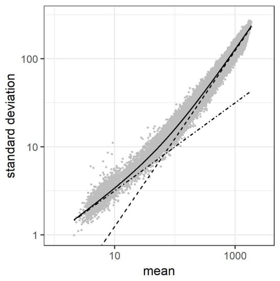
Figure 1.
Example of Taylor’s fluctuation scaling for daily sales number of a soft-drink in convenience stores. The mean values and the standard deviations are plotted for various data sets with different number of aggregated stores (49,924 points are plotted). Dot-dash line: , Dashed line: , Solid line: , where = 0.12.
- For small mean values we prepare data sets of daily sales numbers of the product for each store with specification by the day of the week (For example, sales number in every Monday). 243 (stores) × 7 (days of the week) = 1701 points are plotted.
- For larger mean values we prepare aggregated data sets by random sampling as follows. For each given number of stores, k, we choose k stores at random and the sales numbers are summed up for each day of the week. The value of k is from 2 to 243 and we repeat this procedure 30 times for each k (48,223 points are plotted.)
2.3. SSM of Our Method
We incorporate Taylor’s fluctuation scaling term into the SSM. The observation model Equation (2) for the Poisson process can be written as follows:
where is the Poisson distribution with the mean value . The observation value are generated stochastically by the distribution. Here, is stochastically determined by Equations (3)–(5).
In order to incorporate Taylor’s fluctuation scaling term Equation (6) as the standard deviation of Equation (7), we approximate the Poisson distribution by the Normal distribution in the case that is statistically large (i.e., ). The Normal distribution for and is very similar to the Poisson distribution for , and for , the distributions are virtually indistinguishable []. We apply the approximation by the normal distribution for since the skewness of the Poisson distribution of is smaller than that of , hence, closer to 0, which is the value of skewness of the normal distribution, whereas the ratio of change of the standard deviation by Taylor’s fluctuation scaling at is below , where .
2.4. Particle Filter
Our SSM contains non-Gaussian distribution such as the Poisson distribution and the truncated Uniform distribution. The Particle Filter algorithm [,] has the capability to solve such a non-Gaussian SSM.
The Particle Filter is a kind of Monte Carlo simulation which approximates a PDF of the state as the distribution of Monte Carlo sample values. Owing to the property of the Monte Carlo simulation, an arbitrary distribution function can be represented. The Monte Carlo samples are referred to as the particles in the Particle Filter. The distribution of the particles is updated by the observation value for each time t with the likelihood function. The set of the particles at time t conditioned by an observation value at time k is written in the form of , where N is the Monte Carlo sample size. The specific procedure of the Particle Filter which corresponds to the simulation code is as follows,
- Generate initial N particles and set .
- At time t:
- (a)
- (b)
- Using the observation value , estimate likelihood for each particle by Equation (9)
- (c)
- Update particles by resampling with the replacement of . The resampling probabilities for each particle are proportional to the likelihood of each particle.
- (d)
- If time t is the last step, stop the procedure. Otherwise, increment t and go to step 2 (a).
In this research, the number of Monte Carlo samples is set to N = 10,000 and the initial particles are generated by Equations (3)–(5) assuming for simplicity. We obtain a value for each time t by calculating the median, instead of mean, of the Monte Carlo samples of since its robustness against variations of particle values.
The Markov Chain Monte Carlo (MCMC) method [] is another candidate to solve our SSM. We selected the Particle Filter since it can solve the SSM stably even with a small amount of data.
2.5. Particle Filter with Discontinuity Detection
Our SSM introduce a wide range of Uniform distribution to follow large parameter changes in time series as shown in Equation (5). Moreover, we consider the cases that include discontinuous jump points at which time series value changes more than the range of the Uniform distribution.
Simply widening the range of the Uniform distribution results in reducing the density of the particles and increasing Monte Carlo error. We propose the following discontinuity detection and estimation correction method.
- Detect a discontinuous point by checking whether the observation value is out of the bound of the particle distribution.
- If a discontinuous point is detected, initialize the particle distribution with the observation value at the discontinuous point.
Using the observation value itself at the discontinuous point as the median of the particle distribution leads to overfit the data. We adopt or at the upward or downward discontinuous point respectively. Accordingly, the threshold of discontinuous point detection is set to be the upper bound + or lower bound − of the particle distribution.
We modify the algorithm of the Particle Filter shown in Section 2.4, step 2 (b) as follows,
- Generate initial N particles , set .
- At time t:
- (a)
- (b)
- If the observation value is above the upper bound or below the lower bound of the prediction distribution, go to step 1 and set to or at the upward or downward discontinuous point respectively. Otherwise, using the observation value , estimate likelihood for each particle by Equation (9) and go to next step .
- (c)
- Update particles by resampling with the replacement of . The resampling probabilities for each particle are proportional to the likelihood of each particle.
- (d)
- If time t is the last step, stop the procedure. Otherwise, increment t and go to step 2 (a).
2.6. Summary of the Parameter Estimation Procedure
We summarize the parameter estimation procedure. Steps 1 and 2 are preparations, and step 3 is the actual parameter estimation step.
- Estimate the proportional constant of Taylor’s fluctuation scaling by some previous data, as explained in Section 2.2.
- Apply the Particle filter described in Section 2.4 and Section 2.5 to solve the SSM, and estimate Poisson parameter of a time series. Poisson parameter is estimated basically based on the likelihood for an observation data at each time t. When the discontinuous trend jump is detected as explained in Section 2.5, the value of is estimated based on the observation data. No extrapolation is done, namely, we do not estimate the parameter where there is no data.
3. Simulation Tests
In this section, we verify the validity of our method with artificial time series generated by random number simulation. The distribution of random numbers is the Poisson distribution for small , i.e., , otherwise the Normal distribution with Taylor’s fluctuation scaling term Equation (6) where . The value is typical for the Point-of-Sales data used in this research []. Random numbers with a specific distribution can be obtained by the inversion method [].
3.1. Validity for Non-Stationarity
First, we demonstrate our method without discontinuity point detection, which is described in Section 2.5. Figure 2a shows a continuous rising time series from to in gray line. In this figure, the assumed values of and the estimated values of are shown in dotted line and black line respectively. We can confirm that the estimated values of follows the non-stationary continuous rising trend of the assumed values of . The Root Mean Squared Error (RMSE) between the assumed values of () and the estimated values of (), standardized by at each time as shown in Equation (12), is .
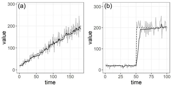
Figure 2.
Estimation results of two types of artificial non-stationary time series using the particle filter without discontinuous detection shown in Section 2.4. (a) Continuous rise time series from to 200. (b) Step-like time series from to 200. Gray line: artificial time series, Black dotted line: assumed values of , Black solid line: estimated values of .
Figure 2b indicates a step-like time series which increases from to 200 in gray line. The estimated values of in black line generally follows the abrupt step-like change of the assumed values of , but there exists some delay. The assumed values of changes 20 to 200 at time 50, but the estimated values of reaches to 200 at about time 80. The by Equation (12) is .
This delay is caused by the large discontinuity of the time series which is not covered by the range of the prediction distribution, that is, the range of the truncated uniform distribution in Equation (5). By introducing the discontinuous point detection as mentioned in Section 2.5, the delay is corrected as shown in Figure 3. The is improved to be .
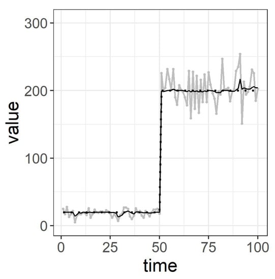
Figure 3.
Correction of estimated values of at the discontinuous point using the particle filter with discontinuous detection shown in Section 2.5. Gray line: artificial time series, Black dotted line: assumed values of , Black solid line: estimated values of .
3.2. Validity for Taylor’s Fluctuation Scaling
Figure 4a shows a step-like time series from to 640 increased by two times every 30 data points which is shown in gray line, and the estimated values of in black line. The is .
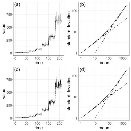
Figure 4.
Verification for Taylor’s fluctuation scaling with step-like time series from to 640. (a) Black solid line: estimated values of with our model, Gray line: artificial time series, Black dotted line: assumed values of (b) The mean and the standard deviation plots of (a). (c) Black solid line: estimated values of with conventional Poisson model, Gray line: artificial time series, Black dotted line: assumed values of . (d) The mean and the standard deviation plots of (c). In (b,d), Dot-dash line: , Dashed line: , Solid line: , where .
To verify the validity of the estimated values of , we examined the deviation of time series values from the estimated values of . If the estimated values are reasonable, the relationship between the standard deviation calculated with time series and should follow Equation (6). The specific procedure for calculating the standard deviation and the mean is as follows,
- Make pairs of estimated values of and time series value for each time t.
- Divide the pairs into groups by exponential bins such as for estimated values of values.
- Calculate the standard deviation with the time series value and estimated values of for each group. Obtain the mean with the estimated values of for each group.
The result is shown in Figure 4b. The plots are along the relationship of Taylor’s fluctuation scaling illustrated in black solid line. This ensures the validity of our model for Taylor’s fluctuation scaling. The RMSE between the theoretical standard deviation () by Equation (6) and the estimated standard deviation (), standardized by at each time as shown in Equation (13), is .
To clarify the advantage of our model to the conventional Poisson model, we performed an estimation of the same time series as in Figure 4a with the conventional Poisson model, that is, with Equation (7) instead of Equation (8). The results are shown in Figure 4c,d. One can see that the estimated values of time series in Figure 4c follows the fluctuation of the time series excessively. The conventional Poisson model regards large fluctuation caused by Taylor’s fluctuation scaling as variation of . Figure 4d illustrates that the Poisson model estimates the fluctuation as in dot-dash line, while the true fluctuation is Equation (6) in solid line. The is .
Along with the step-like time series, we examined the case of a continuous rising time series. Figure 5a,b are the estimated results by our method with Taylor’s fluctuation scaling term. The is . Figure 5c,d are the results by the conventional Poisson model. The is . These results also demonstrate the effectiveness of our method for estimating the Poisson with Taylor’s fluctuation scaling.
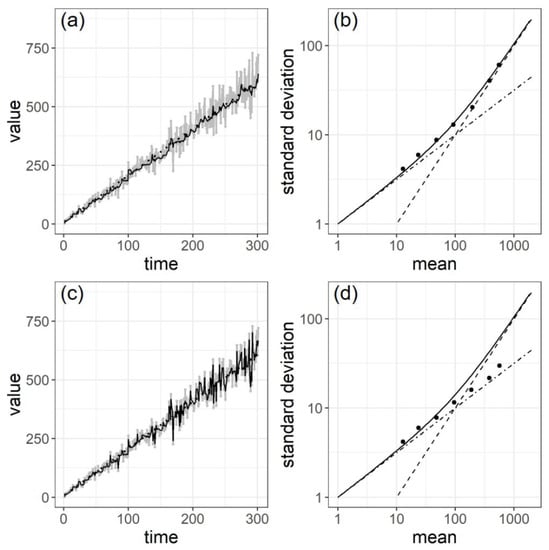
Figure 5.
Verification for Taylor’s fluctuation scaling with continuous rising time series from to 600. (a) Black solid line: estimated values of with our model, Gray line: artificial time series, Black dotted line: assumed values of . (b) The mean and the standard deviation plots of (a). (c) Black solid line: estimated values of with conventional Poisson model, Gray line: artificial time series, Black dotted line: assumed values of . (d) The mean and the standard deviation plots of (c). In (b,d), dot-dash line: , dashed line: , solid line: , where .
4. Point-of-Sales (POS) Data Tests
We verified our method by actual data, namely, the POS data described in Section 2.2. The POS data is a typical example of the non-stationary Poisson time series with Taylor’s fluctuation scaling [].
Figure 6a shows a daily sales number series of a product (an ice cream) at a store. One can see the arch-shaped trend in the sales time series in gray line, and the estimated values of in black line follows the trend. Figure 6b clarifies that the relationship between the mean and the standard deviation of the estimated values of values are along the relationship derived from Taylor’s fluctuation scaling Equation (6). The is .
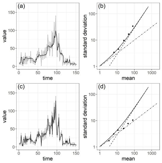
Figure 6.
Estimation results of an arch-shaped sales time series. (a) Gray line: sales time series, Black line: estimated values of with our model. (b) The mean and the standard deviation plots of (a). (c) Gray line: sales time series, Black line: estimated values of with conventional Poisson model. (d) The mean and the standard deviation plots of (c). In (b,d), dot-dash line: , dashed line: , solid line: , where (an ice cream) [].
Figure 6c,d show the estimation results of the same time series in Figure 6a, with the conventional Poisson model. The Poisson model results in overfitting of the to the time series as shown in Section 3.2. The is . The advantage of incorporating the term of Taylor’s fluctuation scaling in precise estimation of the Poisson parameter is confirmed with this actual data.
Figure 7a indicates a sales time series of a product (a meat bun) of a store which shows sudden rises at around time 10 and 52. The estimated values of in black line well follows the sudden rises. Figure 7b shows the estimated values of are along the relationship of Taylor’s fluctuation scaling. The is .
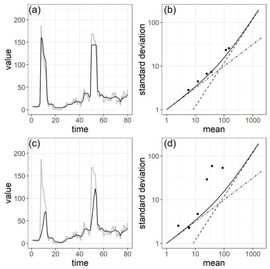
Figure 7.
Estimation results of a sales time series with discontinuity. (a) Gray line: sales time series, Black line: estimated values of with our model. (b) The mean and the standard deviation plots of (a). (c) Gray line: sales time series, Black line: estimated values of with our model without the correction method at discontinuous points. (d) The mean and the standard deviation plots of (c). In (b,d), dot-dash line: , dashed line: , solid line: , where (a fried item) [].
Figure 7c,d show the estimation results of the same time series in Figure 7a, without using the correction method at discontinuous points. We can find that the estimated values of in black line are underfitted to the time series in gray line at the large discontinuous points. The is . Thus, the merit of the correction method at discontinuous points is verified with the actual time series.
5. Conclusions
The effectiveness of our method of tracking the Poisson parameter for abnormally large fluctuation time series with non-stationarity is verified one by one with artificial time series. We revealed the advantage of our method considering the term of Taylor’s fluctuation scaling to the conventional Poisson model, namely, our model distinguishes non-stationarity of the parameter from the large fluctuation caused by this fluctuation scaling. We also presented the method of detecting discontinuity of the time series. By correcting estimation values at the discontinuous point in time series, we realized precise parameter estimation with non-stationary time series with large discontinuity. Along with some artificial time series, we verified the effectiveness of our method by some actual Point-of-Sales data which shows non-stationarity, large discontinuities and Taylor’s fluctuation scaling.
We assume the case that Taylor’s fluctuation scaling is generally caused by the fluctuation in the population of the observing objects, which leads the standard deviation to be proportional to Poisson mean value , namely, the scaling exponent becomes 1. The scaling exponent 1 is observed in many natural and social phenomena, such as cell numbers of species [], fluxes of cosmic radiation [], daily water-level of a river [], web page visitations [], highway traffic [] and sales [].
Considering effects other than fluctuation in the population, there are cases that the Taylor’s scaling exponent takes a value between 0.5 and 1.0 as we can find examples in POS data on stamps and magazines []. Stamps are often purchased in bulk, and magazines are specifically bought on the launch day. The purchase processes of these items are not regarded as a simple Poisson process, that leads to the scaling exponent under 1. The extension of the proposed model for more general Taylor’s fluctuation scaling is a potential future research task.
Periodicity in the time series, such as seasonality and circadian variation behind the daily data, are not considered in the present model. In practical applications in the future, applying the method to some cases such as trend forecast, an extension of our method taking into account such periodicity may yield better accuracy of the parameter estimation.
Our method deals with parameter estimation of a non-stationary Poisson time series of number of events observing with regular intervals in the case that the population is also changing randomly. Meanwhile, there exist methods based on Poisson point process suitable for describing events in discrete points in time. The Spatial Mixed Poisson Process(SMPP) [,,,,] is such an example, which can handle the case that the underlying random event is correlated to the observing event that is stochastically determined. The SMPP can model the delay of the impact from the underlying event to the observing event since both events are described separately in discrete points in time, which is suitable for application to rare but correlated events such as occurrence of cascading crashes in financial markets. There are wide variety of phenomena both in nature and in our society, which are considered to be described basically by a variant of Poisson process. More different approaches will appear in the near future to cope with the increasing big data in the society.
Author Contributions
Conceptualization, G.S., H.T. and M.T.; Data curation, G.S.; Formal analysis, G.S.; Funding acquisition, M.T.; Investigation, G.S.; Methodology, G.S., H.T. and M.T.; Project administration, H.T. and M.T.; Resources, M.T.; Software, G.S.; Supervision, H.T. and M.T.; Validation, G.S.; Visualization, G.S.; Writing—original draft, G.S.; Writing—review and editing, H.T. and M.T.
Funding
This work was partially supported by JSPS KAKENHI (Grant No.18H01656) and JST, Strategic International Collaborative Research Program (SICORP) on the topic of ”ICT for a Resilient Society” by Japan and Israel.
Acknowledgments
The authors would like to thank Seven-Eleven Japan Co.,Ltd. for providing the POS data.
Conflicts of Interest
The authors declare no conflict of interest.
Appendix A. Estimation of the Hyper Parameters
Equation (5) contains three hyper parameters, m, and . We determined the value of each parameter by the following procedure. We assumed three types of time series, stationary as shown in Figure A1a, discontinuous step-like change as illustrated in Figure A2a and continuous rise as indicated in Figure A3a. We generated 100 sets of random number time series for each three types by random number simulation mentioned in Section 3. We estimate time series for each time series and examined Root Mean Squared Error (RMSE) of estimated and assumed values of by changing m, , . The proportional constant of the fluctuation scaling is assumed 0.1, which is typical for the Point-of-Sales data used in this research []. The is assumed in the form of , where is Taylor’s fluctuation scaling term Equation (6), meaning that the range of the Uniform distribution in Equation (5) is determined based on the variance by Equation (6) at each .
The results for stationary time series is shown in Figure A1b–d. One can see that small RMSE for stationary time series is obtained when the value of each parameter, m, and are small. It is reasonable because small m, and lead to a narrow prediction distribution and less sensitivity to variations in a stationary time series.
The results for step-like change shown in Figure A2 are almost opposite parameter dependencies to Figure A1 since a wide prediction distribution contributes to sensitiveness to the change. One should note that a prediction distribution wider than necessary results in large RMSE because of the Monte Carlo error. The results for continuous rise in Figure A3 shows generally similar parameters dependence as Figure A2, in the cases of too small or too large m, and result in large RMSE.
We adopted , and , marked with yellow rectangles in Figure A1, Figure A2 and Figure A3 , since these are one of the balanced condition giving small RMSE for three types of time series examined.

Figure A1.
RMSE result of stationary time series. (a) An example of the stationary time series. Gray line: artificial time series, Black dotted line: assumed values of . (b) m = 0.05, where m is the ratio of the Uniform distribution to the Normal distribution, (c) m = 0.10, (d) m = 0.15. The yellow square shows the parameter sets we adopted in our simulation and real data analysis.

Figure A2.
RMSE result of non-stationary, step-like time series. (a) An example of the step-like time series. Gray line: artificial time series, Black dotted line: assumed values of . (b) m = 0.05, (c) m = 0.10, (d) m = 0.15. The yellow square shows the parameter sets we adopted in our simulation and real data analysis.

Figure A3.
RMSE result of non-stationary, continuous rising time series. (a) An example of the continuous rising time series. Gray line: artificial time series, Black dotted line: assumed values of . (b) m = 0.05, (c) m = 0.10, (d) m = 0.15. The yellow square shows the parameter sets we adopted in our simulation and real data analysis.
The hyper parameters in the SSM can be adjusted by using self-organizing state space model []. The proposed method is for tracking a non-stationary change even at the initial stage of a time series (i.e., ) where sample size for the adjustment is not enough. For the stability of the estimation, the value of each hyper parameters is determined as described above.
References
- Fukunaga, G.; Takayasu, H.; Takayasu, M. Property of Fluctuations of Sales Quantities by Product Category in Convenience Stores. PLoS ONE 2016, 11, e0157653. [Google Scholar] [CrossRef] [PubMed]
- Azevedo, R.B.R.; Leroi, A.M. The flux-dependent amplitude of broadband noise variability in X-ray binaries and active galaxies. Mon. Not. R. Astron. Soc. 2001, 323, L26–L30. [Google Scholar]
- Turchin, P.; Taylor, A.D. Complex Dynamics in Ecological Time Series. Ecology 1992, 73, 289–305. [Google Scholar] [CrossRef]
- De Menezes, M.A.; Barabási, A.-L. Separating Internal and External Dynamics of Complex Systems. Phys. Rev. Lett. 2004, 93, 068701. [Google Scholar] [CrossRef] [PubMed]
- Winkelmann, R. Econometric Analysis of Count Data; Springer: Berlin/Heidelberg, Germany, 2008; pp. 63–126. [Google Scholar]
- Taylor, L.R. Aggregation, variance and the mean. Nature 1961, 189, 732–735. [Google Scholar] [CrossRef]
- Eisler, Z.; Bartos, I.; Kertész, J. Fluctuation scaling in complex systems: Tayolr’s law and beyond. Adv. Phys. 2008, 57, 89. [Google Scholar] [CrossRef]
- Kendal, W.S. A frequency distribution for the number of hematogenous organ metastases. J. Theor. Biol. 2002, 217, 203–218. [Google Scholar] [CrossRef]
- Eisler, Z.; Kertész, J. Scaling theory of temporal correlations and size-dependent fluctuations in the traded value of stocks. Phys. Rev. E. 2006, 73, 046109. [Google Scholar] [CrossRef]
- De Menezes, M.A.; Barabási, A.-L. Fluctuations in network dynamics. Phys. Rev. Lett. 2004, 92, 028701. [Google Scholar] [CrossRef]
- Sano, Y.; Yamada, K.; Watanabe, H.; Takayasu, H.; Takayasu, M. Empirical analysis of collective human behavior for extraordinary events in the blogosphere. Phys. Rev. E. 2013, 87, 012805. [Google Scholar] [CrossRef]
- Meloni, S.; Gomez-Gardeñes, J.; Latora, V.; Moreno, Y. Scaling Breakdown in Flow Fluctuations on Complex Networks. Phys. Rev. Lett. 2008, 100, 208701. [Google Scholar] [CrossRef] [PubMed]
- Box, G.; Jenkins, G. Time Series Analysis: Forecasting and Control; Holden-Day: San Francisco, CA, USA, 1976. [Google Scholar]
- Zhang, G.P. Neural Networks for Time-Series Forecasting, Handbook of Natural Computing; Springer: Berlin/Heidelberg, Germany, 2012; pp. 461–477. [Google Scholar]
- Hastie, T.; Tibshirani, R. Generalized Additive Models; Chapman and Hall: London, UK, 1990. [Google Scholar]
- Harvey, A. Forecasting with Unobserved Components Time Series Models, Handbook of Economic Forecasting; Elsevier: Amsterdam, The Netherlands, 2006. [Google Scholar]
- Yura, Y.; Takayasu, H.; Nakamura, K.; Takayasu, M. Rapid Detection of the Switching Point in a Financial Market Structure Using the Particle Filter. J. Stat. Comput. Simul. 2014, 84, 2073–2090. [Google Scholar] [CrossRef]
- Watanabe, H.; Sano, Y.; Takayasu, H.; Takayasu, M. Statistical properties of fluctuations of time series representing appearances of words in nationwide blog data and their applications: An example of modeling fluctuation scalings of nonstationary time series. Phys. Rev. E 2016, 94, 052317. [Google Scholar] [CrossRef]
- Draper, N.R.; Smith, H. Applied Regression Analysis; Wiley: Hoboken, NJ, USA, 1998; pp. 505–565. [Google Scholar]
- Cherry, S.R.; Sorenson, J.A.; Phelps, M.E. Physics in Nuclear Medicine, 4th ed.; Elsevier: Amsterdam, The Netherlands, 2012; pp. 126–128. [Google Scholar]
- Kitagawa, G. Monte Carlo Filter and Smoother for Non-Gaussian Nonlinear State Space Models. J. Comput. Graph. Stat. 1996, 5, 1–25. [Google Scholar]
- Gordon, N.J.; Salmond, D.J.; Smith, A.F. Novel approach to nonlinear/non-Gaussian Bayesian state estimation. IEE Proc. F-Radar Signal Process. 1993, 140, 107–113. [Google Scholar] [CrossRef]
- Liu, J.S. Monte Carlo Strategies in Scientific Computing; Springer: Berlin, Germany, 2001. [Google Scholar]
- Luc, D. Non-Uniform Random Variate Generation; Springer: Berlin/Heidelberg, Germany, 1986; pp. 27–36. [Google Scholar]
- Azevedo, R.B.R.; Leroi, A.M. A power law for cells. Proc. Natl. Acad. Sci. USA 2001, 98, 5699–5704. [Google Scholar] [CrossRef] [PubMed]
- Jánosi, I.M.; Gallas, J.A.C. Growth of companies and water-level uctuations of the river Danube. Physica A 1999, 271, 448–457. [Google Scholar] [CrossRef]
- Cerqueti, R.; Fenga LVentura, M. Does the U.S. exercise contagion on Italy? A theoretical model and empirical evidence. Physica A 2018, 499, 436–442. [Google Scholar] [CrossRef]
- Cerqueti, R.; Ventura, M. Risk and Uncertainty in the Patent Race: A Probabilistic Model. IMA J. Manag. Math. 2015, 26, 39–62. [Google Scholar] [CrossRef]
- Cerqueti, R.; Ventura, M. Patent Valuation Under Spatial Point Processes with Delayed and Decreasing Jump Intensity. BE J. Theor. Econ. 2015, 15, 433–456. [Google Scholar] [CrossRef]
- Cerqueti, R. Exhaustion of Resources: A Marked Temporal Process Framework. Stoch. Environ. Res. Risk Assess. 2014, 28, 1023–1033. [Google Scholar] [CrossRef]
- Cerqueti, R.; Foschi, R.; Spizzichino, F. A Spatial Mixed Poisson Framework for Combination of Excess of Loss and Proportional Reinsurance Contracts. Insur. Math. Econ. 2009, 45, 59–64. [Google Scholar] [CrossRef]
- Kitagawa, G. A self-organizing state-space model. J. Am. Stat. Assoc. 1998, 93, 1203–1215. [Google Scholar] [CrossRef]
© 2019 by the authors. Licensee MDPI, Basel, Switzerland. This article is an open access article distributed under the terms and conditions of the Creative Commons Attribution (CC BY) license (http://creativecommons.org/licenses/by/4.0/).