One-Parameter Weibull-Type Distribution, Its Relative Entropy with Respect to Weibull and a Fractional Two-Parameter Exponential Distribution

Abstract

A new one-parameter distribution is presented with similar mathematical characteristics to the two parameter conventional Weibull. It has an estimator that only depends on the sample mean. The relative entropy with respect to the Weibull distribution is derived in order to examine the level of similarity between them. The performance of the new distribution is compared to the Weibull and in some cases the Gamma distribution using real data. In addition, the Exponential distribution is modified to include an extra parameter via a simple transformation using fractional mathematics. It will be shown that the modified version also exhibits Weibull characteristics for particular values of the second parameter.

1. Introduction

A one-parameter distribution is presented, hereby referred to as the 1D-Weibull, which has asymptotic behaviour similar to the conventional Weibull. Unlike the two parameter formulation of the latter, the 1D-Weibull only has one parameter, w, bounded by the interval $0\le w\le 1$. The estimator of this parameter depends only on the sample mean. Distributions like the Weibull generally have two or more parameters in order to characterise the statistical behaviour of physical phenomena. This presents a number of issues such as the fact that estimating two or more parameters introduces greater loss associated with small or poor sampling during the estimation process. The question arises as to whether it is possible to reduce such losses by using ‘simple’ distributions with less parameters but with equally good performance. Thus, aside from introducing the 1D-Weibull as a stand-alone distribution, the paper will also examine whether the 1D-Weibull can be used as a one-parameter alternative to the Weibull. To answer this question, a metric is required that determines the degree of separation or relative entropy (divergence) between them. For small relative entropy the two-parameter Weibull can be replaced by the simpler one-parameter 1D-Weibull distribution. Under this condition, the 1D-Weibull is expected to perform at least as well as the two-parameter conventional Weibull distribution.

One reason why there is interest at finding distributions with a smaller number of parameters is because they don’t have issues of complexity and over-fitting. The simpler distribution with good performance is better for modelling purposes. This can be deduced from the Akaike information criterion (AIC) [1,2] and other variants such as the Bayesian information criterion when examining the performance between two distributions against data. The AIC was obtained by Akaike while seeking to find a connection between the relative entropy of information theory and the maximum likelihood method. When comparing a number of models against the same data, the model with the minimum AIC is the one preferred but the AIC includes a penalty for those models with more parameters in order to discourage over-fitting. This means that for two distributions that perform equally well against the same data the one with the smaller number of parameters will be the best model. The AIC gives an asymptotic estimate of the performance between distributions and only on the same data. It does not assume knowledge of the distribution that created the data. The AIC between the 1D-Weibull and Weibull will be compared in the paper. However, a more powerful analytic approach for comparing two distributions whose mathematical forms are known, regardless of whether the data is the same or not, is to calculate the relative entropy between them.

The relative entropy between the 1D-Weibull and Weibull distributions will be derived on the basis of the Kullback-Leibler (K-L) divergence formulation [3,4,5,6,7,8,9,10]. The Kullback-Leibler approach has been used previously to examine the separation between probability densities [11,12,13,14]. This has been done with the aim of replacing one standard version with another whenever the relative entropy between them is small or zero. The conventional relative entropy between two standard distributions, while of academic interest, serves no practical purpose in the analysis of real physical processes. This is due to the fact that the solutions which achieve small relative entropy between them are trivial or unique and might arise from intersections for example. Failure to obtain small or zero relative entropy between two distributions is mainly due to their different mathematical forms which are used for modelling specific problems. The requirement is to find distributions that have zero or very close to zero relative entropy with respect to more complicated distributions while also having a smaller number of parameters. In addition, a small relative entropy must be valid for a larger solution set beyond the unique or trivial cases. Only then is it useful to replace a complicated distribution with a simpler one.

The K-L relative entropy gives solutions which contain the parameters of the two densities. This allows testing of different estimators for all the parameters since the goal is to find estimators that minimise or set the relative entropy to zero. This will be seen later in the paper when it is shown that the estimator $\widehat{w}$ of the 1D-Weibull density is equivalent to $w_{min}$, derived from the expression for the relative entropy, that minimises the divergence between the 1D-Weibull and Weibull densities. In other words, the estimator $\widehat{w}$ obtained from the maximum likelihood method (MLM) is equivalent to the ‘theoretical’ expression $w_{min}$ which minimises the relative entropy between the 1D-Weibull and standard Weibull densities. Thus the latter approach can be explored as an alternative to the MLM for obtaining parameter estimators. In addition, the relative entropy allows easy determination of upper and lower bounds for such estimators. Under certain conditions, the relative entropy can be connected to the Fisher information matrix directly.

It it worth noting two ‘issues’ with the K-L formulation. The K-L is a pseudo-metric as it is not symmetric for large separations between the two densities and does not obey the triangle inequality. It is rather simple to make it symmetric for large separations however. If two probability densities $p\left(x\right)$ and $q\left(x\right)$ have relative entropy $D\left(p\right(x\left)\right|\left|q\right(x\left)\right)$, then their relative entropy can be made symmetric using the following expression

$$\begin{array}{c}\hfill D\left(p\right(x\left)\right|\left|q\right(x\left)\right)=D\left(p\right(x\left)\right|\left|q\right(x\left)\right)+D\left(q\right(x\left)\right|\left|p\right(x\left)\right)\end{array}$$

(1)

The relative entropy has a mathematical duality with the Fisher-Rao geodesic which is symmetric for all separations and obeys the triangle inequality [15]. This is especially true in the limit of small separation between the two densities. For almost all cases of interest however, the issues of symmetry and large separation of densities are of no consequence.

In addition to deriving distributions with reduced parameters such as the 1D-Weibull, it is possible to increase the number of parameters too. For instance, a standard distribution such as the Exponential which has decaying characteristics, can be modified to include an extra parameter. The (fractional) two-parameter Exponential distribution will also be presented which contains the standard Exponential decaying characteristics as a special limit of the second parameter. It also has performance that is analogous to the standard Weibull and extreme-value type distributions. It will be shown that via the use of fractional mathematics, a simple transformation can be obtained that makes this possible. The transformation takes a random variable x and transforms it to a form that is a function of the second parameter. This parameter $\alpha$ is the fractional order appearing in the transformation. The fractional order is inherent in the operators which are used in fractional differentiation and integration. Fractional mathematics has the potential to change the way statistical analysis of problems is made. The reader is referred to [16,17,18] for details and the references therein. It is worth noting that the word ‘fractional’ is a historical misnomer. The term ‘fractional’ mathematics should in fact be understood to mean ‘generalised’ mathematics. For example integer order differentiation and integration are special limits of the fractional (general) versions.

Firstly however, the 1D-Weibull distribution is considered and its performance against the conventional two-parameter Weibull is investigated theoretically and later in Section 5 on real data.

2. The 1D-Weibull Distribution and Its Statistical Properties

The conventional Weibull distribution is parametrised by a shape parameter k and scale parameter $\lambda$ such that the CDF is given by

$$\begin{array}{c}\hfill {\tilde{\rho }}_0\left(x\right)=1-e^{-\frac{x^k}{{\lambda }^k}}\end{array}$$

(2)

and the PDF is given by the derivative of the CDF which becomes

$$\begin{array}{c}\hfill {\rho }_0\left(x\right)=\frac{k}{{\lambda }^k}{x}^{k-1}{e}^{-\frac{x^k}{{\lambda }^k}}\end{array}$$

(3)

It is worth pointing out that when the Weibull shape parameter takes the value $k=1$, the asymptotic performance of the Weibull distribution behaves like the exponential distribution. The case when $k=2$ is a very special limit and the Weibull reduces to the Rayleigh distribution. Finally when $k=3.5$, the asymptotic behaviour of the Weibull distribution resembles a Gaussian or Normal distribution. Generally, in order to model a physical system, both of the parameters k and $\lambda$ are required. These parameters can be estimated by sampling observed data sets. Using the maximum likelihood approach an estimator for $\widehat{k}$ can be obtained as:

$$\begin{array}{c}\hfill \frac{1}{\widehat{k}}=\frac{{\sum }_{i=1}^n{x}_i^{\widehat{k}}log\left(x_i\right)}{{\sum }_{i=1}^n{x}_i^{\widehat{k}}}-\frac{1}{n}\sum _{i=1}^{n}log\left(x_i\right)\end{array}$$

(4)

Given the form of the estimator for k, (4) must be solved numerically. The estimator for $\widehat{\lambda }$ is obtained via a simpler expression,

$$\begin{array}{c}\hfill {\widehat{\lambda }}^k=\frac{1}{n}\sum _{i=1}^n{x}_i^k\end{array}$$

(5)

where the total number of variables sampled is n. In order to obtain $\lambda$ in (5), the shape parameter k has to be estimated first using (4).

A one-parameter Weibull distribution which has asymptotic behaviour that is similar to the two-parameter Weibull distribution is now considered. The one parameter Weibull-type distribution (1D-Weibull) has parameter w whose estimator is obtained from the sample mean. The CDF is given as

$$\begin{array}{c}\hfill \tilde{\rho }\left(x\right)=1+w^x\left[\frac{2+log\left(w\right)\left[x(x+1)log\left(w\right)-2x-1\right]}{log\left(w\right)-2}\right]\end{array}$$

(6)

The density (PDF) is given as the derivative of (6) so that:

$$\begin{array}{c}\hfill \rho \left(x\right)=\frac{d\tilde{\rho }\left(x\right)}{dx}\equiv \frac{{log}^3\left(w\right)}{log\left(w\right)-2}x(x+1)w^x\end{array}$$

(7)

Both the CDF (6) and PDF (7) depend only on one parameter w whose values are bounded in the interval $0\le w\le 1$. The following limits apply to the PDF:

$$\begin{array}{c}\hfill \underset{x\to 0}{lim}\rho \left(x\right)=0;\underset{x\to \infty }{lim}\rho \left(x\right)=0\end{array}$$

(8)

and

$$\begin{array}{c}\hfill \underset{x\to 0}{lim}\tilde{\rho }\left(x\right)=0;\underset{x\to \infty }{lim}\tilde{\rho }\left(x\right)=1\end{array}$$

(9)

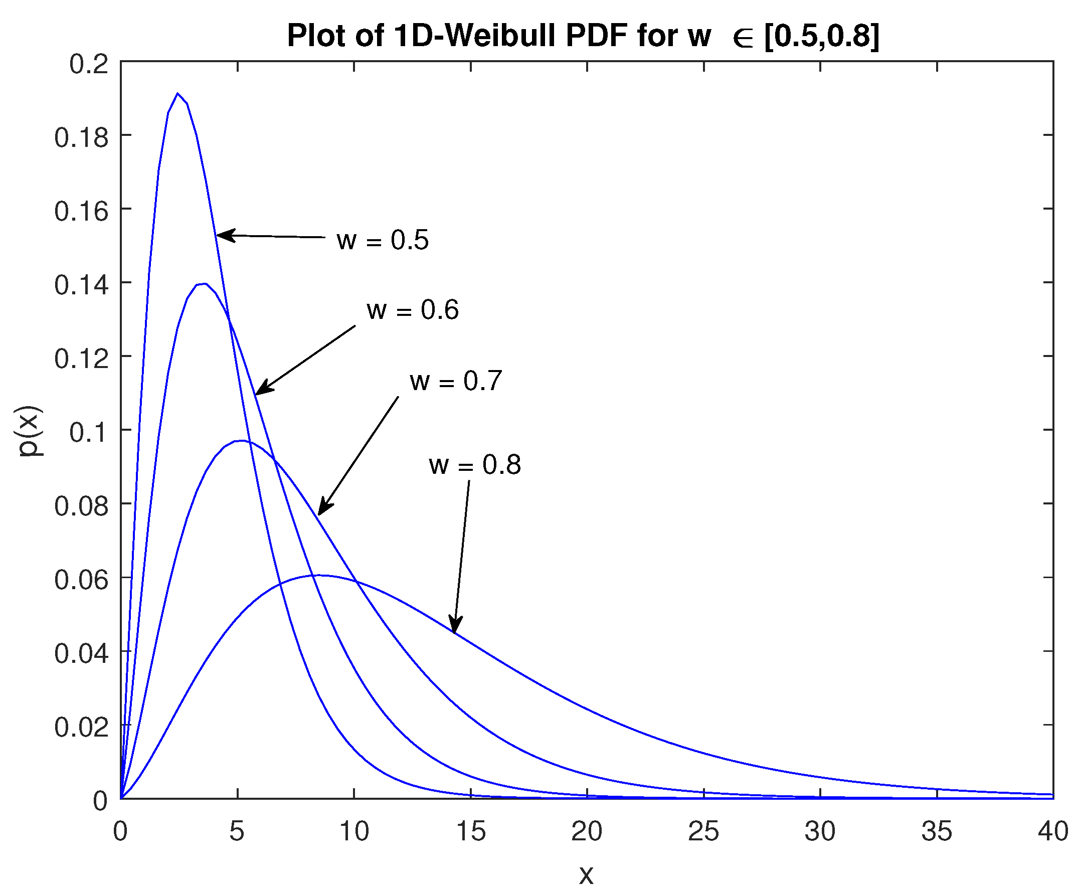
for the CDF. Figure 1 shows plots of the density for varying w values. The behaviour of the 1D-Weibull distribution is analogous to the two parameter Weibull. How much so will require a separation metric or divergence that can determine the degree of separation (or similarity) between them. This will be done in the context of the relative entropy in the next Section but before that, some important statistical properties of the 1D-Weibull distribution will be derived. An estimator $\widehat{w}$ can be obtained from the maximum likelihood method. Let the likelihood function be

$$\begin{array}{c}\hfill l\left(w\right)=\prod _{i=1}^n\frac{{log}^3\left(w\right)}{log\left(w\right)-2}{x}_i(x_i+1)w^{x_i}\end{array}$$

(10)

The log-likelihood of (10) is expanded as follows where the left hand side is written as $L\left(w\right)=log\left(l\right(w\left)\right)$:

$$\begin{array}{c}\hfill L\left(w\right)=log\left(\frac{{log}^{3n}\left(w\right)}{{(log\left(w\right)-2)}^n}\right)+\sum _{i=1}^{n}log\left(x_i\right)+\sum _{i=1}^{n}log(x_i+1)+log\left(w\right)\sum _{i=1}^n{x}_i\end{array}$$

(11)

The estimator $\widehat{w}$ can be obtained by taking the derivative of (11) and setting it to zero,

$$\begin{array}{ccc}\hfill \frac{\partial }{\partial w}L\left(w\right)& =& \frac{3n}{wlog\left(w\right)}-\frac{n}{w(log(w)-2)}+\frac{1}{w}\sum _{i=1}^n{x}_i\hfill \\ & \equiv & 0\hfill \end{array}$$

(12)

By simplifying (12), it is shown that the estimator is easily obtained via the quadratic equation:

$$\begin{array}{c}\hfill {log}^2\left(w\right)+\frac{2(1-\mu )}{\mu }log\left(w\right)-\frac{6}{\mu }=0\end{array}$$

(13)

where $\mu$ is the mean. The solution can be readily obtained via the use of the transformation $x=log\left(w\right)$ so that

$$\begin{array}{c}\hfill x^2+\frac{2(1-\mu )}{\mu }x-\frac{6}{\mu }=0\end{array}$$

(14)

As expected from a quadratic equation, there are two solutions such that

$$\begin{array}{c}\hfill x_{\pm }=\frac{1}{\mu }\left(\mu -1\pm \sqrt{{\mu }^2+4\mu +1}\right)\end{array}$$

(15)

The negative solution ensures that the estimator lies within the correct bounds $0\le \widehat{w}\le 1$. Thus using the definition of x, the following form is obtained for the estimator $\widehat{w}$:

$$\begin{array}{c}\hfill \widehat{w}=exp\left[\frac{1}{\mu }\left(\mu -1-\sqrt{{\mu }^2+4\mu +1}\right)\right]\end{array}$$

(16)

where $\mu$ can be either the population or sample mean respectively, i.e.,

$$\begin{array}{c}\hfill \mu =\frac{1}{n}\sum _{i=1}^n{x}_i\end{array}$$

(17)

and n is the total number of random variables sampled in the data. In order to test the convergence of the estimator $\widehat{w}$, i.e., (16), Monte Carlo simulations were performed using a seed value for w. The convergence of the estimator to the seed was tested and a typical result is shown in Figure 2.

In this example, $N=1000$ samples were generated randomly from the 1D-Weibull PDF each time for $N_{M.C.}=1\times {10}^4$ simulations. From Figure 2 the estimator for the 1D-Weibull distribution possesses the correct convergence. This is to be expected as the estimator $\widehat{w}$ depends on the sample mean. Thus the convergence of the estimator depends on the correct estimation of the mean of the randomly generated data samples. Next, the moments $<x^m>$ of the 1D-Weibull will be presented for $m=0,1,2,\dots$. The moments are obtained from,

$$\begin{array}{c}\hfill <x^m>={\int }_{\Omega }{x}^m\rho \left(x\right)dx\end{array}$$

(18)

where the 1D-Weibull density is given by (7) and the integration domain is $\Omega \in [0,\infty ]$. Specifically, the moments are calculated as:

$$\begin{array}{c}\hfill <x^m>=\frac{{log}^3\left(w\right)}{log\left(w\right)-2}{\int }_0^{\infty }{x}^{m+1}(x+1)w^{x}dx\end{array}$$

(19)

Expanding the integrand and using integration by parts yields the following result for the 1D-Weibull moments,

$$\begin{array}{c}\hfill <x^m>=\frac{\Gamma (m+2)\left(log\left(w\right)-m-2\right)}{{log}^m\left(w^{-1}\right)\left(log\left(w\right)-2\right)}\end{array}$$

(20)

Observe that the $m=0$ order gives $<x^0>=1$ which is also readily seen from (18), that is, the second axiom of probability is obtained which states that the integral of the density over the entire domain is unity. The expectation or mean is given by the $m=1$ order and from (20) it becomes

$$\begin{array}{c}\hfill <x>=\frac{2(log(w)-3)}{log\left(w^{-1}\right)\left(log\left(w\right)-2\right)}\end{array}$$

(21)

The variance for the 1D-Weibull is obtained by using the $m=1,2$ orders so that,

$$\begin{array}{cc}\hfill var\left(w\right)& =<x^2>-<x{>}^2\hfill \\ & =\frac{2\left(6-6log\left(w\right)+{log}^2\left(w\right)\right)}{{log}^2\left(w\right){\left(log\left(w\right)-2\right)}^2}\hfill \end{array}$$

(22)

Higher order moments can be computed using (20). In order to generate random variables that are 1D-Weibull distributed ($Y_i\sim W_{1D}\left(w\right)$) the CDF (6) has to be inverted and must be solved as a function of the variable q whose value is obtained from a uniform distribution $U\in [0,1]$. To do this, consider the fundamental transformation law of probabilities for two densities $p\left(y\right)$ and $q\left(x\right)$:

$$\begin{array}{c}\hfill \left|p\right(y\left)dy\right|=\left|q\right(x\left)dx\right|\end{array}$$

(23)

Since $p\left(x\right)\ge 0$ and $q\left(x\right)\ge 0$,

$$\begin{array}{c}\hfill p\left(y\right)=q\left(x\right)\left|\frac{dx}{dy}\right|\end{array}$$

(24)

Let $p\left(y\right)$ be the 1D-Weibull density and $q\left(x\right)$ be the uniform density

$$\begin{array}{c}\hfill q\left(x\right)=\frac{1}{b-a}\end{array}$$

(25)

valid in the interval $a\le x\le b$ and $a\ne b$. Then from (24)

$$\begin{array}{c}\hfill \frac{{log}^3\left(w\right)}{log\left(w\right)-2}{\int }_0^{y}y(y+1)w^{y}dy={\int }_0^q\frac{1}{b-a}dx\end{array}$$

(26)

where $\left|dx\right|,\left|dy\right|$ are positive. The integrals on both sides of (26) are nothing more than the CDF of the 1D-Weibull on the left and the uniform distribution on the right respectively. Let q be a random number drawn from the uniform distribution in the interval $a=0$ and $b=1$. Then (26) becomes,

$$\begin{array}{c}\hfill \left(q-1\right)\left(log\left(w\right)-2\right)=w^y\left(2+log\left(w\right)\left[y(y+1)log\left(w\right)-2y-1\right]\right)\end{array}$$

(27)

This requires inversion of (27) in order to solve for y. That is, solve for the 1D-Weibull random number y for a given random number q generated from the uniform distribution for a particular value of the parameter w. However, solving for y in (27) requires numerical computation given the form of the 1D-Weibull CDF. A typical numerical solution for randomly generated variables from the 1D-Weibull distribution is shown in Figure 3. The theoretical 1D-Weibull and standard Weibull have been plotted as a comparison. As expected, the theoretical 1D-Weibull PDF matches the generated data extremely well. Finally, it is worth highlighting how the PDF and CDF of the 1D-Weibull distribution were derived. The PDF was obtained by minimising the relative entropy between the standard Weibull and a density $p_0\left(x\right)$ whose form includes a polynomial term such that,

$$\begin{array}{c}\hfill p_0\left(x\right)=A{\eta }_1\left(x\right)w^{{\eta }_2\left(x\right)}\end{array}$$

(28)

where $\eta \left(x\right)=1+x+x^2+\dots$ and A is a normalization constant. The normalization can be performed using the expression:

$$\begin{array}{c}\hfill p\left(x\right)=|p_0\left(x\right)|{\left[{\int }_{\Omega }|p_0\left(x\right)|dx\right]}^{-1}\end{array}$$

(29)

From (28), it can be seen that the 1D-Weibull is a special case for which A is the coefficient, refer to (7), with ${\eta }_1\left(x\right)=x+x^2$ and ${\eta }_2\left(x\right)=x$. Once the PDF is obtained, namely (7), the CDF is easily determined by integrating the PDF to obtain (6). In the next Section, a comparison of the 1D-Weibull and Weibull distributions is presented based on the relative entropy or Kullback-Leibler divergence between them.

3. The Relative Entropy between the 1D-Weilbull and Weibull Densities

The relative entropy between two probability densities will be obtained using the Kullback-Leibler formulation:

$$\begin{array}{c}\hfill D(p\left(x\right)\Vert q\left(x\right))={\int }_{\Omega }p\left(x\right)log\left(\frac{p\left(x\right)}{q\left(x\right)}\right)dx\end{array}$$

(30)

where $\Omega \in [0,\infty ]$ is the domain of integration. Here $p\left(x\right)$ is the probability density that another probability density $q\left(x\right)$ asymptotically approaches. In other words, $p\left(x\right)$ is the theoretical or accepted model that more ‘accurately’ describes a physical process or system. The density $q\left(x\right)$ is a model (approximation) for which knowledge is required as to how close it is to the density $p\left(x\right)$. Whenever the relative entropy or divergence between the two densities is small it is possible to replace $p\left(x\right)$ with the approximation $q\left(x\right)$. In the context of this paper, $p\left(x\right)$ is the Weibull density with two parameters and the requirement is to replace it with the one parameter 1D-Weibull. Thus let $p\left(x\right)$ be:

$$\begin{array}{c}\hfill p\left(x\right)=\frac{k}{{\lambda }^k}{x}^{k-1}{e}^{-\frac{x^k}{{\lambda }^k}}\end{array}$$

(31)

and $q\left(x\right)$ be:

$$\begin{array}{c}\hfill q\left(x\right)=\frac{{log}^3\left(w\right)}{log\left(w\right)-2}x(x+1)w^x\end{array}$$

(32)

Substituting (31) and (32) into (30) gives the following expression for the relative entropy:

$$\begin{array}{c}\hfill D(p\left(x\right)\Vert q\left(x\right))={\int }_0^{\infty }p\left(x\right)\left[log\left(\frac{k(log(w)-2)}{{\lambda }^k{log}^3\left(w\right)}\right)\right]dx+\frac{k(k-2)}{{\lambda }^k}{\int }_0^{\infty }{x}^{k-1}log\left(x\right)e^{-\frac{x^k}{{\lambda }^k}}dx-\\ \hfill \frac{klog\left(w\right)}{{\lambda }^k}{\int }_0^{\infty }{x}^k{e}^{-\frac{x^k}{{\lambda }^k}}dx-\frac{k}{{\lambda }^{2k}}{\int }_0^{\infty }{x}^{2k-1}{e}^{-\frac{x^k}{{\lambda }^k}}dx-\frac{k}{{\lambda }^k}{\int }_0^{\infty }{x}^{k-1}log(1+x)e^{-\frac{x^k}{{\lambda }^k}}dx\end{array}$$

(33)

It is now a matter of performing the integrations as given in (33) which require transformations and integration by parts to obtain the solutions. The first term is straightforward to evaluate since the $log(·)$ function is independent of the variable x. By the second axiom of probability ${\int }_0^{\infty }p\left(x\right)dx=1$ so that:

$$\begin{array}{c}\hfill {\int }_0^{\infty }p\left(x\right)\left[log\left(\frac{k(log(w)-2)}{{\lambda }^k{log}^3\left(w\right)}\right)\right]dx=log\left(\frac{k(log(w)-2)}{{\lambda }^k{log}^3\left(w\right)}\right)\end{array}$$

(34)

In a similar way the next term can be computed to obtain the following result:

$$\begin{array}{c}\hfill \frac{k(k-2)}{{\lambda }^k}{\int }_0^{\infty }{x}^{k-1}log\left(x\right)e^{-\frac{x^k}{{\lambda }^k}}dx=-\frac{(k-2)}{k}\left[\gamma +log\left({\lambda }^{-k}\right)\right]\end{array}$$

(35)

where $\gamma$ is the Euler-constant. After evaluating the next integral, the result turns out to have the following form:

$$\begin{array}{c}\hfill \frac{klog\left(w\right)}{{\lambda }^k}{\int }_0^{\infty }{x}^k{e}^{-\frac{x^k}{{\lambda }^k}}dx=\frac{\lambda }{k}log\left(w\right)\Gamma \left(\frac{1}{k}\right)\end{array}$$

(36)

Performing the next integration results in the solution:

$$\begin{array}{c}\hfill \frac{k}{{\lambda }^{2k}}{\int }_0^{\infty }{x}^{2k-1}{e}^{-\frac{x^k}{{\lambda }^k}}dx=1\end{array}$$

(37)

Unfortunately, unlike the other integral terms appearing in (33), the final integral does not have a closed form and requires numerical solution. However it can be transformed to two separate integrals with different terminals which can then be solved analytically as follows:

$$\begin{array}{c}\hfill \frac{k}{{\lambda }^k}{\int }_0^{\infty }{x}^{k-1}log(1+x)e^{-\frac{x^k}{{\lambda }^k}}dx=\frac{k}{{\lambda }^k}{\int }_0^1{x}^{k-1}(1+x)e^{-\frac{x^k}{{\lambda }^k}}dx+\frac{k}{{\lambda }^k}{\int }_2^{\infty }{x}^{k-1}\left(\frac{1}{x}+log\left(x\right)\right)e^{-\frac{x^k}{{\lambda }^k}}dx\end{array}$$

(38)

In view of (38), the final integral can now be evaluated in terms of transformations and integration by parts. The solution then becomes:

$$\begin{array}{c}\hfill \frac{k}{{\lambda }^k}{\int }_0^{\infty }{x}^{k-1}log(1+x)e^{-\frac{x^k}{{\lambda }^k}}dx=1+\frac{E_1\left(2^k{\lambda }^{-k}\right)}{k}-\frac{E_{-\frac{1}{k}}\left({\lambda }^{-k}\right)}{{\lambda }^k}-e^{-\frac{1}{{\lambda }^k}}+\lambda \Gamma \left(1+\frac{1}{k}\right)+\\ \hfill log\left(2\right)e^{-\frac{2^k}{{\lambda }^k}}+\frac{1}{\lambda }\Gamma \left(\frac{k-1}{k},2^k{\lambda }^{-k}\right)\end{array}$$

(39)

where $\Gamma (·,·)$ is the incomplete Gamma-function and $E_{·}(·)$ is the exponential-integral function. Equation (39) is exact for large (realistic) values of $\lambda$ and an excellent approximation for small $\lambda \to 0$. After substituting (34)–(37) and (39) into (33), the relative entropy between the 1D-Weibull and Weibull densities is given by the following expression:

$$\begin{array}{c}\hfill D(p\left(x\right)\Vert q\left(x\right))=\frac{E_{-\frac{1}{k}}\left({\lambda }^{-k}\right)}{{\lambda }^k}-\frac{E_1\left(2^k{\lambda }^{-k}\right)}{k}+e^{-\frac{1}{{\lambda }^k}}-log\left(2\right)e^{-\frac{2^k}{{\lambda }^k}}-\lambda \left(1+log\left(w\right)\right)\Gamma \left(1+\frac{1}{k}\right)-\\ \hfill \frac{1}{\lambda }\Gamma \left(\frac{k-1}{k},2^k{\lambda }^{-k}\right)+log\left(\frac{k(log(w)-2)}{{\lambda }^k{log}^3\left(w\right)}\right)+\frac{1}{k}(k-2)\left[klog\left(\lambda \right)-\gamma \right]-2\end{array}$$

(40)

The relative entropy or divergence (40) gives the separation between the 1D-Weibull and Weibull distributions as a function of their parameters, namely w, k and $\lambda$ respectively. From the relative entropy (40), it is possible to find an expression for w that minimizes the separation between the 1D-Weibull and Weibull distributions. Taking the derivative gives:

$$\begin{array}{c}\hfill \frac{\partial }{\partial w}D(p\left(x\right)\Vert q\left(x\right))=-\frac{\lambda }{w}\Gamma \left(1+\frac{1}{k}\right)+\frac{1}{w(log(w)-2)}-\frac{3}{wlog\left(w\right)}\end{array}$$

(41)

Setting (41) equal to zero and simplifying terms gives the following quadratic equation for w:

$$\begin{array}{c}\hfill {log}^2\left(w\right)+2\left[\frac{1}{\lambda \Gamma \left(1+\frac{1}{k}\right)}-1\right]log\left(w\right)-\frac{6}{\lambda \Gamma \left(1+\frac{1}{k}\right)}=0\end{array}$$

(42)

Solving (42) and considering the negative root only, the expression for $w_{min}$ that minimizes the relative entropy or divergence is given by:

$$\begin{array}{c}\hfill w_{min}=exp\left\{\frac{1}{\lambda \Gamma \left(1+\frac{1}{k}\right)}\left[\lambda \Gamma \left(1+\frac{1}{k}\right)-1-\sqrt{{\lambda }^2{\Gamma }^2\left(1+\frac{1}{k}\right)+4\lambda \Gamma \left(1+\frac{1}{k}\right)+1}\right]\right\}\end{array}$$

(43)

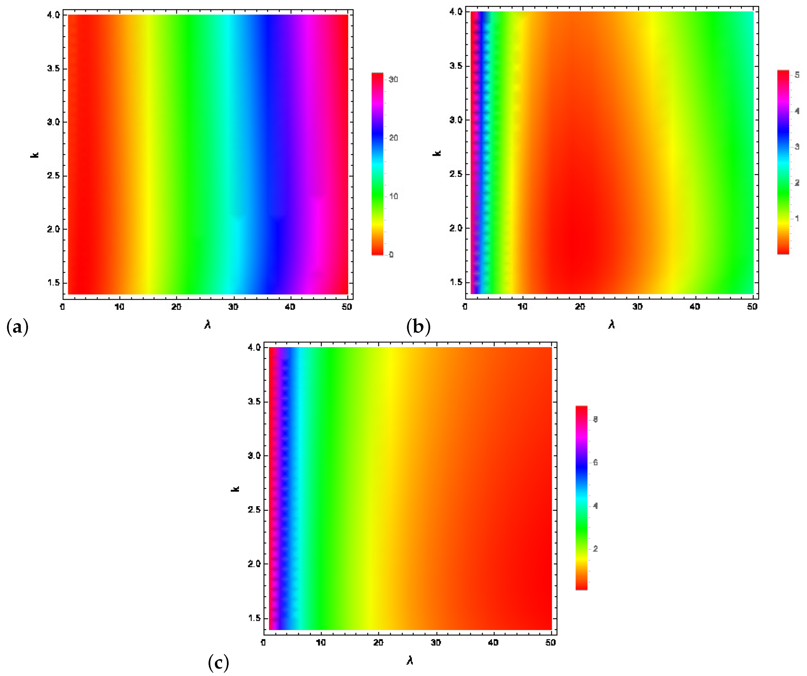
Equation (43) can be plotted as a surface in terms of the Weibull parameters $(k,\lambda )$. This means that for any $(k,\lambda )$, the corresponding point on the surface is $w_{min}$ that minimizes the relative entropy between the 1D-Weibull and Weibull distributions. Using a fixed value for $w_{min}$ as determined from (43), plots are shown for the relative entropy as a function of the Weibull parameters $(k,\lambda )$ in Figure 4. Figure 4a shows the relative entropy for $\lambda$ values between approximately zero to just over $\lambda =10$ where the divergence between the 1D-Weibull and Weibull distributions is zero or very close to zero. This occurs when $w_{min}=0.4$. In this region, see Figure 4a, and for the Weibull parameter values $(k,\lambda )$ shown, the Weibull distribution can be replaced by the 1D-Weibull. In order to have a relative entropy or divergence that is close to zero or even zero for values of $\lambda$ greater than say $\lambda =10$ requires using (43) to obtain $w_{min}=0.84$. The results are shown in Figure 4b where the relative entropy is close to zero or zero everywhere for approximately $10<\lambda <30$. Finally, small to zero divergence for higher values of the Weibull scale parameter, $30<\lambda \le 50$, can be achieved when $w_{min}=0.95$ as the results of Figure 4c show. Note that in all cases, the shape parameter values of interest for the Weibull distribution are covered, i.e., $k\in [1.4,4]$.

As further examination of the performance of the 1D-Weibull density, the Akaike information criterion A will be considered. The Akaike information criterion (AIC) has the following definition:

$$\begin{array}{c}\hfill A=2p-2log\left(L\left({\widehat{\theta }}_i\right)\right)+\frac{2p^2+2p}{n-p-1}\end{array}$$

(44)

where the idea is to use estimators for the parameters ${\theta }_i$ that maximise the log-likelihood function $L\left({\widehat{\theta }}_i\right)$. Here p represents the total number of parameters for each model being compared using certain data. The AIC penalises a model that has too many parameters because of over-fitting. This is especially true for small sample sizes n for which (44) is valid. When the sample size increases $n\to \infty$, the second term goes to zero and the AIC takes the form:

$$\begin{array}{c}\hfill A=2p-2log\left(L\left(\widehat{\theta }\right)\right)\end{array}$$

(45)

Another formulation of the AIC involves the residual sum of squares R, assuming that the residuals are distributed according to independent and identical normal distributions with zero mean,

$$\begin{array}{c}\hfill A=2p+nlog(R/n)\end{array}$$

(46)

In the case of the AIC involving the residual sum of squares, the idea is to have $R\to 0$. When this happens two models fit data equally well except that, according to the AIC, any discrepancy that might be present relies on the number of parameters p they each have. The same condition holds for the AIC formulated on the basis of the log-likelihood function, (45), however the log-likelihood function must be as large as possible before the first term dominates. Preference is for simpler models with fewer parameters that avoid the issues of over-fitting and complexity. On that basis, it appears that the 1D-Weibull with one less parameter compared to the Weibull has the advantage. The AIC value of the model that is generally smallest indicates the model that best fits the data. In order to compare the 1D-Weibull and Weibull using the AIC approach, care must be taken with the data being modelled. If the data is 1D-Weibull distributed it will fit better than the Weibull, see for example Figure 3. This is also because it has one parameter p less which means that the AIC values will be smaller. If the data is Weibull distributed, for cases where the 1D-Weibull has small or zero relative entropy with respect to the Weibull, both will fit the data equally well but with the better model being the 1D-Weibull since smaller AIC values will also be due to its one parameter compared to the two-parameter Weibull.

To better examine whether the 1D-Weibull has good performance relative to Weibull, random data was generated using the Frechet distribution as an alternative:

$$\begin{array}{c}\hfill {\rho }_F\left(x\right)=\frac{a}{s}{\left(\frac{x-m}{s}\right)}^{-(a+1)}{e}^{-{\left(\frac{x-m}{s}\right)}^{-a}}\end{array}$$

(47)

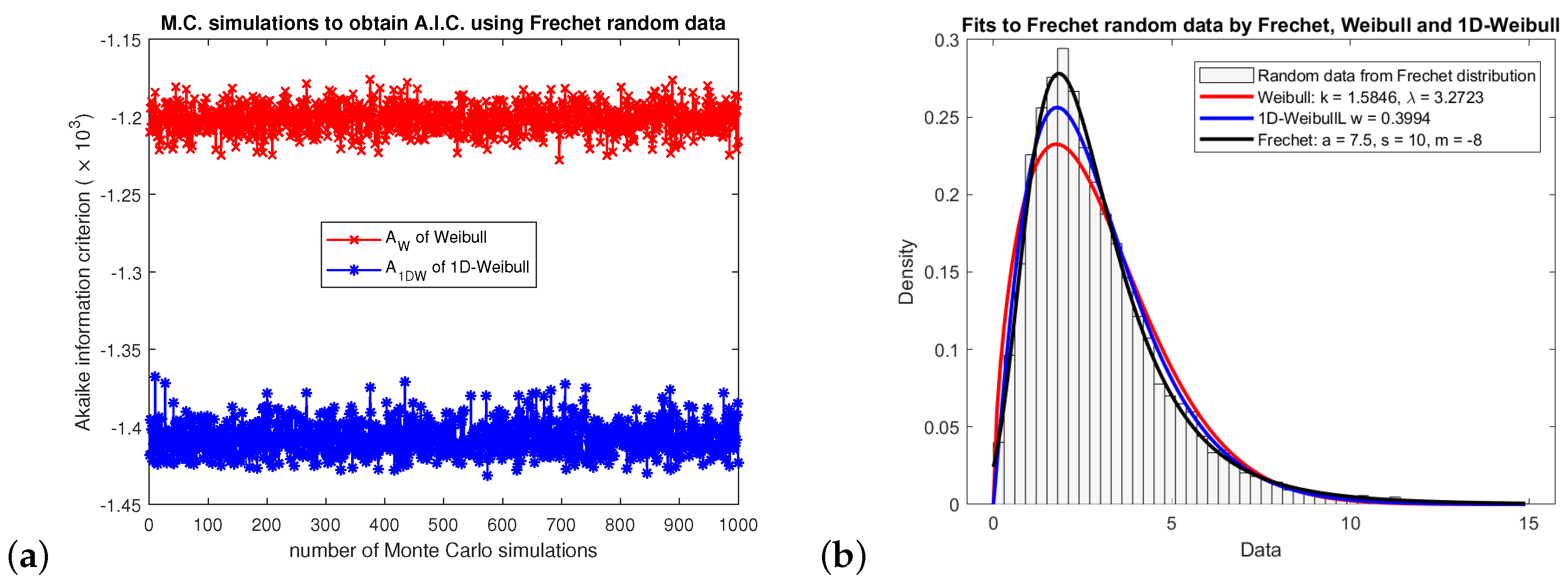
where the Frechet distribution has three parameters, a-shape, s-scale and m-location. Using seed values for the Frechet distribution, Frechet random variables were generated and ${10}^3$ Monte Carlo simulations were run with different random numbers generated each time. The 1D-Weibull and Weibull parameters were estimated each time and fitted to the Frechet density. The corresponding AIC values were calculated for each case. Figure 5a shows the Monte Carlo simulations and the AIC values. In all cases the 1D-Weibull has smaller values and hence it is the best model compared to Weibull for fitting the Frechet data. Figure 5b shows a typical fit to random Frechet data plotted as a density histogram together with fits from the 1D-Weibull, Weibull and the theoretical Frechet density.

So far, consideration has been given to finding a distribution, namely the 1D-Weibull, that has only one parameter and can fit data as well as the two-parameter Weibull when the relative entropy is small between them. It will be shown to fit data from different areas of research in Section 5. What will be considered next is a way of adding an extra parameter to standard one-parameter distributions. This modification not only allows the performance of the modified distribution to widen but it also maintains its previous one-parameter characteristics as a special limit of the second parameter. This will be done on the basis of transforms obtained from fractional mathematics that have been used to derive fractional distributions such as the Pareto [16,17]. The latter has been shown to model radar clutter extremely well. This idea is considered next and demonstrated by deriving a (fractional) two parameter version for the Exponential distribution.

4. A (Fractional) Two Parameter Exponential Distribution

The standard Exponential distribution has one parameter $\lambda \equiv 1/\mu$ where $\mu$ is the sample mean. In order to introduce another parameter to it that acts like the shape parameter of many two-parameter distributions it will be necessary to manipulate the variable x in the Exponential distribution,

$$\begin{array}{c}\hfill \rho \left(x\right)=\lambda e^{-\lambda x}\end{array}$$

(48)

The variable can be either continuous x or discrete $x_i$. The requirement is to find a simple transformation that relates x or $x_i$ to a modified version of themselves as a function of the second parameter $\alpha$. Once this new $x\left(\alpha \right)$ is obtained it is substituted into the CDF version of (48) to derive a two parameter form for the Exponential distribution. This will be done by using an operator that maps a function to a fractional or generalised version whose extra parameter $\alpha$ will act as the shape parameter. Let $f\left(y\right)=y$ be a i.i.d. random variable which will be transformed to the variable $x\left(\alpha \right)$ as follows:

$$\begin{array}{c}\hfill f\left(x\right)\mapsto {\int }_0^x\widehat{\Lambda }(x\mapsto y)f\left(y\right)dy\end{array}$$

(49)

where $\widehat{\Lambda }(x\mapsto y)$ is an operator that has the following form [18]:

$$\begin{array}{c}\hfill \widehat{\Lambda }(x\mapsto y)=\frac{1}{\Gamma (1-\alpha )}\frac{d}{dx}{\int }_0^{x}dy{(x-y)}^{-\alpha }\end{array}$$

(50)

The argument appearing in the operator $(x\mapsto y)$ means that the variable x maps on to the variable y as shown below. Let $f\left(x\right)=x$ be a variable that is to be modified by $f\left(y\right)=y$ to $x\left(\alpha \right)$. The integrand of (49) becomes:

$$\begin{array}{c}\hfill \widehat{\Lambda }(x\mapsto y)f\left(y\right)=\frac{1}{\Gamma (1-\alpha )}\frac{d}{dx}{\int }_0^{x}y{(x-y)}^{-\alpha }dy\end{array}$$

(51)

The integral can be carried out if a linear transformation $u=x-y$ is used. Then $dy=-du$ and substituting the transformation into the integrand gives

$$\begin{array}{cc}\hfill \widehat{\Lambda }(x\mapsto y)f\left(y\right)& =\frac{1}{\Gamma (1-\alpha )}\frac{d}{dx}{\int }_0^x\left(x{u}^{-\alpha }-u^{1-\alpha }\right)du\hfill \\ & =\frac{1}{\Gamma (1-\alpha )}\frac{d}{dx}\left[\frac{x{u}^{1-\alpha }}{1-\alpha }{|}_0^x-\frac{u^{2-\alpha }}{2-\alpha }{|}_0^x\right]\hfill \\ & =\frac{x^{1-\alpha }}{\Gamma (2-\alpha )}\hfill \end{array}$$

(52)

where the relation $\Gamma (2-\alpha )=(1-\alpha )\Gamma (1-\alpha )$ has been used. The final step is to map the variable x to y such that $\widehat{\Lambda }(x\mapsto y)f\left(y\right)$ becomes $\widehat{\Lambda }\left(y\right)f\left(y\right)$, that is,

$$\begin{array}{c}\hfill \widehat{\Lambda }\left(y\right)f\left(y\right)=\frac{y^{1-\alpha }}{\Gamma (2-\alpha )}\end{array}$$

(53)

Substituting into (49) and noting that $f\left(x\right)=x$ on the left means that this function (variable) is mapped as follows,

$$\begin{array}{c}\hfill x\mapsto \frac{1}{\Gamma (2-\alpha )}{\int }_0^x{y}^{1-\alpha }dy\end{array}$$

(54)

The integral is easy to calculate and using the fact that $\Gamma (3-\alpha )=(2-\alpha )\Gamma (2-\alpha )$, the final transformation for a variable x to its fractional analogue is,

$$\begin{array}{c}\hfill x\mapsto \frac{x^{2-\alpha }}{\Gamma (3-\alpha )}\end{array}$$

(55)

for the continuous case and

$$\begin{array}{c}\hfill \sum _i^n{x}_i\mapsto \frac{1}{\Gamma (3-\alpha )}\sum _i^n{x}_i^{2-\alpha }\end{array}$$

(56)

for the discrete case. It is now possible to use the continuous transformation to construct a fractional or two-parameter Exponential distribution. Replacing x in the standard CDF gives the following form

$$\begin{array}{c}\hfill \tilde{\rho }\left(x\right)=\left|1-exp\left(-\frac{\lambda }{\Gamma (3-\alpha )}{x}^{2-\alpha }\right)\right|\end{array}$$

(57)

The PDF is easily obtained using the derivative of the CDF:

$$\begin{array}{c}\hfill \rho \left(x\right)\equiv \left|\frac{d}{dx}\tilde{\rho }\left(x\right)\right|=\left|\frac{\lambda }{\Gamma (2-\alpha )}{x}^{1-\alpha }{e}^{-\frac{\lambda }{\Gamma (3-\alpha )}{x}^{2-\alpha }}\right|\end{array}$$

(58)

Notice that when $\alpha =1$ both the CDF and PDF collapse to the standard versions. Hence the fractional two-parameter Exponential also has the same performance characteristics as the standard Exponential in addition to its wider applicability due to the second parameter $\alpha$. The reason why the modulus is required is because the parameter $\alpha$ can also take any value that is real $(\alpha \in R)$ or complex $(\alpha \in C)$. This ensures that $\rho \left(x\right)\ge 0$ and avoids complex values. An important property that (58) must have if it is indeed a density is that it’s integral must be unity, otherwise it is not a probability density. It is easy to establish this since

$$\begin{array}{cc}\hfill \frac{\lambda }{\Gamma (2-\alpha )}{\int }_0^{\infty }{x}^{1-\alpha }{e}^{-\frac{\lambda }{\Gamma (3-\alpha )}{x}^{2-\alpha }}dx& =-e^{-\frac{\lambda }{\Gamma (3-\alpha )}{x}^{2-\alpha }}{|}_0^{\infty }\hfill \\ & =1\hfill \end{array}$$

(59)

and so the fractional or two-parameter Exponential distribution is a density. This means that the following properties hold:

$$\begin{array}{c}\hfill \underset{x\to 0}{lim}{\rho }_{exp}\left(x\right)=0;\underset{x\to \infty }{lim}{\rho }_{exp}\left(x\right)=0\end{array}$$

(60)

and

$$\begin{array}{c}\hfill \underset{x\to 0}{lim}{\tilde{\rho }}_{exp}\left(x\right)=0;\underset{x\to \infty }{lim}{\tilde{\rho }}_{exp}\left(x\right)=1\end{array}$$

(61)

The moments can be obtained via the usual process,

$$\begin{array}{c}\hfill <x^m>=\frac{\lambda }{\Gamma (2-\alpha )}{\int }_0^{\infty }{x}^{m+1-\alpha }{e}^{-\frac{\lambda }{\Gamma (3-\alpha )}{x}^{2-\alpha }}dx\end{array}$$

(62)

Using linear transformations and integration by parts it can be shown that the moments have the following closed form,

$$\begin{array}{c}\hfill <x^m>=\Gamma \left(1-\frac{m}{\alpha -2}\right){\left[\frac{\lambda }{\Gamma (3-\alpha )}\right]}^{\frac{m}{\alpha -2}}\end{array}$$

(63)

Setting $m=0$ in (63) gives the second axiom of probability which means the the moment is equal to unity over the entire integration domain. The expectation or mean is given by $m=1$:

$$\begin{array}{c}\hfill <x>=\Gamma \left(1-\frac{1}{\alpha -2}\right){\left[\frac{\lambda }{\Gamma (3-\alpha )}\right]}^{\frac{1}{\alpha -2}}\end{array}$$

(64)

When the parameter $\alpha$ takes on the value $\alpha =1$, the (fractional) two-parameter Exponential distribution collapses to the standard Exponential. Thus setting $\alpha =1$ into (64) gives the standard expectation:

$$\begin{array}{cc}\hfill <x>& =\Gamma \left(2\right){\left[\frac{\lambda }{\Gamma \left(2\right)}\right]}^{-1}\hfill \\ & =\frac{1}{\lambda }\hfill \\ & =\mu \hfill \end{array}$$

(65)

where $1/\lambda =\mu$ and $\mu$ is the standard expectation. Using $m=1$ and $m=2$, the variance $var(\alpha ,\lambda )=<x^2>-<x{>}^2$ becomes,

$$\begin{array}{c}\hfill var(\alpha ,\lambda )=\left[\Gamma \left(\frac{\alpha -4}{\alpha -2}\right)-{\Gamma }^2\left(\frac{\alpha -3}{\alpha -2}\right)\right]{\left[\frac{\lambda }{\Gamma \left(3-\alpha \right)}\right]}^{\frac{2}{\alpha -2}}\end{array}$$

(66)

The standard Exponential variance is obtained when $\alpha =1$ so that,

$$\begin{array}{cc}\hfill var\left(\lambda \right)& =\left[\Gamma \left(3\right)-{\Gamma }^2\left(2\right)\right]{\left[\frac{\lambda }{\Gamma \left(2\right)}\right]}^{-2}\hfill \\ & =\frac{1}{{\lambda }^2}\hfill \end{array}$$

(67)

as expected. Finally, to obtain the estimators for the two parameters $(\alpha ,\lambda )$ use of the maximum likelihood method is made where the likelihood function is:

$$\begin{array}{c}\hfill l(\alpha ,\lambda )=\frac{{\lambda }^n}{{\Gamma }^n(2-\alpha )}\prod _{i=1}^n{x}_i^{1-\alpha }{e}^{-\frac{\lambda x_i^{2-\alpha }}{\Gamma (3-\alpha )}}\end{array}$$

(68)

From this, the log-likelihood function is derived in the following form,

$$\begin{array}{c}\hfill L(\alpha ,\lambda )=nlog\left(\lambda \right)-nlog(\Gamma (2-\alpha ))+(1-\alpha )\sum _{i=1}^{n}log\left(x_i\right)-\frac{\lambda }{\Gamma (3-\alpha )}\sum _{i=1}^n{x}_i^{2-\alpha }\end{array}$$

(69)

Before deriving the estimator for $\widehat{\lambda }$ from (69), consider the alternative approach first. From (56) for a discrete variable, the fractional transform implies that the standard estimator $\widehat{\lambda }$ can be replaced as follows:

$$\begin{array}{c}\hfill \widehat{\lambda }={\left[\frac{1}{n}\sum _{i=1}^n{x}_i\right]}^{-1}\mapsto {\widehat{\lambda }}_{\alpha }={\left[\frac{1}{n\Gamma (3-\alpha )}\sum _{i=1}^n{x}_i^{2-\alpha }\right]}^{-1}\iff \sum _{i=1}^n{x}_i\mapsto \frac{1}{\Gamma (3-\alpha )}\sum _{i=1}^n{x}_i^{2-\alpha }\end{array}$$

(70)

When $\alpha =1$, ${\widehat{\lambda }}_{\alpha }=\widehat{\lambda }$. Returning to (69), the estimator for ${\lambda }_{\alpha }$ is given by,

$$\begin{array}{c}\hfill \frac{\partial L(\alpha ,\lambda )}{\partial \lambda }=0\mathrm{then}{\widehat{\lambda }}_{\alpha }={\left[\frac{1}{n\Gamma (3-\alpha )}\sum _{i=1}^n{x}_i^{2-\alpha }\right]}^{-1}\end{array}$$

(71)

which means that the fractional transform method for obtaining the estimator agrees with the maximum likelihood approach. If $\alpha$ is chosen to be any value $\alpha \in R$ or $\alpha \in C$ then the modulus is considered, i.e., $|{\widehat{\lambda }}_{\alpha }|$. The right-hand side of the $\lambda$’s is of course the sample (or population) mean $\mu$. Unfortunately, the estimator for the second (fractional) parameter $\alpha$ does not have a closed form and must be solved numerically similarly to how the shape parameter for the standard Weibull k is obtained. From (69), the requirement is to solve for

$$\begin{array}{c}\hfill \frac{\partial L(\alpha ,\lambda )}{\partial \alpha }=0\end{array}$$

(72)

Then the estimator $\widehat{\alpha }$ is obtained numerically from:

$$\begin{array}{c}\hfill \frac{{\psi }^{\left(1\right)}(2-\widehat{\alpha })}{{\psi }^{\left(0\right)}(2-\widehat{\alpha })}=\frac{1}{n}\sum _{i=1}^{n}log\left(x_i\right)+\frac{\lambda }{\Gamma (3-\widehat{\alpha })}\left[\frac{1}{n}{\psi }^{\left(0\right)}(3-\widehat{\alpha })\sum _{i=1}^n{x}_i^{2-\widehat{\alpha }}-\frac{1}{n}\sum _{i=1}^{n}log\left(x_i\right)x_i^{2-\widehat{\alpha }}\right]\end{array}$$

(73)

where ${\psi }^{\left(0\right)}(·)$ and ${\psi }^{\left(1\right)}(·)$ are the poly-gamma functions of order zero and one respectively. Using (71), $\lambda$ can be eliminated in (73).

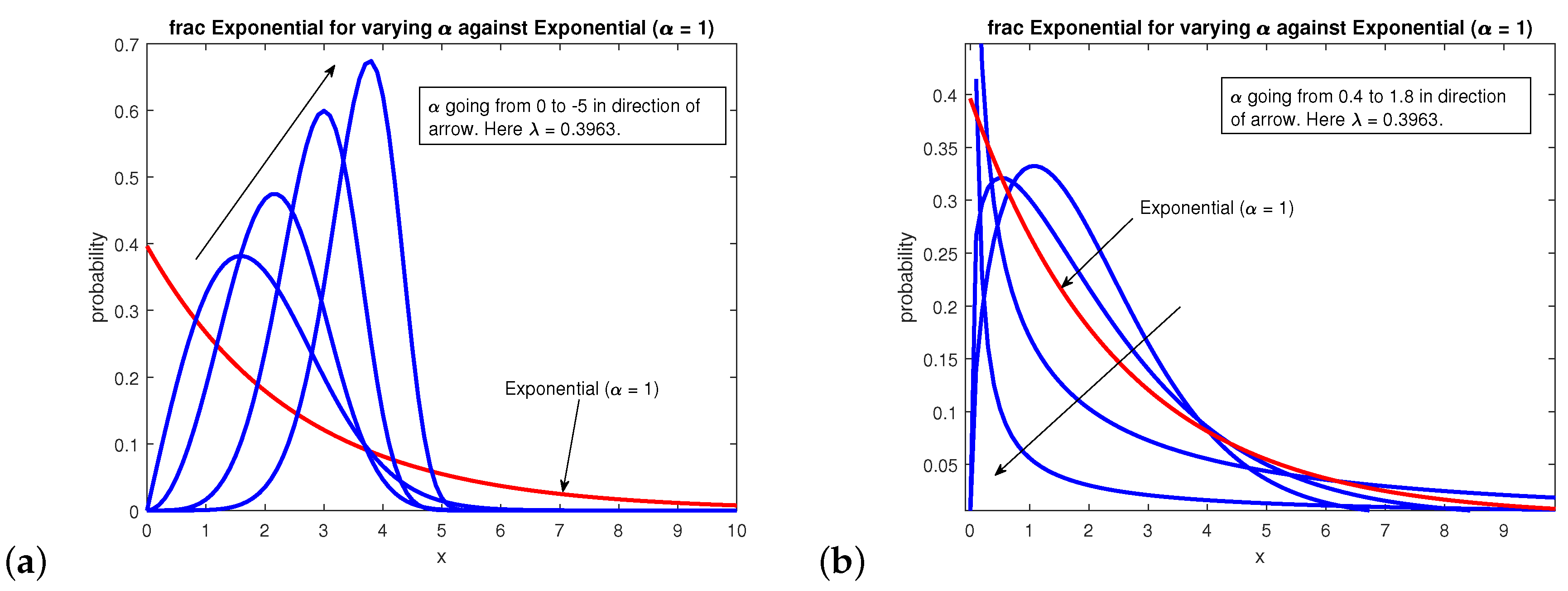
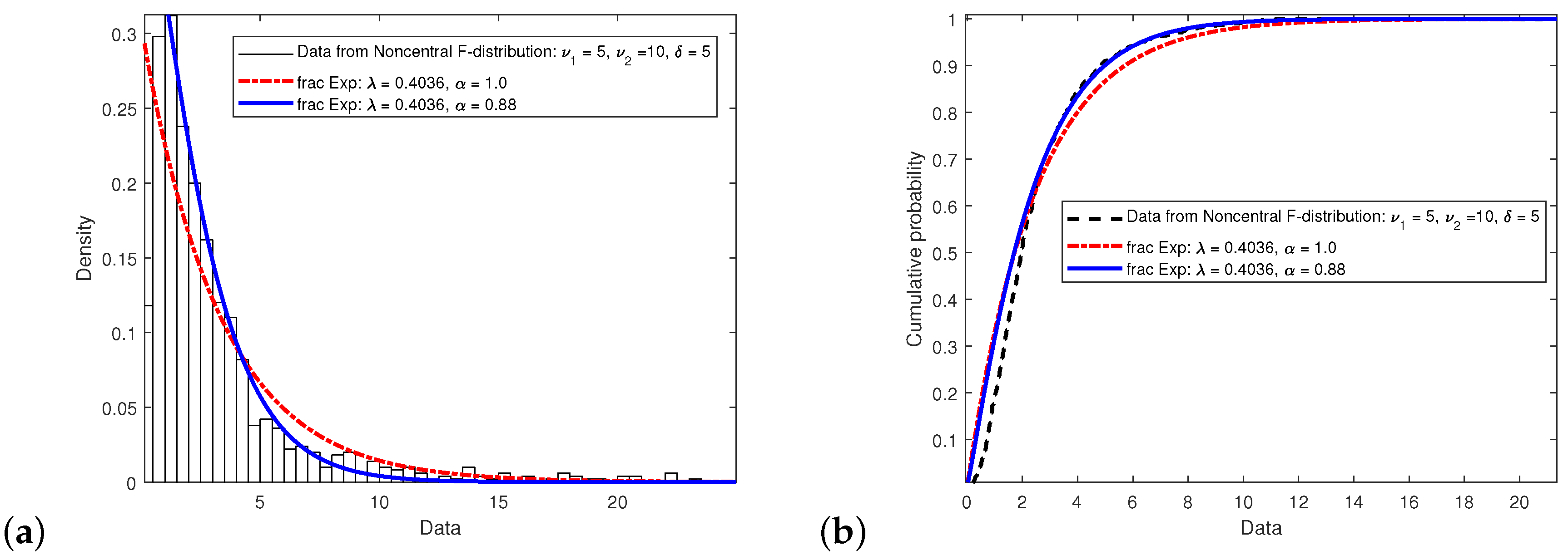
Figure 6 shows plots for different values of $\alpha$ including negative ones. Again this is possible since $\alpha \in C$ and $\alpha \in R$. The conventional Exponential density is a special case when $\alpha =1$, see (58) in the limit $\alpha =1$. Furthermore, the fractional exponential displays mathematical characteristics that are Weibull in nature as well as those of extreme value-type distributions. The standard Exponential and the two-parameter Exponential distributions were tested against random data generated by the non-local F-distribution which has three parameters: two that are the degree of freedom ${\nu }_1$ and ${\nu }_2$ respectively and the locality parameter $\delta$. When $\delta =0$, the non-local F-distribution reduces to the F-distribution. The reason why data was chosen from this distribution is because the Exponential with only one parameter $\lambda$ is not expected to fit the three parameter F-data well as Figure 7 shows. Nevertheless by modifying the Exponential distribution to a two parameter form, it is possible to achieve better fits to the data by varying $\alpha$ while keeping $\lambda$ fixed. 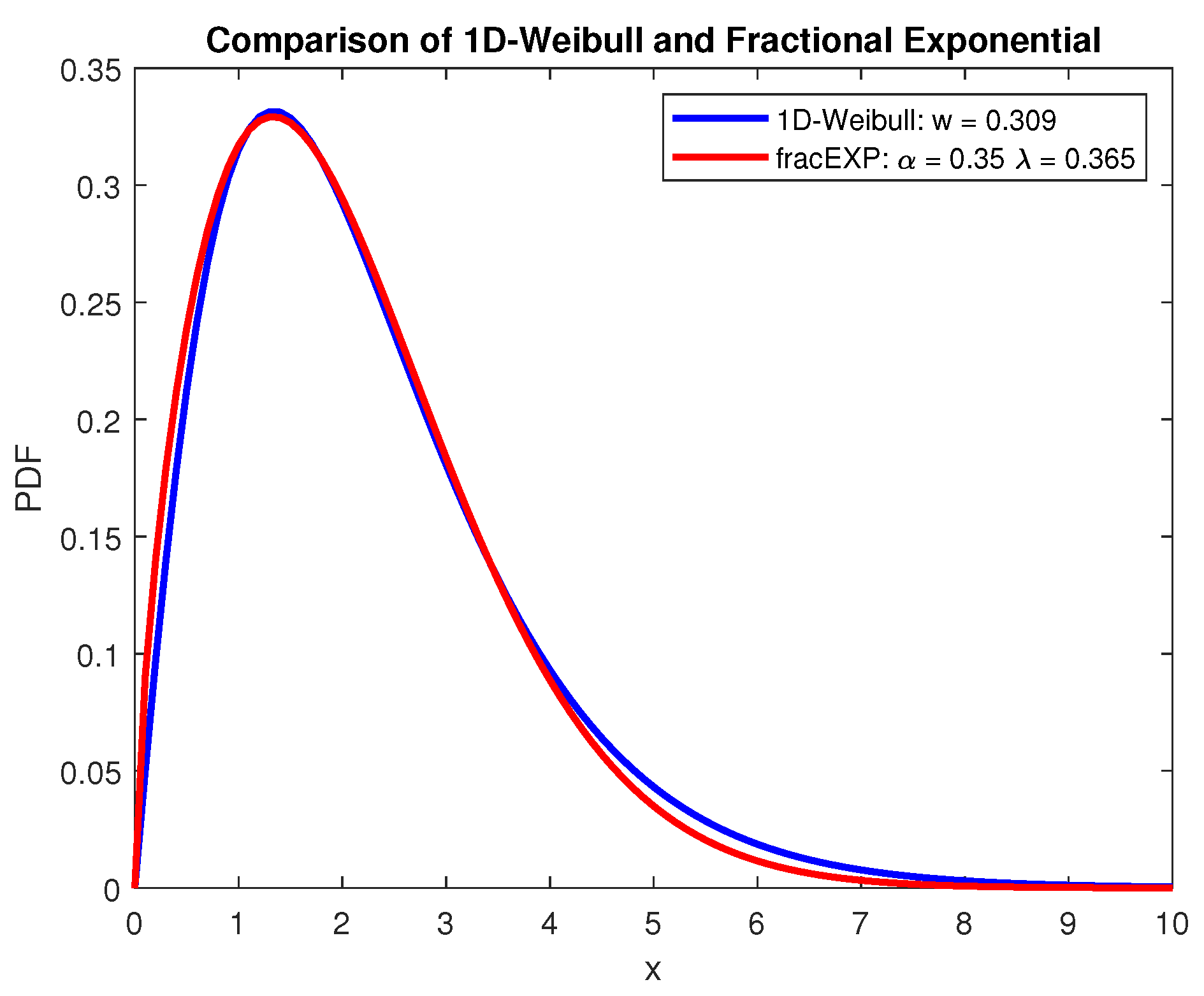As a further comparison, Figure 8 shows the 1D-Weibull and (fractional) two-parameter Exponential densities using non-optimised parameters. What is interesting is that in essence both of these distributions should not have Weibull-type characteristics. This is because the 1D-Weibull has only one parameter while the Exponential has a decaying trend. By modifying the Exponential to two parameters, it not only has the standard Exponential decay characteristics but it also exhibits Weibull and extreme value behaviour too.

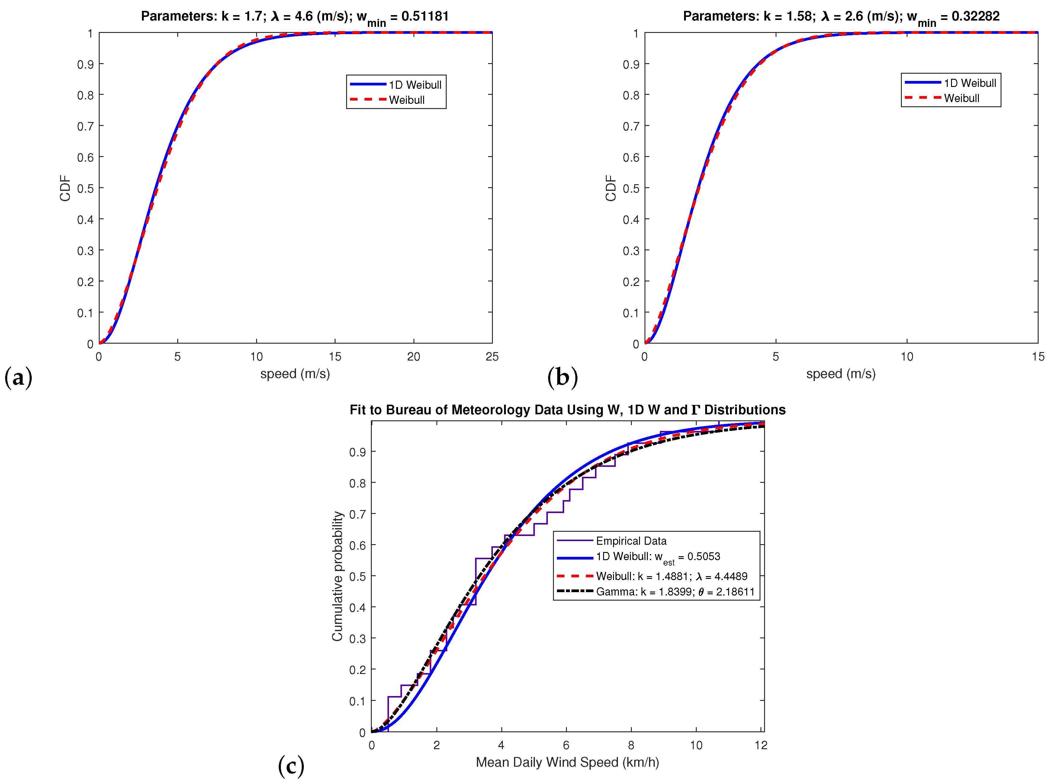
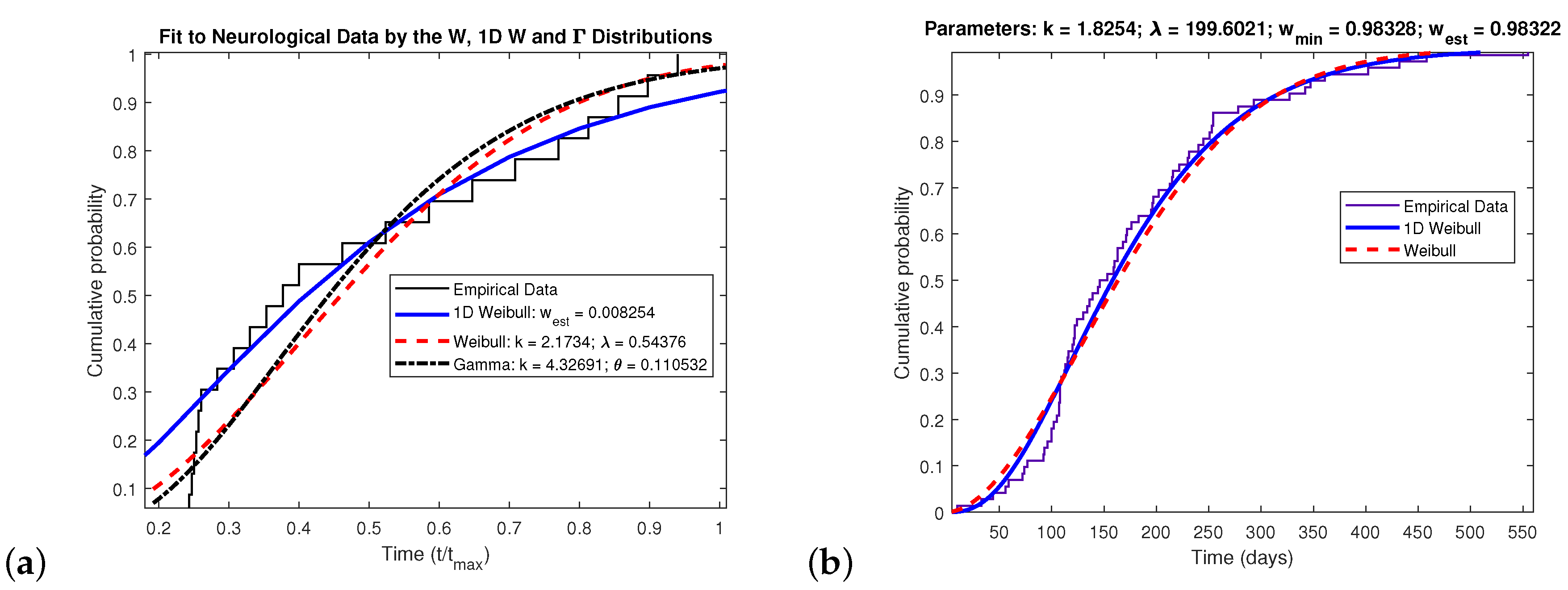
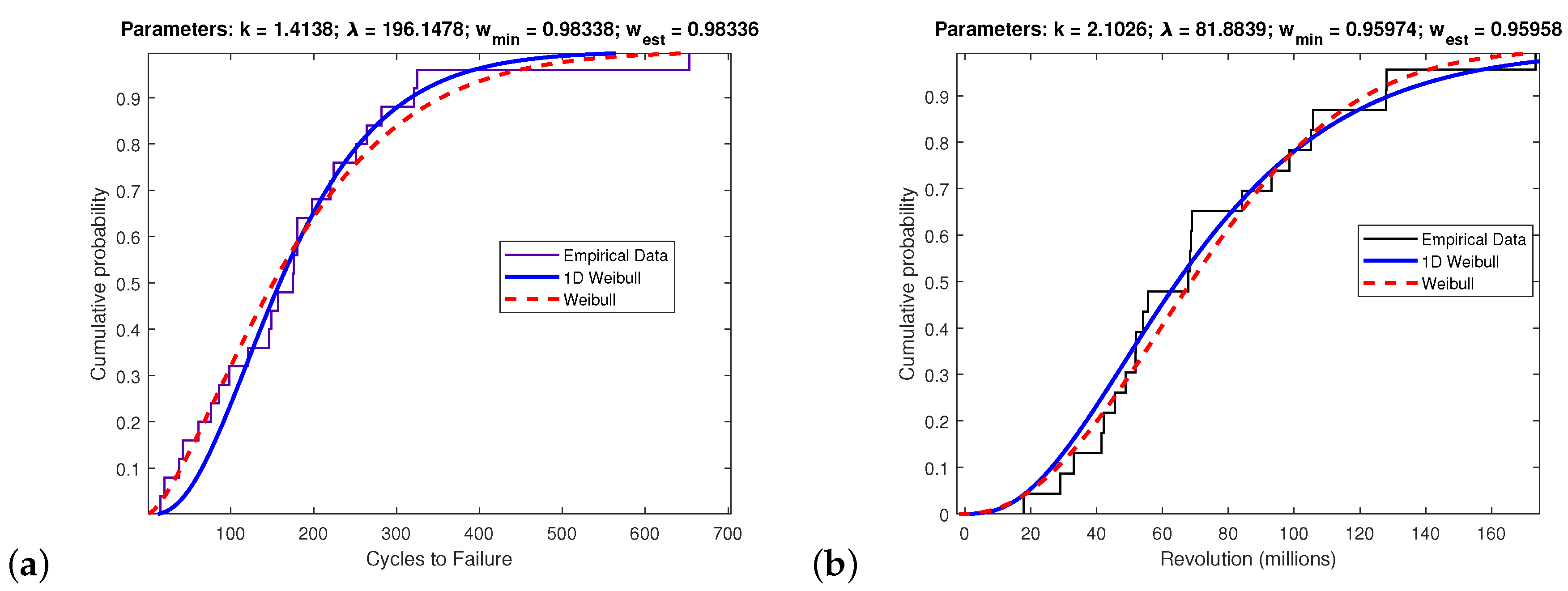
It should be clear from previously that the divergence between the 1D-Weibull and conventional Weibull indicates for what Weibull parameters $(k,\lambda )$ the 1D-Weibull matches the performance of the Weibull. In other words, regardless of the data being investigated, if the Weibull fits such data then it is also possible to ascertain whether the 1D-Weibull does too. Whenever the divergence is zero or small enough, it is then possible to replace the two-parameter Weibull with the one-parameter 1D-Weibull which only requires the sample mean to fit such data. In order to examine the performance of the 1D-Weibull, real data will be tested in this Section taken from different fields of research.

5. Application of the 1D-Weibull to Real Data

5.1. Meteorological Data

The study of the speed profile of wind is very important for energy conversion using wind-turbines for example. In such studies it is necessary to characterise the wind speed distribution at a particular site and typically this is accomplished using the Weibull distribution. The performance of the 1D-Weibull and conventional Weibull is compared on wind energy data as discussed in [19]. The authors show that the best distribution for modelling wind speed data is in fact the Weibull distribution and proceed to estimate the parameters, namely the shape k and scale $\lambda$, that best fit the data using a number of methods. The part density energy method (PDEM) is shown to estimate the Weibull parameters more accurately than the other methods. For this reason the PDEM results are used to compare the performance of the 1D-Weibull and Weibull. Figure 9a shows results for wind data obtained from location 17 out of the entire 29 locations studied in the paper [19]. The parameter $w_{min}$ is obtained from (43) for the Weibull parameters given, i.e., ($k=$ 1.7, $\lambda =$ 4.6). Later when results are compared with the empirical CDF of other data, it will be shown that in all cases $w_{min}\approx \widehat{w}$, where $\widehat{w}\equiv w_{est}$ is given by the estimator (16). In other words, the maximum likelihood estimator for the 1D-Weibull (which depends only on the mean) is essentially equal to the value of w that minimizes the divergence between the 1D-Weibull and Weibull distributions as discussed previously.

In the paper by Lorenz [20], data collected on Martian wind speeds was analysed from the Viking 1 and 2 landers. It was shown that the Weibull distribution is very accurate in describing the variation of wind on the surface of Mars. Figure 9b shows the performance of the 1D-Weibull and Weibull for data collected by the Viking 1 lander during the first 0–100 sols. Similar analysis has also been done to other data collected at different sol periods to confirm typical performance as shown in Figure 9b but have been excluded for brevity reasons. The results of Figure 9a,b confirm the divergence relation between the 1D-Weibull and Weibull because for the $(k,\lambda )$ parameters in the figures that describe real wind speed data, the convergence between the 1D-Weibull and Weibull is zero or very close to zero as Figure 4a shows. Using data obtained from the Australian Bureau of Meteorology (BoM) [21], Figure 9c shows fits to the mean daily wind speed in km/h by the 1D-Weibull and Weibull distributions. As a comparison, the Gamma-distribution is also shown with corresponding estimated parameters from the data set. Given that the data is the mean daily wind speed, the fitted data is susceptible to outliers which have a dramatic effect on the fits of all the distributions.

5.2. Hydrological Data

In [22], data was analysed which was concerned with the rate of water consumption during summer. For further details, the reader can refer to the paper [22]. Figure 10 shows the fit to the summer data by the 1D-Weibull and Weibull distributions. Even though the 1D-Weibull is a one parameter distribution, it performs really well compared to the two-parameter Weibull. Observe that for the 1D-Weibull, both the estimated w from the data and the predicted version from the Weibull parameters (43), are approximately equal as discussed previously.

5.3. Medical and Viral Data

Data taken from [23] consists of experiments done to study memory retention as a function of time in seconds. The data has also been analysed and discussed in [24]. Figure 11a shows a fit to this data set by the 1D-Weibull and Weibull distributions. In addition, the Gamma-distribution, with corresponding parameters, is also included as a comparison. The 1D-Weibull fits this data better than both the standard Weibull and Gamma distributions respectively. In [25,26], data has been presented that concerns the survival time in days of 72 guinea pigs that have been infected by the tubercle bacilli virus. The 1D-Weibull and Weibull have been fitted to this data as Figure 11b shows. Notice once again that the maximum likelihood estimator $\widehat{w}\equiv w_{est}$ is approximately equal to the theoretically predicted version $w_{min}$ which utilises the Weibull shape and scale parameters.

5.4. Industrial Data

Modelling processes that have a given lifetime is a subject area of great interest in many areas of science and engineering. This is especially true in the manufacturing industry where products are tested rigorously to ascertain how many cycles or time is required before they fail. Two such data sets are fitted here using the 1D-Weibull and Weibull distributions [26,27]. In the first data set, twenty five 100 cm specimens of yarn are tested at a given strain level. The data considers the number of cycles before failure (breakage). Figure 12a shows the empirical CDF against the 1D-Weibull and Weibull distributions. The other data set [26,27] investigates the endurance of deep groove ball bearings. Lifetime tests are conducted for twenty three ball bearings and the number of revolutions (in millions) before failure is represented in the data set. This data is fitted by the 1D-Weibull and Weibull distributions and is shown in Figure 12b. Once again, in both Figure 12a,b, the predicted and estimated values of the parameter w are approximately equal in each case.

6. Conclusions

A new one-parameter 1D-Weibull distribution was presented that can replace the two-parameter conventional Weibull for a large set of values of the latter’s parameters, i.e., it is a very good approximation to the Weibull distribution with validity beyond certain unique or trivial cases. This was verified by examining the relative entropy between them. The 1D-Weibull has excellent performance on real data from various areas when compared to the Weibull and gamma distributions and only requires the estimation of one parameter that only depends on the sample mean as opposed to the Weibull and Gamma that require the estimation of two parameters. It also avoids the need to compute parameters using transcendental numerical means as is required for the Weibull shape parameter k. An alternative approach was also considered by using fractional mathematics to derive a (fractional) two-parameter Exponential distribution that collapses to the standard version as a limit. This distribution approximates Weibull too but also exhibits its own interesting characteristics including those of extreme value distributions. The 1D-Weibull was a reduction in the number of parameters to one while the two-parameter Exponential was an increase of parameters from one to two.

This opens up the possibility of creating new or ‘approximate’ distributions to other established versions that have a smaller (or larger) number of parameters but with comparable performance in the solution of many scientific, mathematical and engineering problems.