Article

Unveiling Wildfire Dynamics: A Bayesian County-Specific Analysis in California

1
Department of Mathematics, Clarkson University, Potsdam, NY 13699, USA
2
Department of Computer Science, Clarkson University, Potsdam, NY 13699, USA
3
Department of Computer Science, University of Saskatchewan, Saskatoon, SK S7N 5A2, Canada
*
Author to whom correspondence should be addressed.
J 2024, 7(3), 319-333; https://doi.org/10.3390/j7030018
Submission received: 2 June 2024 / Revised: 13 August 2024 / Accepted: 16 August 2024 / Published: 19 August 2024

Abstract

:
Recently, the United States has experienced, on average, costs of USD 20 billion due to natural and climate disasters, such as hurricanes and wildfires. In this study, we focus on wildfires, which have occurred more frequently in the past few years. This paper examines how various factors, such as the PM10 levels, elevation, precipitation, SOX, population, and temperature, can influence the intensity of wildfires differently across counties in California. More specifically, we use Bayesian analysis to classify all counties of California into two groups: those with more wildfires and those with fewer wildfires. The Bayesian model incorporates prior knowledge and uncertainty for a more robust understanding of how these environmental factors impact wildfires differently among county groups. The findings show a similar effect of the SOX, population, and temperature, while the PM10, elevation, and precipitation have different implications for wildfires across various groups.

1. Introduction

In the past three years, natural disasters have resulted in USD 20 billion of damage in the United States. This amount is significantly higher compared to the USD 6.7 and USD 12.8 billion incurred in the two decades of the 2000s and 2010s, respectively [1]. In the United States, many states, such as Florida, South Carolina, and California, have experienced natural disasters such as hurricanes, wildfires, storms, and floods. Climate and natural disasters endanger the lives of animals and humans both directly and indirectly and raise concerns for communities, ecosystems, and public health [2,3]. These disasters also impose financial burdens on individuals; for example, the average cost of evacuations in 2020 per family was USD 5000 [4]. Therefore, due to the financial and health burdens imposed by these disasters on societies, it is important to better understand the impact of the related factors on wildfires [5,6,7,8,9,10,11,12,13,14,15].
Recent research has focused extensively on understanding the factors that influence the occurrence and intensity of natural disasters, particularly wildfires, in the United States. The studies by Kolden et al. [13] and Joseph et al. [14] utilize Bayesian models to assess fire risks in California, to understand the significant roles of infrastructure, climate factors, and the housing density in wildfires’ ignition and spread. They suggest that future urban expansion in fire-prone areas could exacerbate the fire risks and that the likelihood of extreme wildfires is closely tied to the dryness and temperature. The work of Li et al. [15] highlights a shift in wildfire patterns over the last two decades and notes a substantial increase in small human-caused fires, which has altered the distribution of burned areas across the state.
Keeley and Syphard [16] compare historical and recent large wildfires in California and consider the increasing frequency and destruction of such events driven by extreme weather conditions. Their findings suggest that the growing population and expansion of infrastructure in highly flammable areas have amplified the damage caused by wildfires in recent years. These insights emphasize the need for empirical models that can assess the current and future fire risks based on a combination of environmental factors and human activities, to help us to better understand and compare the dynamics driving wildfires’ occurrence and intensity.
The National Integrated Drought Information System mentions that, from 1971 to 2021, human-caused climate change contributed to a +172% increase in burned areas, with a +320% increase from 1996 to 2021 [17]. The National Park Service reports that humans cause about 85 percent of all wildfires yearly in the United States. The California Department of Forestry and Fire Protection states that fires have resulted in at least 85 civilian deaths, injured 12 civilians and five firefighters, and spread across an area of 153,336 acres [18]. An article in USA Today [19] reports more frequent and devastating fires occurring in California. These disasters can be due to the varying climatic characteristics and different types of landscape in California, such as the Mediterranean climate along the coast, desert climate in southeastern regions, steppe climate in interior valleys, and highland climate in mountainous areas. Moreover, California encompasses a wide range of ecosystems, from highly populated urban areas to less populated rural areas with diverse natural environments. These diverse ecological features make it difficult to understand and control the factors that cause natural disasters [6,16,20,21,22,23,24,25].
In this study, we aim to better understand the wildfire dynamics in California counties by analyzing and comparing the effects of environmental and ecological factors, such as the particulate matter (PM10) level, elevation, precipitation, sulfur oxides (SOX), population density, and temperature [26,27,28,29,30]. Each of these factors and the complex interactions formed by their relationships may increase the likelihood of the occurrence of wildfires. Therefore, we utilize statistical analysis [31,32] to investigate the complex relationships of the different factors among all 58 counties in California. It is worth noting that the aim of this work is not to predict wildfires or investigate the most important aforementioned factors causing wildfires, but rather to utilize Bayesian statistical models to compare these factors among different counties in California. The county level was chosen for the study because of the availability of data and the opportunity to compare different counties, rather than looking at the entire state of California as a large area.
The structure of this paper is as follows. In Section 2, we provide details of the data creation process and perform initial investigations on the data. In Section 3, we discuss the Bayesian analysis of variance, Bayesian regression, and software and programming packages used in this study. In Section 4, we present the results of the Bayesian analysis and simulations of wildfires in California. In Section 5, we discuss the results more broadly and compare the impacts of the variables on different states. Finally, in Section 6, we draw conclusions and offer insights for future research.

2. Exploratory Data Analysis

2.1. CAL FIRE Dataset

Various datasets are available for fires in California. We use the California Open Data-CAL FIRE dataset [33], available on their website. This contains variables such as the name of the fire, the date of occurrence, the event that created it, the time that it was extinguished, and the last update. In terms of location, the dataset contains county-level aggregated data with the exact location of the fire, the total wildfire density for the fire, and the identified longitude and latitude at the beginning of the fire. The dataset ranges from 2013 to 2023 and contains all fires that occurred during this period.

2.2. NOAA Data

We use data from the National Oceanic and Atmospheric Administration (NOAA) to include the temperature and precipitation [34]. The NOAA dataset contains the aggregated maximum, minimum, and average temperatures and precipitation at the monthly level for each county. The NOAA keeps historic records of numerous climate-related variables, which are also available through their website.

2.3. ARB Emissions Data

We also consider the California Air Resources Board (ARB) for data on emissions [35]. The ARB provides county-level data based on air quality standards for six common criteria pollutants set by the US Environmental Protection Agency [36]. The dataset includes annual summaries of pollutant levels measured across various monitoring stations in each county, which are then used to evaluate compliance with national air quality standards. These data can be used to understand the relationship between air pollution and wildfire activity, as pollutants like PM10 and SOX can both influence and be influenced by fire incidents. Additionally, the ARB emissions data allow for the analysis of trends over time to identify any correlations between changes in pollutant levels and the frequency or intensity of wildfires.

2.4. CSAC Population Data

Finally, we use the California State Association of Counties (CSAC) for data on county areas and populations [37]. This dataset helps us to calculate population statistics and the wildfire density. The CSAC provides detailed information on the population size, density, and growth rates for each county, as well as geographic and administrative boundaries. These population metrics are used to assess the human impact on wildfire occurrences. This dataset also supports the analysis of the ways in which demographic factors, including changes in land use and housing density, correlate with the spatial and temporal patterns of wildfires across the state.

2.5. Analysis of Average Acres Burned

Using the data described above, we combine fires of all sizes in each year. Figure 1 shows the average acres burned from 2013 to 2023. A large number of fires occurred in 2018, 2020, and 2021. This was caused by three record-breaking fires that were so large that they increased the average dramatically in each of these years. The 2018 Mendocino Complex fire, which burned through counties including Colusa, Lake, Mendocino, and Glenn, was the most expansive fire in California’s history. These fires have burned approximately 460,000 acres of land [18]. In 2020, the August Complex fire burned a final total of 1,032,648 acres, resulting in the largest fire burned in California. In 2021, the Dixie fire burnt even more land mass than the August Complex fire, and 400 more structures were damaged. Some fires are devastating and span larger areas and cover multiple counties or even states, such as the complex fires of 2020 and 2021.
Table 1 provides a comprehensive overview of the following factors: wildfire density (per acre), average altitude (meters), average temperature (degrees Fahrenheit), average precipitation (millimeters), population density (population per acre), PM10 (micrograms per cubic meter), and SOX (parts per million). The average values provide a measure of the central tendency and the standard deviation quantifies the dispersion or variability of each factor. For instance, the wildfire density has a mean of 0.688; that is, on average, there are 0.688 wildfires per acre, with a standard deviation of 1.236. The wide range of wildfire densities, from 0.01 to 8.71, indicates large variation across counties. We also observe a wide discrepancy in variables such as the elevation, population, PM10, and SOX. The elevation ranges from 30 to 2216 m, the temperature ranges from 77.3 °F to 109.87 °F, precipitation ranges from 2.5 to 33 mm, PM10 ranges from 1.259 to 284 μ g/m3, and, finally, SOX ranges from 0.004 to 13.7 ppb. As described in the previous section, such variations arise from California’s topographical features.
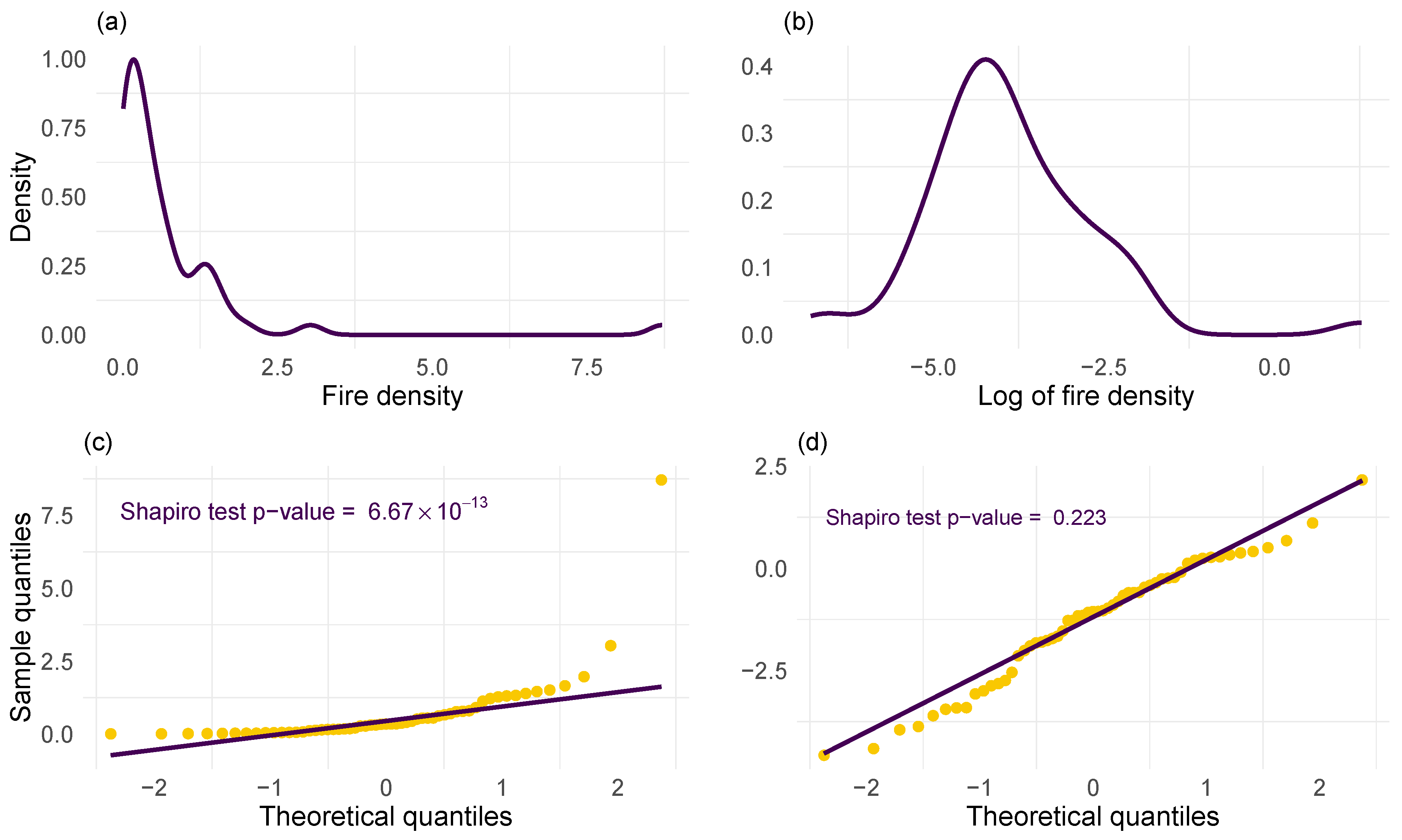
Because our main focus in this work is centered around the wildfire density, we take a closer look at this variable. Figure 2a illustrates the distribution of the wildfire density. This distribution is heavily right-skewed and does not follow a normal distribution. This non-normality is not unusual in real-world datasets but adversely affects the accuracy of many statistical models [38,39]. We apply a log transformation to the observed wildfire density to reduce the skewness, resulting in a distribution that appears more symmetric, as shown in Figure 2b. While visual diagnosis can provide a general idea about the distribution, a more robust and rigorous test should be performed to analyze the normality. We utilize the Shapiro test [40]. As shown in Figure 2c, the qq plot does not follow the theoretical normal distribution and the p-value = 6.67 × 10 13 associated with the Shapiro test verifies the non-normality of the observed wildfire density. However, Figure 2d and the p-value = 0.223 verify the normality of the log-transformed wildfire density.
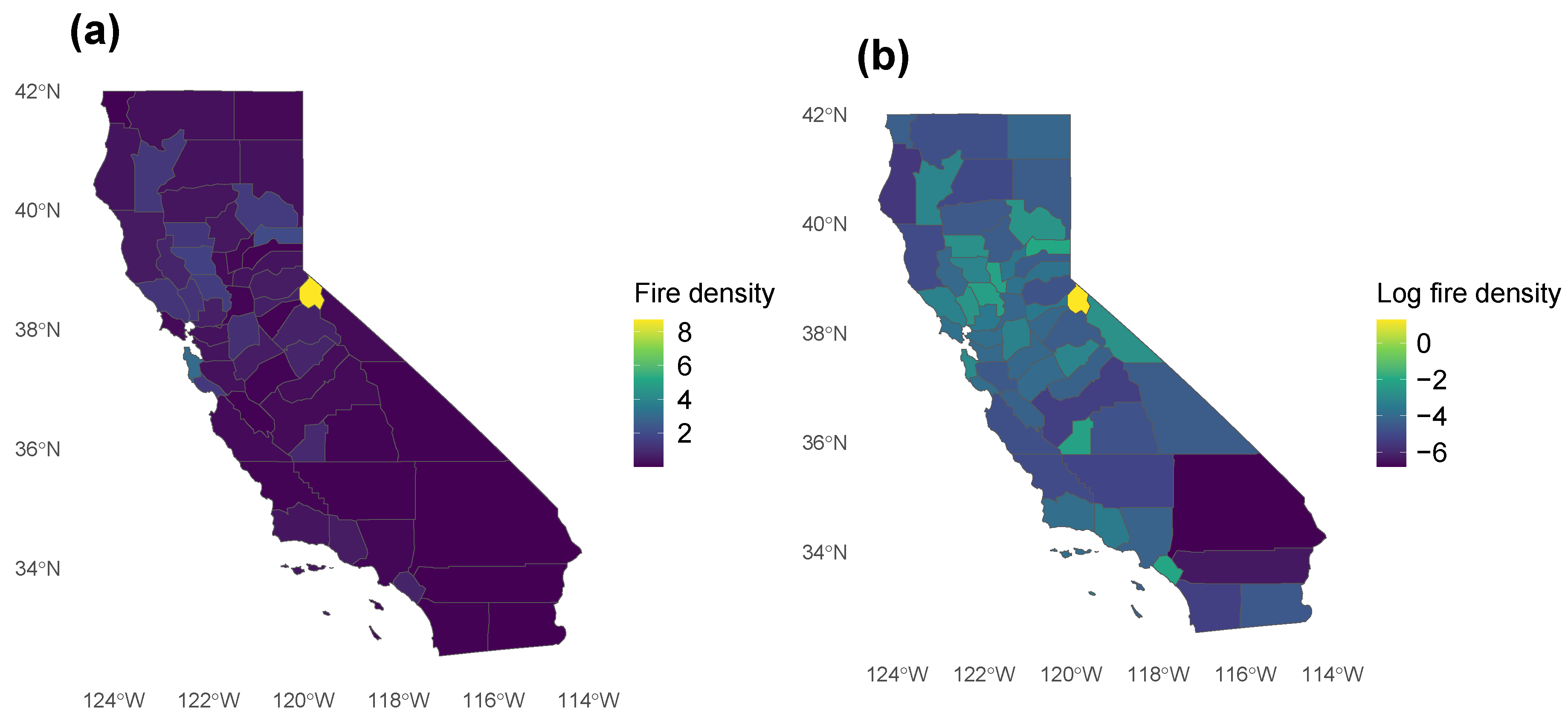
On the other hand, the transformed data align better with the characteristics of wildfire data in that extreme values may be more accurately represented on a logarithmic scale [41]. This is illustrated in Figure 3 across counties. Figure 3a shows that Alpine County (shown in yellow) has an extreme fire density compared to other counties and consequently dominates them. Figure 3b illustrates the log transformation of the mean wildfires. Log transformation mitigates the impact of extreme values and enables a more accurate comparison.

3. Methodology

3.1. Analysis of Variance

Analysis of variance (ANOVA) is a widely used statistical method for the determination of whether there are any statistically significant differences between the means of three or more groups. In general, ANOVA is characterized by two components: (i) between-group variability, which quantifies the extent to which the means of different groups vary from the global mean, and (ii) within-group variability, which quantifies variations within each group [38]. ANOVA simultaneously compares the means of different groups without isolating each group and discarding the effect of the groups on each other. More flexible models, such as Bayesian ANOVA, perform better for complex data structures involving many interacting factors. Bayesian ANOVA can take the prior knowledge of the variables, as well as uncertainty in the model, into account. Bayesian analysis provides a posterior analysis, such as examining credible intervals and probabilistic statements about differences between groups [31,32,42]. The Bayesian ANOVA methodology is discussed below.
Suppose that there are m groups. For each group j { 1 , 2 , , m } , let Y i j denote the ith observation within the jth group. Then, the Bayesian ANOVA of Y i j is modeled as
Y i j | μ j , σ y N ( μ j , σ y 2 ) μ j | μ , σ μ i n d N ( μ , σ μ 2 ) μ N ( m , s 2 ) σ y Exp ( l y ) σ μ Exp ( l μ ) ,
where μ j models how the factors vary within group j, μ represents the prior model of the global mean, and σ y and σ μ represent the prior variability in the means within and between groups, respectively. This model considers two sources of variability, the variability inside each group and also the variability among the groups, i.e., Var ( Y i j ) = σ y 2 + σ μ 2 . The σ y and σ μ parameters are chosen to reflect our beliefs about the typical magnitude of the variability in the individual observations and county means. More information can be found in Johnson et al. [31] and Gelman et al. [32].
In this study, the hierarchical Bayesian ANOVA structure allows us to consider the variability of the wildfires inside each individual county, along with the variability of the wildfires among all counties.

3.2. Bayesian Regression

Similar to classical linear regression methods [38], Bayesian regression models a response variable as a linear combination of different variables. Bayesian regression considers the uncertainty and variability in the model parameters and provides a probability distribution for these parameters. This is the advantage of Bayesian models compared to classical linear regression, which is built upon the assumption of fixed parameters. In addition, Bayesian regression is very flexible, can produce predictions and estimations for more complex data, and is more robust for smaller sample sizes of data.
Suppose that Y denotes the response variable and ( X 1 , X 2 , , X p ) is a set of p variables. The Bayesian regression model is defined as follows [31].
Data : Y i | β 0 , β 1 , β 2 , , β 7 , σ N μ i , σ 2 μ i = β 0 + β 1 X i 1 + β 1 X i p Priors : β 0 N m 0 , s 0 2 β 1 N m 1 , s 1 2 β 2 N m 2 , s 2 2 β p N m p , s p 2 σ Exp ( l ) ,
where β 0 , β 1 , , β p represent the prior coefficients of the linear regression model, and σ is the standard deviation of the error term representing the variability of the response variable that is not explained by the variables ( X 1 , X 2 , , X p ) . The priors N ( m 0 , s 0 2 ) , N ( m 1 , s 1 2 ) , …, N ( m 7 , s p 2 ) are normal distributions based on our prior beliefs about the values of the regression coefficients. The prior Exp ( l ) for σ represents a prior belief in non-negative values for the standard deviation. These priors and the likelihood function together form the Bayesian regression model. Considering these priors, we updated our beliefs based on the observed data to estimate the posterior.
Initiating priors is the first step in Bayesian analysis. Priors form a bridge between what we already knew and what we can see in the data. Priors affect the prediction and estimation results; therefore, it is important to carefully consider them. When we have sufficient information to estimate our priors, we use this information and knowledge to define the prior model, which is known as informative priors. Specifying informative priors could be challenging when analyzing complex data, and they may impose some bias on the model and obscure the true variations in the data. In such situations, weakly informative priors can be used to allow the observed data to guide the formation of prior distributions. Once the prior distributions are established, the model uses the data to update the priors to produce posterior distributions. Posterior distributions are used to estimate or predict response variables. More detailed information about Bayesian regression, priors, posteriors, and other Bayesian concepts can be found in Johnson et al. [31] and Gelman et al. [32].

3.3. Software

The statistical software R version 4.1.2 was used to analyze the data and utilize the methods, along with the following main libraries in our coding: rstan, rstanarm, tidybayes, bayesplot, tidyverse, tidycensus, and bayesrules. The rstan package is an interface to the Stan programming language for Bayesian analysis. rstanarm is an extension of rstan and provides a more user-friendly environment for Bayesian regression models. tidybayes is a tidy data principle in Bayesian analysis. bayesplot provides an extensive library of plotting functions. tidyverse includes a collection of important data science packages for data manipulation and visualization. tidycensus is used to access and analyze US Census data in a tidy format. Every aspect of the results presented in this paper can be perfectly replicated from a clean and unobfuscated R script, which we provide in the Supplementary Information.

4. Results

4.1. Bayesian ANOVA Results

Due to the heterogeneous nature of the geographical and environmental landscape of California, we first analyze how the wildfire density differs across counties. We first use Bayesian ANOVA to provide statistical evidence of the variability in the wildfire density among the counties. We then use the insights gained from this initial analysis to classify the counties with the highest and lowest wildfire densities. The findings from the Bayesian ANOVA model for the comparison of the wildfire density among all 58 counties in California are displayed in Figure 4. The x-axis and y-axis show the names of the counties and the log of the wildfire density, respectively. The plot contains 80% posterior credible intervals for each county. The longer the vertical bar, the greater the variability and uncertainty in calculating the averages.
We use the rstanarm R package to produce 10,000 iterations for each Markov chain for each parameter. The first 5000 iterations are considered a “warm-up” sample, and the second 5000 are kept as the final Markov chain sample [43]. Table 2 summarizes the posterior summary of the Bayesian ANOVA model and shows how the wildfire density varies across counties. The average value of the wildfire density in the entire state is estimated to be −4.05. The 80% credible interval ranges from −4.23 to −3.86 and quantifies the uncertainty of the mean estimation. The model also verifies the variability of 0.993 between states. This variability emphasizes the diverse influence of county-specific factors on fire densities and contributes to the overall complexity of the model. The average variation within states is estimated to be 2.11, which captures the unexplained variability within counties.
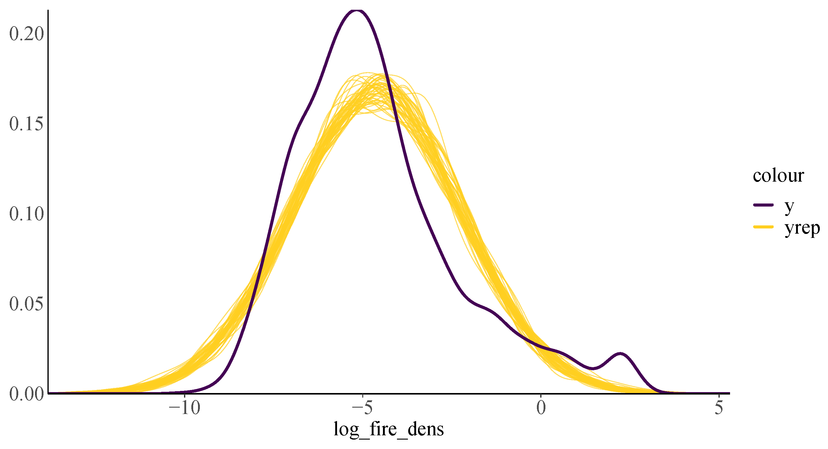
To assess how well our ANOVA model replicates the observed data, we performed a posterior predictive check. Figure 5 confirms that the model is not biased and can produce predictions (yellow curves) with characteristics similar to the observed wildfire density data (dark purple curve). The capacity of the model to capture the key characteristics and intrinsic variability (such as spread and central tendency) in the data is demonstrated by the relative consistency between the posterior predictive values and the data.
As discussed in Figure 4, Table 2 verifies the variation in the wildfire density between the counties. In addition, a posterior predictive check confirmed that the Bayesian ANOVA model could capture the variability of the data. Therefore, we use the discrepancies among different counties to classify them into two groups based on their mean differences for a more in-depth analysis. More specifically, the counties with the highest average wildfire density are considered as “top” counties, and the counties with the lowest average wildfire density are considered as “bottom” counties. We now consider these two groups to compare the variables within each group. This will help us to better understand the differences in the wildfire density between the two county groups.

4.2. Bayesian Regression Results

As discussed, the Bayesian ANOVA showed heterogeneity in the wildfire density. Following this analysis, we now focus on comparing the factors contributing to the variability in the wildfire density between the top and bottom counties. We use Bayesian regression to compare the relationships between the wildfire density and other factors among the top and bottom groups, to understand the factors that contribute to the observed differences. Specifying informative priors for the analysis of wildfires could be challenging because the dynamics of wildfire occurrence can change and are not fully predictable. We choose weakly informative priors to be broad enough to allow a range of plausible values for the parameters.
We use the rstanarm R package to perform Bayesian regression with four chains, each chain with 10,000 iterations. Table 3 and Table 4 present the summary statistics of the model parameters resulting from the Bayesian regression. These tables provide information, such as the estimated values for each factor, their uncertainties and credible intervals, the effective sample size (Neff Ratio), and the Gelman–Rubin statistic (Rhat), for both the top and bottom counties. For example, for the top counties, a one-unit increase in temperature (in Fahrenheit, log scale) is associated with an average change of 0.0133 in the wildfire density per acre according to the model. However, instead of focusing on interpreting each individual number, our goal is to emphasize the comparison of each factor between the top and bottom counties to identify key differences and trends. Before performing this comparison, we must check to ensure that the model converges effectively and that the results are reliable. One criterion is the Neff ratio, which quantifies the number of independent samples that must be considered to produce an accurate posterior approximation. Any Neff ratio greater than 0.1 can be considered acceptable [43]. The other criterion is Rhat, which compares the variability across all chains combined with the variability within any individual chain in the Monte Carlo Markov Chain (MCMC) simulation. A value less than 1.05 is considered acceptable [43]. Both the Neff Ratio and Rhat for all variables are within the suggested acceptable region, which indicates a reliable estimation process and confirms the convergence across the four Markov chains.
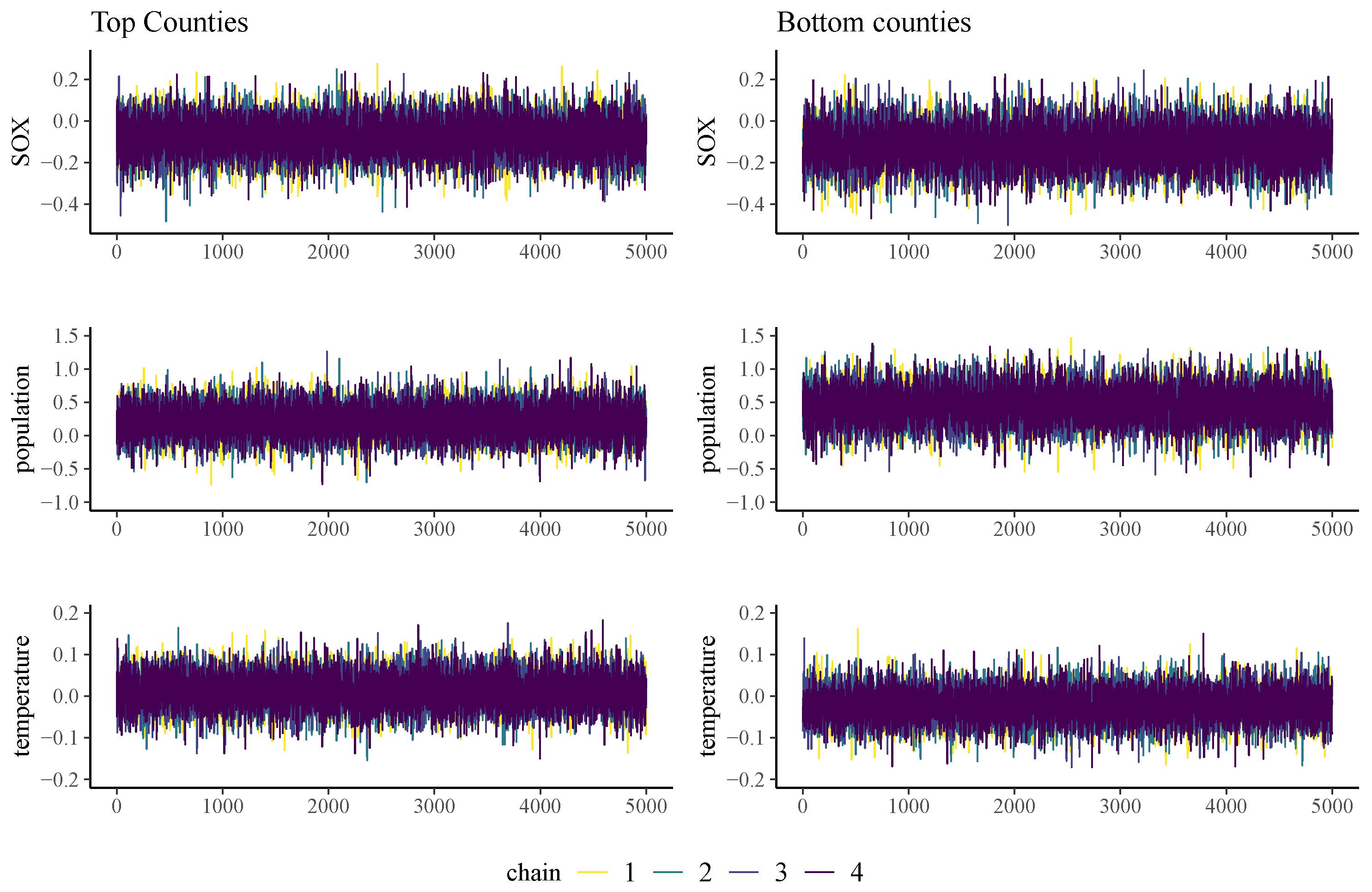
Figure 6 and Figure 7 show the MCMC trace plots for the factors to compare the different factors among the top and bottom counties. Based on the distinct patterns in the trace plots, we can identify and compare the influences of the predictors among the top and bottom counties (discussed in Section 5). These plots can also be used as diagnostic tools to ensure the convergence of the MCMC chains to a stationary distribution and for effective parameter space exploration. All trace plots demonstrate consistent and reasonable behavior and mix quickly for both county groups. This proves the stability of our Bayesian regression model and shows that the algorithm effectively navigates the parameter space and provides robust estimates for the considered predictors.
The consistent overlapping of the chains with no discernible trends or patterns for each plot in Figure 6 and Figure 7 indicates that the chains are well mixed and have converged to a stationary distribution. This behavior is important in ensuring that the posterior distributions derived from these chains are representative of the true underlying model. While the visual inspection of these trace plots is essential, it should be noted that convergence and mixing are also supported by the quantitative diagnostics shown in Table 3 and Table 4. The combination of visual and quantitative assessments ensures that the Bayesian regression model provides robust and reliable estimates for the factors influencing the wildfire dynamics in both the top and bottom counties. Therefore, the Bayesian regression model effectively captures the relationships between the predictors and provides stable estimates. More information regarding mixing and convergence can be found in Johnson et al. [31] and Gelman et al. [32].

5. Discussion

In Section 4, we found similar impacts of the SOX, population, and temperature on wildfires in both the top and bottom counties. We should emphasize that the same impact of these three factors on wildfires does not necessarily mean that there is no relationship or causation between the factors and wildfires. It has been found that (i) SOX is associated with industrial activities, affects air quality, and can increase the risk of wildfires; (ii) the population density is associated with human habitation patterns and results in human-related ignition sources; and (iii) a high temperature enhances the combustibility of vegetation and results in more extremely hot days. Therefore, while there are associations between these factors and wildfires, we do not observe any significant difference in their impact on wildfires between the top and bottom counties. This could be due to the presence of other, stronger underlying factors or the indirect effects of these factors on the two groups. For example, higher SOX emissions trap heat and indirectly increase the wildfire risk in some counties. Recent studies have showed that high levels of pollutants like SOX correlate with increased fire incidents in regions with high industrial activity and and a larger human presence increases the ignition sources [26,27,28,44,45,46], and our findings show that this correlation is similar among the county groups.
We found a different impact of PM10 on wildfires in the top counties compared to the bottom counties. The association between PM10 and wildfires has been previously investigated and demonstrated [47,48]. However, this discrepancy among the top and bottom counties is important and could be due to the complex relationship between fires and PM10 and their causality—does a fire cause an increase in PM10, or does PM10 lead to more fire incidents? This inconsistency warrants further investigation to understand the underlying mechanisms and potentially identify additional factors that contribute to this variation between counties.
The next disparity between the top and bottom counties is the effect of elevation factors on wildfires. Since our focus was more on the comparison between the top and bottom counties than the actual values, we found that the effect of elevation on wildfires was three times larger in the top counties than in the bottom counties. The significant impact of elevation on wildfires shows that higher altitudes often experience distinct ecological conditions that can either mitigate or exacerbate fires’ spread [49]. This emphasizes the importance of considering topographical factors in wildfire risk assessments. The heightened impact of elevation on the top counties could be attributed to the combined effect of terrain-related factors on fire dynamics. Elevated regions often exhibit different vegetation types, moisture levels, and ecological patterns that can influence wildfires [50,51]. Moreover, high elevation may change the land use patterns, human activities, and vegetation composition and exert a more dominant influence on wildfire occurrence.
The third disparity between the top and bottom counties was precipitation. The “absolute” effect of precipitation was nine times larger in the top counties, which emphasizes the clear impact of precipitation on wildfires. In the top counties, the negative relationship between precipitation and wildfires suggested an intuitive dynamic: precipitation is positively related to moisture, which prevents fires from starting and expanding. When lush vegetation becomes dry, it could provide a fuel for wildfires [30,52]. This finding is consistent with the broader literature, which highlights the dual role of precipitation in both preventing and, paradoxically, promoting wildfires when excessive moisture leads to more biomass growth that later dries out [53].

6. Conclusions and Future Work

In this study, we analyzed wildfires in California from a different and new perspective to compare the different variables that impact wildfires across counties. First, we classified all counties into top and bottom county groups based on the wildfire density in each county. California has a diverse topography, climate patterns, and human activities, which contribute to its unique and varied regional characteristics. Therefore, we closely examined how the factors functioned differently in the top and bottom counties by utilizing the inherent variability across California’s diverse regions. We found that the SOX, population, and temperature universally influence wildfires in both top and bottom counties, while the PM10, elevation, and precipitation have different effects on wildfires in the top and bottom counties.
The population and temperature similarly influence wildfires across both top and bottom counties because they are pervasive factors that collectively contribute to the essential conditions that are needed for wildfire occurrence. Regardless of whether a county experiences frequent or infrequent wildfires, these factors interact to create an environment where wildfires can ignite and spread. The different impacts of PM10, elevation, and precipitation among the top and bottom counties are due to the localized (such as [16]) nature of these factors. In contrast to the temperature and population, which have a more similar influence across regions, PM10, elevation, and precipitation are more sensitive to the local conditions. These factors interact with the specific environmental, industrial, and geographical characteristics of each county, which leads to differing impacts on the wildfire risk among the top and bottom county groups.
Taking these similarities and differences into account can help us to explore further and gain a deeper understanding of why some factors influence wildfires consistently across counties, whereas others have a differentiated impact. By employing time-series Bayesian regression analysis, we can expand our comprehension and achieve more precise outcomes. This would allow us to identify trends and patterns in the timing of wildfires and the changing effects of the variables over time. Furthermore, adding spatial information about wildfires (e.g., the precise longitude and latitude of fire incidents) could enrich the model. More complex data require a more advanced and computationally feasible model. We recommend utilizing convolutional neural network (CNN) models to process multilayer fire images of counties for more in-depth insights.

Supplementary Materials

The following supporting information can be downloaded at: https://www.mdpi.com/article/10.3390/j7030018/s1.

Author Contributions

Data curation, S.P., A.L. (Alex Lindquist), N.S., V.Y.; Writing—original draft, S.P., A.L. (Alex Lindquist), N.S., V.Y.; Writing—review and editing, A.L. (Ali Lotfi), J.G., M.M.; Formal analysis, S.P., A.L. (Alex Lindquist), N.S., V.Y.; Supervision, A.L. (Ali Lotfi), J.G., M.M. All authors have read and agreed to the published version of the manuscript.

Funding

This research received no external funding.

Institutional Review Board Statement

Not applicable.

Informed Consent Statement

As the study did not involve humans, the informed consent statement is not applicable.

Data Availability Statement

The data are available in the Supplementary Materials.

Acknowledgments

The authors thank the reviewers whose feedback improved the clarity of the manuscript.

Conflicts of Interest

The authors declare no conflicts of interest.

References

  1. Gusner, P. Natural Disaster Facts And Statistics 2023. Forbes Advis. Available online: https://www.forbes.com/advisor/homeowners-insurance/natural-disaster-statistics/#:~:text=Jefferson%20Parish%2C%20Louisiana.-,How%20Many%20Natural%20Disasters%20Occur%20Each%20Year%3F,dollar%20climate%20disasters%20per%20year (accessed on 13 August 2024).
  2. Oliver-Smith, A. Climate change, disasters, and development in Florida. In Disasters in Paradise: Natural Hazards, Social Vulnerability, and Development Decisions; Rowman & Littlefield: Lanham, MD, USA, 2019; Volume 203. [Google Scholar]
  3. Bell, J.E.; Herring, S.C.; Jantarasami, L.; Adrianopoli, C.; Benedict, K.; Conlon, K.; Escobar, V.; Hess, J.; Luvall, J.; Garcia-Pando, C.P.; et al. Ch. 4: Impacts of Extreme Events on Human Health. In The Impacts of Climate Change on Human Health in the United States: A Scientific Assessment. III; Technical Report; US Global Change Research Program: Washington, DC, USA, 2016. [Google Scholar]
  4. Group, C. Mandatory Natural Disaster Evacuations Prove Costly for Homeowners. 2020. Available online: https://www.crcgroup.com/Tools-Intel/post/Mandatory-Natural-Disaster-Evacuations-Prove-Costly-for-Homeowners (accessed on 12 May 2024).
  5. National Academies of Sciences, Engineering, and Medicine. Implications of the California Wildfires for Health, Communities, and Preparedness: Proceedings of a Workshop; National Academies Press: Washington, DC, USA, 2020. [Google Scholar]
  6. Calkin, D.; Short, K.; Traci, M. California wildfires. In US Emergency Management in the 21st Century; Routledge: Oxfordshire, UK, 2019; pp. 155–182. [Google Scholar]
  7. Domínguez, D.; Yeh, C. Social justice disaster relief, counseling, and advocacy: The case of the Northern California wildfires. Couns. Psychol. Q. 2020, 33, 287–311. [Google Scholar] [CrossRef]
  8. MacDonald, G.; Wall, T.; Enquist, C.A.; LeRoy, S.R.; Bradford, J.B.; Breshears, D.D.; Brown, T.; Cayan, D.; Dong, C.; Falk, D.A.; et al. Drivers of California’s changing wildfires: A state-of-the-knowledge synthesis. Int. J. Wildland Fire 2023, 32, 1039–1058. [Google Scholar] [CrossRef]
  9. Moser, S.C.; Ekstrom, J.; Franco, G. Our Changing Climate 2012: Vulnerability & Adaptation to the Increasing Risks from Climate Change in California; University of California: Berkeley, CA, USA, 1 July 2012. [Google Scholar]
  10. Schweizer, D. Fine Particulate Matter and Wildland Fire Smoke: Integrating Air Quality, Fire Management, and Policy in the California Sierra Nevada. Ph.D. Thesis, UC Merced, Merced, CA, USA, 2016. [Google Scholar]
  11. Goldman, T. Consequences of Sprawl: Threats to California’s Natural Environment and Human Health; University of California Press: Berkeley, CA, USA, 2001. [Google Scholar]
  12. Pathak, T.B.; Maskey, M.L.; Dahlberg, J.A.; Kearns, F.; Bali, K.M.; Zaccaria, D. Climate change trends and impacts on California agriculture: A detailed review. Agronomy 2018, 8, 25. [Google Scholar] [CrossRef]
  13. Kolden, C.A.; Weigel, T.J. Fire risk in San Diego County, California: A weighted Bayesian model approach. Calif. Geogr. Soc. 2007, 47, 42–60. [Google Scholar]
  14. Joseph, M.B.; Rossi, M.W.; Mietkiewicz, N.P.; Mahood, A.L.; Cattau, M.E.; St. Denis, L.A.; Nagy, R.C.; Iglesias, V.; Abatzoglou, J.T.; Balch, J.K. Spatiotemporal prediction of wildfire size extremes with Bayesian finite sample maxima. Ecol. Appl. Online Libr. 2019, 29, e01898. [Google Scholar] [CrossRef] [PubMed]
  15. Li, S.; Banerjee, T. Spatial and temporal pattern of wildfires in California from 2000 to 2019. Sci. Rep. 2021, 11, 8779. [Google Scholar] [CrossRef]
  16. Keeley, J.E.; Syphard, A.D. Large California wildfires: 2020 fires in historical context. Fire Ecol. 2021, 17, 1–11. [Google Scholar] [CrossRef]
  17. Nidis, N. Study Finds Climate Change to Blame for Record-Breaking California Wildfires; National Integrated Drought Information System: Boulder, Co, USA, 2023. [Google Scholar]
  18. Fire, C. Current Emergency Incidents Dataset; State of California, California Department of Forestry and Fore Protection: Sacramento, CA, USA, 2023. [Google Scholar]
  19. Petras, G.; Thorson, M.; Sullivan, S. Why California wildfires have increased in frequency and size. 2018. Available online: https://www.usatoday.com/pages/interactives/news/california-wildfires-carr-fire-data/ (accessed on 12 May 2024).
  20. Mooney, H.; Zavaleta, E. Ecosystems of California; University of California Press: Berkeley, CA, USA, 2016. [Google Scholar]
  21. Li, S.; Dao, V.; Kumar, M.; Nguyen, P.; Banerjee, T. Mapping the wildland-urban interface in California using remote sensing data. Sci. Rep. 2022, 12, 5789. [Google Scholar] [CrossRef]
  22. Huntsinger, L.; Barry, S. Grazing in California’s Mediterranean Multi-Firescapes. Front. Sustain. Food Syst. 2021, 5, 715366. [Google Scholar] [CrossRef]
  23. Garfin, G.; Jardine, A.; Merideth, R.; Black, M.; LeRoy, S. Assessment of Climate Change in the Southwest United States: A Report Prepared for the National Climate Assessment; Island Press: Washington, CA, USA, 2013. [Google Scholar]
  24. Goss, M.; Swain, D.L.; Abatzoglou, J.T.; Sarhadi, A.; Kolden, C.A.; Williams, A.P.; Diffenbaugh, N.S. Climate change is increasing the likelihood of extreme autumn wildfire conditions across California. Environ. Res. Lett. 2020, 15, 094016. [Google Scholar] [CrossRef]
  25. Minnich, R.A. California fire climate. In Fire in California’s Ecosystems; University of California Press: Berkeley, CA, USA, 2018; pp. 11–25. [Google Scholar]
  26. Viswanathan, S.; Eria, L.; Diunugala, N.; Johnson, J.; McClean, C. An analysis of effects of San Diego wildfire on ambient air quality. J. Air Waste Manag. Assoc. 2006, 56, 56–67. [Google Scholar] [CrossRef] [PubMed]
  27. Naqvi, H.R.; Mutreja, G.; Shakeel, A.; Singh, K.; Abbas, K.; Naqvi, D.F.; Chaudhary, A.A.; Siddiqui, M.A.; Gautam, A.S.; Gautam, S.; et al. Wildfire-induced pollution and its short-term impact on COVID-19 cases and mortality in California. Gondwana Res. 2023, 114, 30–39. [Google Scholar] [CrossRef] [PubMed]
  28. Fasullo, J.T.; Phillips, A.; Deser, C. Evaluation of leading modes of climate variability in the CMIP archives. J. Clim. 2020, 33, 5527–5545. [Google Scholar] [CrossRef]
  29. Huang, Y.; Wu, S.; Kaplan, J.O. Sensitivity of global wildfire occurrences to various factors in the context of global change. Atmos. Environ. 2015, 121, 86–92. [Google Scholar] [CrossRef]
  30. Fasullo, J.; Otto-Bliesner, B.; Stevenson, S. ENSO’s changing influence on temperature, precipitation, and wildfire in a warming climate. Geophys. Res. Lett. 2018, 45, 9216–9225. [Google Scholar] [CrossRef]
  31. Johnson, A.A.; Ott, M.Q.; Dogucu, M. Bayes Rules!: An Introduction to Applied Bayesian Modeling; CRC Press: Boca Raton, FL, USA, 2022. [Google Scholar]
  32. Gelman, A.; Carlin, J.B.; Stern, H.S.; Rubin, D.B. Bayesian Data Analysis; Chapman and Hall/CRC: Boca Raton, FL, USA, 1995. [Google Scholar]
  33. CAGOV. California Open Data. 2023. Available online: https://data.ca.gov/dataset/cal-fire (accessed on 12 May 2024).
  34. NOAA. Climate Data Online, National Centers for Environmental Information; National Oceanic and Atmospheric Administration: Washington, DC, USA, 2023.
  35. ARB. Current California GHG Emission Inventory Data; California Air Resources Board: Riverside, CA, USA, 2023. [Google Scholar]
  36. EPA. Greenhouse Gas Reporting Program (GHGRP); United States Environmental Protection Agency: Washington, DC, USA, 2023.
  37. CSAC. Population Estimates for Counties and Cities–1970 to 2018 Dataset; California State Association of Counties: Sacramento, CA, USA, 2023. [Google Scholar]
  38. Faraway, J.J. Linear Models with R; Chapman and Hall/CRC: Riverside, CA, USA, 2004. [Google Scholar]
  39. Dobson, A.J.; Barnett, A.G. An Introduction to Generalized Linear Models; Chapman and Hall/CRC: Boca Raton, FL, USA, 2018. [Google Scholar]
  40. Shapiro, S.S.; Wilk, M.B. An analysis of variance test for normality (complete samples). Biometrika 1965, 52, 591–611. [Google Scholar] [CrossRef]
  41. Stevens-Rumann, C.; Morgan, P. Repeated wildfires alter forest recovery of mixed-conifer ecosystems. Ecol. Appl. 2016, 26, 1842–1853. [Google Scholar] [CrossRef] [PubMed]
  42. McElreath, R. Statistical Rethinking: A Bayesian Course with Examples in R and Stan; Chapman and Hall/CRC: Boca Raton, FL, USA, 2018. [Google Scholar]
  43. Dogucu, M.; Johnson, A.; Ott, M. bayesrules: Datasets and Supplemental Functions from Bayes Rules Book; CRC Press: Boca Raton, FL, USA, 2021. [Google Scholar]
  44. Aryal, R.; Kafley, D.; Beecham, S.; Morawska, L. Air quality in the Sydney metropolitan region during the 2013 Blue Mountains wildfire. Aerosol Air Qual. Res. 2018, 18, 2420–2432. [Google Scholar] [CrossRef]
  45. Schmidt, A.; Leavell, D.; Punches, J.; Rocha Ibarra, M.A.; Kagan, J.S.; Creutzburg, M.; McCune, M.; Salwasser, J.; Walter, C.; Berger, C. A quantitative wildfire risk assessment using a modular approach of geostatistical clustering and regionally distinct valuations of assets—A case study in Oregon. PLoS ONE 2022, 17, e0264826. [Google Scholar] [CrossRef]
  46. Halofsky, J.E.; Peterson, D.L.; Harvey, B.J. Changing wildfire, changing forests: The effects of climate change on fire regimes and vegetation in the Pacific Northwest, USA. Fire Ecol. 2020, 16, 4. [Google Scholar] [CrossRef]
  47. Voulgarakis, A.; Field, R.D. Fire influences on atmospheric composition, air quality and climate. Curr. Pollut. Rep. 2015, 1, 70–81. [Google Scholar] [CrossRef]
  48. Tiwari, S.; Chate, D.M.; Srivastava, M.K.; Safai, P.; Srivastava, A.; Bisht, D.; Padmanabhamurty, B. Statistical evaluation of PM 10 and distribution of PM 1, PM 2.5, and PM 10 in ambient air due to extreme fireworks episodes (Deepawali festivals) in megacity Delhi. Nat. Hazards 2012, 61, 521–531. [Google Scholar] [CrossRef]
  49. Spittlehouse, D.L.; Dymond, C.C. Interaction of elevation and climate change on fire weather risk. Can. J. For. Res. 2022, 52, 237–249. [Google Scholar] [CrossRef]
  50. Parisien, M.A.; Moritz, M.A. Environmental controls on the distribution of wildfire at multiple spatial scales. Ecol. Monogr. 2009, 79, 127–154. [Google Scholar] [CrossRef]
  51. Gedalof, Z.; Peterson, D.L.; Mantua, N.J. Atmospheric, climatic, and ecological controls on extreme wildfire years in the northwestern United States. Ecol. Appl. 2005, 15, 154–174. [Google Scholar] [CrossRef]
  52. Holden, Z.A.; Swanson, A.; Luce, C.H.; Jolly, W.M.; Maneta, M.; Oyler, J.W.; Warren, D.A.; Parsons, R.; Affleck, D. Decreasing fire season precipitation increased recent western US forest wildfire activity. Proc. Natl. Acad. Sci. USA 2018, 115, E8349–E8357. [Google Scholar] [CrossRef]
  53. Xystrakis, F.; Kallimanis, A.; Dimopoulos, P.; Halley, J.; Koutsias, N. Precipitation dominates fire occurrence in Greece (1900–2010): Its dual role in fuel build-up and dryness. Nat. Hazards Earth Syst. Sci. 2014, 14, 21–32. [Google Scholar] [CrossRef]
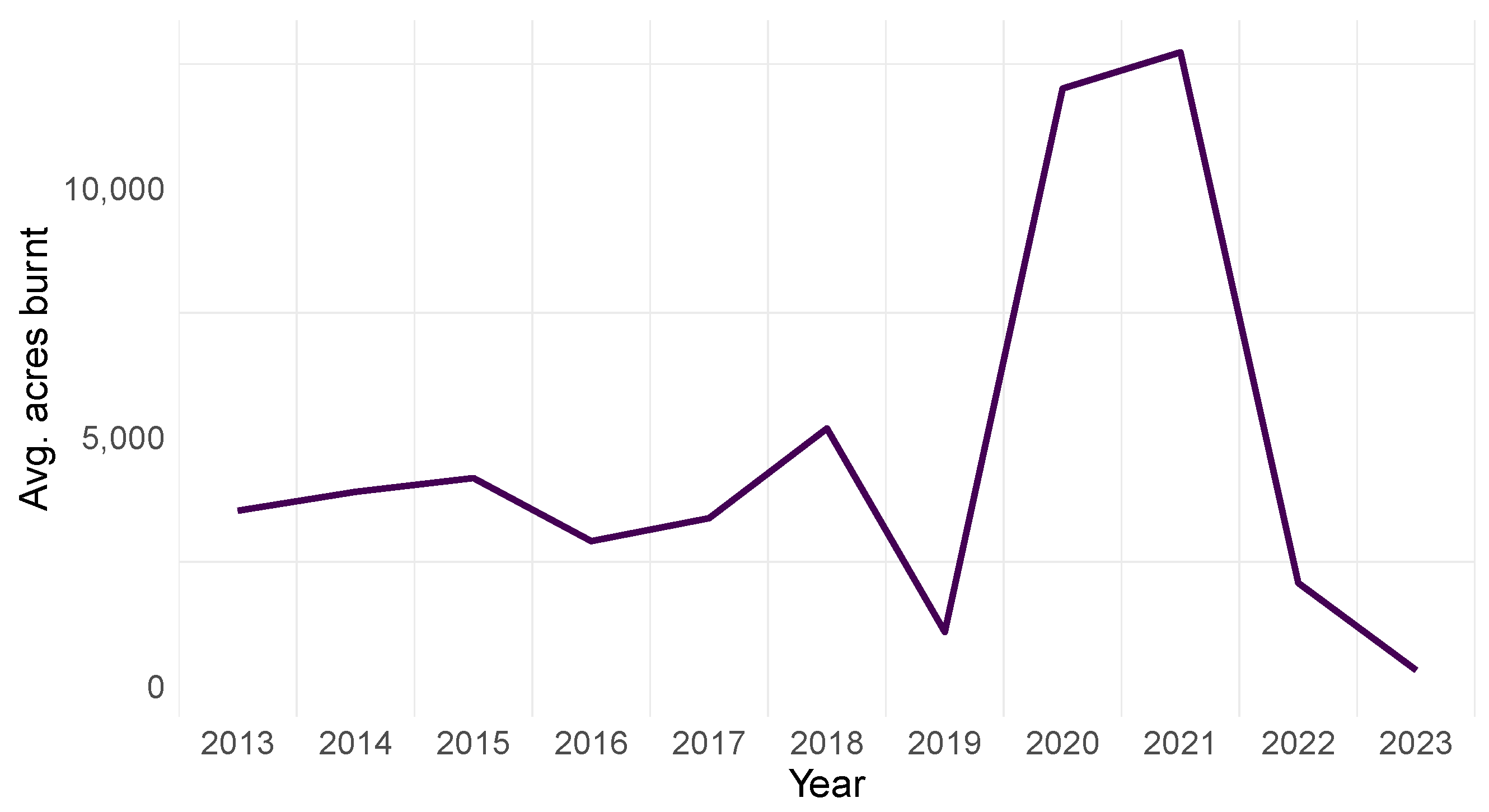
Figure 1. Average acres burned in each year across counties.
J 07 00018 g001
Figure 2. (a) The observed distribution of the wildfire density in California shows right skewness. (b) The log-transformed representation achieves a more symmetric and normalized distribution. (c) The qq plot of the observed data versus a normal distribution shows a clear deviation from normality. (d) The qq plot of the log-transformed data versus a normal distribution depicts a closer fit to normality.
J 07 00018 g002
Figure 3. (a) The spatial distribution of the wildfire density and (b) its log-transformed values across regions in the state of California. Counties with a higher fire density are represented by warmer colors, while cooler colors indicate a lower fire density.
J 07 00018 g003
Figure 4. Posterior credible intervals for mean wildfire density across 57 California counties. The plot aids in classifying counties into top and bottom groups based on mean values. This classification enables us to conduct further analysis of the influential factors within each top and bottom group.
J 07 00018 g004
Figure 5. Posterior predictive check using 100 simulated datasets of wildfire density (yellow) alongside the actual observed data (dark purple).
J 07 00018 g005
Figure 6. Trace plots of factors exhibiting differential effects on top and bottom counties. The trace plots also provide an assessment of the convergence and mixing of the Bayesian regression model for the selected factors.
J 07 00018 g006
Figure 7. Trace plots of factors exhibiting differential effects on top and bottom counties. The trace plots also provide an assessment of the convergence and mixing of the Bayesian regression model for the selected factors.
J 07 00018 g007
Table 1. Summary statistics of variables of wildfire density, average elevation, average temperature, average precipitation, population density, PM10, and SOX from 2013 to 2023.
VariableMeanStd. Dev.MinMax
Wildfire density (acre) 0.688 1.236 0.01 8.71
Elevation (m)666565302216
Temperature (°F) 92.2 6.67 77109
Precipitation (mm) 15.8 7.53 2.51 33
Population 0.586 1.07 0.003 5.19
PM10 ( μ g/m3) 24.2 40.7 1.25 284
SOX (ppb) 1.1 2.459 0.004 13.7
Table 2. Posterior summary of fixed and random effects in the hierarchical ANOVA model.
EstimateStd. Error80% Credible Interval
Fixed Effects
μ −4.050.145(−4.23, −3.86)
Random Effects
σ μ 0.993
σ y 2.11
Table 3. Summary statistics of the Bayesian regression model parameters for the top counties.
TermEstimateStd. Error80% Credible IntervalNeff RatioRhat
(Intercept)−3.6103.79(−8.42, 1.26)0.761.00
SOX−0.0770.07(−0.18, 0.02)0.930.99
PM10−0.0350.03(−0.07, 0.01)0.861.00
Population0.2250.21(−0.05, 0.51)0.750.99
Elevation0.0100.00(0.005, 0.015)0.891.00
Temperature0.0130.03(−0.03, 0.06)0.771.00
Precipitation−0.0500.04(−0.10, 0.01)0.870.99
Sigma0.9600.15(0.80, 1.19)0.661.00
Table 4. Summary statistics of the Bayesian regression model parameters for the bottom counties.
TermEstimateStd. Error80% Credible IntervalNeff RatioRhat
(Intercept)−3.1103.58(−7.74, 1.49)0.671.00
SOX−0.1200.08(−0.23, −0.01)0.651.00
PM100.0010.01(−0.00, 0.01)0.781.00
Population0.4550.25(0.13, 0.78)0.621.00
Elevation0.0030.01(0.000, 0.008)0.820.99
Temperature−0.0230.03(−0.06, 0.02)0.691.00
Precipitation0.0060.02(−0.02, 0.03)0.771.00
Sigma0.6520.10(0.54, 0.80)0.611.00
Disclaimer/Publisher’s Note: The statements, opinions and data contained in all publications are solely those of the individual author(s) and contributor(s) and not of MDPI and/or the editor(s). MDPI and/or the editor(s) disclaim responsibility for any injury to people or property resulting from any ideas, methods, instructions or products referred to in the content.