Article

A Set of State–Space Models at a High Disaggregation Level to Forecast Italian Industrial Production

by
Riccardo Corradini
DIPS Department, Division for Data Analysis and Economic, Social and Environmental Research, ISTAT Italian National Institute of Statistics, 00198 Rome, Italy
J 2019, 2(4), 508-560; https://doi.org/10.3390/j2040033
Submission received: 11 June 2019 / Revised: 8 November 2019 / Accepted: 11 November 2019 / Published: 18 November 2019

Abstract

:
Normally, econometric models that forecast the Italian Industrial Production Index do not exploit information already available at time t + 1 for their own main industry groupings. The new strategy proposed here uses state–space models and aggregates the estimates to obtain improved results. The performance of disaggregated models is compared at the same time with a popular benchmark model, a univariate model tailored on the whole index, with persistent not formally registered holidays, a vector autoregressive moving average model exploiting all information published on the web for main industry groupings. Tests for superior predictive ability confirm the supremacy of the aggregated forecasts over three steps horizon using absolute forecast error and quadratic forecast error as a loss function. The datasets are available online.

1. Introduction

Forecasting industrial production can be a difficult task, but forecasting the sub-components of industrial production at a high disaggregation level can be even more challenging for researchers. This happens because there is some information available at the disaggregated level, and unless it has movements similar to the sub-components, there is the risk of worsening forecast results by simply exploiting the past. Gross data on the Italian Industrial Production Index at a higher disaggregated level are analyzed, exploiting the high correlation with other times series when they are available. Low forecasting performance on average is found when poor or no information is available, consistent with existing literature, but larger improvements were observed for the disaggregated components that face a richer correlation with other variables on their past and on the one-step-ahead prediction.
The related literature (see Bulligan et al. [1]) shows two main sets of models. The first set exploits quantitative data when they are available for the whole index or for its disaggregated components, using regression methods (see, for instance, Marchetti et al. [2] and Bodo et al. [3]) or seemingly unrelated equations methods as in the work of Bruno et al. [4]. The second set exploits so-called common factors that summarize a big set of survey data about industrial production as predictors.
Costantini [5] showed how “The state-space model yields superior forecasts among the factor models” .
To the best of my knowledge, this is the only study that compared the short-term forecasting performance of a naive autoregressive model applied to the Italian Industrial Production Index with a set of state-space models applied to its own main industry groupings.
The effort is motivated to understand the short-term evolution of the Italian economy. It is mandatory to continuously review the estimates to monitor the evolution of quarterly estimates of gross domestic product. There is a trade-off between the need to provide industrial production forecasts closely related with the future evolution of gross domestic product in a short time and doing such a job by exploiting all the information available, as much as possible, with the most suitable econometric tools.
Brunes-Lesage et al. [6] pointed out, when analyzing the French Industrial Production Index, that "The IIP, however, is characterized by a significant publication delay, around 40 days after the end of the reference month for the main European countries, and the first IIP estimations are often revised significantly. Thus, it is less useful for short-term forecasting exercises.” Italian data are not so prone to high revisions, but they are also characterized by the same delay (40 days). The aim of this paper is, therefore, to propose several models designed to forecast the current-month Italian Industrial Production Index (nowcast) using the data listed in Table 1 and to forecast the Italian Industrial Production Index for the next two months after the present time month.
It is shown in further detail using a recursive forecast window starting from January 2001 and moving from January 2008 up to December 2018 that a popular autoregressive of order three over the log seasonal differences benchmark used by Bulligan et al. [1] can be beaten at any disaggregated level. (The Destatis Truck Toll Mileage Index starts from January 2005 and the time series for natural gas from January 2006. Nevertheless, for 2005, we use for natural gas the level given by Italian Ministry of Economic Development. For 2004, we give data about natural gas transported the same monthly percentage of industrial gas registered for the year 2005. For 2001–2004, a naive backcast is carried out for the Destatis Truck Toll Mileage Index using seasonal growth rates of published German Industrial Index of Intermediate Goods. The same strategy is used to backcast the level of production of cars from 2001 to 2007 using consolidated published data from Destatis about production of cars.)
It is shown how aggregating the estimates can obtain more competitive results than the above-mentioned autoregressive model over a three step horizon. We exploit state–space models, focusing mainly on the Truck Toll Mileage Index in Germany (see Askita et al. [7] and Cox et al. [8]) to forecast the Industrial Index of Intermediate Goods and of Capital Goods. Non-durable goods exploit the industrial gas data. Durable goods forecasts exploit the Destatis Truck Toll Mileage Index. Conversely, for the production of electricity, gas, steam and air conditioning supply, due to abundance of daily and monthly Italian data, a set of ad-hoc models at different frequencies is used.
The paper contributes to the research community for the following reasons:
  • A workhouse is beaten by the aggregated model. However, it is still competitive at the third step.
  • A model tailored on Italian holidays history is beaten by the aggregated model.
  • All data are freely available on the web without any restrictions.
  • It uses open source software matrix programming language GNU Octave (see https://www.gnu.org/software/octave/) to enforce transparency of results and to elicit debate among researchers all over the world.
  • For the period before 2015, where it is impossible to use the same fixed weights, a solution is proposed.
  • Computational algorithms and state-space models have never been applied in such a disaggregated context for the Italian Production Index and are not available in standard commercial packages.
  • It shows how it is possible to cast into a state-space model (without imposing restrictions) a vector autoregressive moving average applied to the whole index that exploits as endogenous variables all freely available data at t + 1 on the web concerning Main Industry Groupings disaggregation from January 2001 to December 2018.
  • For the first time, model confidence set procedure of Hansen et al. (see [9]) is applied to Italian Industrial Production Index as well as its sub-components to check the superior predictive ability of aggregated forecasts over a class of competing econometric models.
The remainder of the paper is organized as follows. In Section 2, the data used are presented with the weighted structure of the Italian Production Index. In Section 3, the barebone model and the barebone model enhanced by stochastic regressors are presented. The last one is used for an ad-hoc forecasting study concerning intermediate goods, capital goods and non-durable goods. In Section 4, more recent models are upgraded inserting most of the data freely available on the web used in the disaggregated models. In Section 5, the basic assumptions of the models are inspected. In Section 6, the Kalman filter and the smoothing algorithm are summarized. Section 7 points out the main results using the predictive ability tests ( see Section 3.7). Finally, some conclusions peculiar to the Italian Industrial Production Index are drawn.

2. Data

Figure 1 plots the first log seasonal difference of the following indexes: Industrial Production Index for Intermediate Goods, Industrial Production Index for Capital goods and the German Truck Toll Mileage Index. The last variable is always available at time t + 1. As shown in Figure 2, intermediate goods and capital goods account for 61 per cent of the whole index. Ad-hoc bivariate seemingly unrelated time series equations are used (see example about car drivers’ accidents in the work of Durbin et al. [10] and Section 3.1). The assumption is that these goods are transported in these countries (Italy and Germany) monthly and that there is a relationship among their seasonal growth rates. A similar strategy is considered for the Industrial Production Index of Durable Goods. Bivariate seemingly unrelated time series equations (see Section 3.1) are composed by the German Truck Toll Mileage Index and the Industrial Production Index of Durable Goods. Similarly, for the Industrial Production Index of Non-durable Goods, the seemingly unrelated time series equations are applied to the cumulated monthly data about the industrial natural gas used. On the contrary, a lot of information is ready at the time of the publication on ISTAT’s website concerning production electricity and other sub-components (Figure 3 shows the weights of sub-components). The daily data about consumption of electricity can be cumulated to obtain a preliminary estimate of the monthly data that will be released roughly 15–20 days later. Data about compressed natural gas are less prone to revision and do not differ too much from their preliminary value when cumulated to obtain their monthly value. To obtain an estimate of main industry grouping in the Industrial Production Index of Electricity, gas, steam and air conditioning supply, we must consider four sub-components:
  • Extraction of crude petroleum and natural gas
  • Manufacture of coke and refined petroleum products
  • Electric power generation, transmission and distribution
  • Manufacture of gas; distribution of gaseous fuels through mains.
Most of the time, extraction of crude petroleum happens together with natural gas. Unfortunately, no information was available at time t + 1 for crude petroleum, but we do have daily data about the extraction of natural gas from 2006 up to now. These data are cumulated and inserted into seemingly unrelated time series equations (see, for instance, the example about car drivers killed or seriously injured in Great Britain from January 1969 to December 1984 in [10] and Section 3.1). For t + 2, roughly 25 daily observations (at that time, all monthly data are ready; see Table 1) are always available and are appended to daily time series about the production of compressed natural gas. Manufacture of coke and refined petroleum products is estimated by an autoregressive moving average identification procedure described in Gómez et al. [11] applied to ISTAT’s monthly data. Electric power generation, transmission and distribution is somewhat more complicated.
At time t + 1, production of electricity data from Terna’s website and roughly 25 daily observations of consumption are available because two endogenous variables are available at time t + 1:
  • Consumption of electricity on monthly and daily basis
  • Production of electricity
A conditional vector autoregressive moving average model is used to estimate the index of electric power generation, transmission and distribution at time t + 1. For t + 2 and t + 3, a naive autoregressive model of order three using first seasonal weekly differences applied to daily data about consumption and thermoelectric, national natural gas production and transportation allows us to have more reliable estimates for production of electricity, extraction of petroleum and natural gas and finally distribution of gaseous fuels through mains at time t + 2 and t + 3 (see the Appendix A and Appendix B for further details).

3. Models Used

3.1. Barebone Model

First, our model incorporates regression variables into structural models. Thus, it has the following structure.
Y t = X t β + w t
where w t takes the following general structure (as described by Gómez [12])
w t = p t + s t + u t + v t + e t
where p t is the trend, s t is the seasonal, u t is the cyclical, v t is the autoregressive and e t is the irregular component.
The trend component can be summarized in the following way:
p t + 1 = p t + b t + c t
b t + 1 = b t + d t
where p t is the level and b t is the slope of the trend, and c t and d t are two mutually and serially uncorrelated sequences of random variables with zero mean and variances σ c 2 and σ d 2 , respectively.
The component s t follows trigonometric seasonality
s t = Σ i = 1 [ f / 2 ] s i , t
where f is amounts of observations per year. In our case, f = 12. Each component follows the model
s i , t + 1 s i , t + 1 * = c o s ω i s i n ω i s i n ω i c o s ω i · s i , t s i , t * + j i , t j i , t *
It is assumed that all seasonal components have a common variance, σ i 2 = σ s 2 , i = 1 , 2 , , [ f / 2 ] . To simplify things, the cyclical and autoregressive components are not present. It is straightforward to extend Model 1 into a multivariate one using the Kronecker product.
Thus,
Y t = X t β + W t
where X t is a regression matrix and W t is a multivariate structural model. These last models can be obtained easily from univariate structural models using the Kronecker product (see Chapter 8 of Harvey [13]).
Now let us think for a while X t follows a stochastic process. More accurately, following Gómez [12],
x t + 1 = F x t + G u t
Y t = X t β + H x t + J u t , t = 1 , 2 , , n
where X t is the regression matrix. Since X t follows a stochastic process, the term X t β can be partitioned into two terms.
X t β = M t γ + N t δ = M t γ + ( δ I ) v e c ( N t )
It is possible to rewrite the last equation in the following way
X t β = M t γ + R u t
where M t is a matrix containing the non-stochastic inputs, while u t is the matrix containing the stochastic inputs. Finally, γ and R are the exogenous inputs regressors coefficients and the stochastic input regressors coefficients, respectively.
If we consider the transition equation and the measurement equation for the stochastic inputs u t ,
x u t + 1 = F u x t u + G u v t
u t = X t u β u + H u x t u + J u v t , t = 1 , 2 , , n
With a little bit of algebra combining the model for input with the general model, we obtain the following transition equation and measurement equation
x t + 1 x t + 1 u = F t 0 0 F t u x t x t u + G t 0 0 G t u u t v t
Y t u t = = M t R X t u 0 X t u γ β u + H t R H t u 0 H t u x t x t u + J t R J t u 0 J t u u t v t
The initial conditions for this combined model depend on the initial states x 1 and x 1 u . Since x 1 is known, we have to compute x 1 u . This can be done solving the Lyapunov equation using as input the matrices F u and G u . Further details are indicated in the work by Gómez [12]. To obtain initial conditions for the Kalman filter, the mean and the covariance matrix of the initial state vector x 1 u are needed. If the series is stationary, the mean is obviously zero. As for the covariance matrix, letting Var( x u 1 ) = V, the matrix V satisfies the Lyapunov equation
V = F u · V · F u + G u · G u ;
A more detailed explanation was given by Gómez [14] (Paragraph 4.14.2 about initial conditions in the time invariant case).

3.2. Stochastic Regressors Inside the Barebone Model

The transition and measurement equations shown in Section 3.1 take as given state–space system matrices F t u , G t u , X t u , H t u , and J t u . At time t + 1, the German Truck Toll Index is available. Unfortunately, no information is available for the Italian Industrial Production Index for the manufacture of motor vehicles, trailers and semi-trailers.
Nevertheless, we assume there is a feasible autoregressive moving average seasonally integrated model that could be estimated recursively over time by the automatic identification procedure described by Gómez et al. [11]. For production of cars in Germany, the same procedure is applied. For the sake of interest, we call this system “star system”, where the respective state–space system matrices are cast on the main diagonal to give final results of the aforementioned F t u , G t u , X t u , H t u , and J t u . Figure 4 shows the flowchart of the computer source code used to obtain the in-sample state–space stochastic input system.
Once the Italian and German data are loaded in memory, the automatic identification procedure stores the results about their respective state–space forms. If the algorithms crashes, it is mandatory to use the logarithmic transformation (see Gómez [15]) and the property of log normal distribution to bring those data on the original level if it is desirable. Finally, the matrices are cast on the main diagonal of F t u , G t u , X t u , H t u , and J t u .
Figure 5 shows how the computer code mentioned above is cast into the bivariate SUTSE with Italian Industrial Production Index for Capital Goods and the German Truck Toll Index.
The same system may be applied to Italian Industrial Production Index of Intermediate Goods and the Truck Toll Index. As stochastic regressors, we use the commercial vehicle registration in Germany and the commercial vehicle registration in Italy. In this last case, both regressors are available at time t + 1, while in the case for capital goods only the level of production of cars in Germany is present. The same gearings are applied for the system about non-durable goods and natural gas for industrial use. We use as stochastic regressors consumption of electricity and commercial vehicle registration in Italy always available at time t + 1. The Kalman filter log likelihood estimation does not force us to estimate the whole concatenated system. Once the bivariate SUTSE is estimated, we only have to combine this system with the star system and finally apply the Kalman Filter’s smoothing recursion (see Gómez [14]) to obtain the new forecasts with stochastic exogenous regressors for Italy and Germany.

3.3. Mixing Stochastic Regressors with Barebone Model due to Failure in Convergence

Sometimes it happens that the star system (see Figure 4) fails to converge due divergence between the two series. For instance, production of cars and trucks in Italy during the month of August is less labor-intensive than in Germany. Consequently, in certain months, such as August 2009, in a period of crisis, the divergence between German production of cars and the Italian twin is even more marked and the Kalman filter algorithm fails to converge in the star system. During the recursive estimation in the case of failure of convergence, a rollback strategy to the barebone model has been implemented. The same strategy applies to the enhanced barebone model for intermediate goods and for non-durable goods.

3.4. Long Weekends

During some months, there are fixed holidays on Tuesdays or Thursdays. A typical example is the Immaculate Conception holiday on the 8th of December. Many workers requested to go on holiday on the 7th of December 2015. In this way, they used four days (Saturday, the 5th of December; Sunday, the 6th of December; Monday, the 7th of December; and the day of the Immaculate Conception). The raw data about the Industrial Production Index are affected by such a slowdown on Monday, the 7th of December. Nevertheless, ISTAT does not consider the group of people who do not work during that day. The calendar and seasonal adjustment is strict. Alternatively, most of the times, the calendar adjusted time series are more predictable than gross ones.
Time series not affected by strikes or unexpected holidays could be predicted more easily than gross ones. To tackle this problem, on the calendar from the 1st of January of 2001 for the following days are traced:
  • New Year’s Day
  • Epiphany: the 6th of January
  • Italian Republic day: the 2nd of June
  • Immaculate Conception: the 8th of December
  • International Workers’ Day: the 1st of May
To trace the long weekends, the following strategy is proposed:
  • For New Year’s Day, Epiphany, Italian Republic day, and Immaculate Conception, find the years when they happen on Tuesdays and Thursday.
  • Create a binary dummy variable to inform the model there will be a discrepancy between what it expects and what happens in the real world and place it on Mondays or Fridays for daily data.
  • For the 1st of May, let the computer decide if the month of April is affected when Labour Day happens on Tuesday or Thursday. The same algorithm is applied to New Year’s Day.
  • Compute dummy variables for the months over the years detected from the procedure mentioned above.

3.5. Long Weekends and Airline Model with No Logarithmic Transformation

To exploit the aforementioned dummies (see Section 3.4), I inserted them into a popular airline model with no logarithmic transformation.
( 1 B ) ( 1 B 12 ) y t = ( 1 θ B ) ( 1 Θ B 12 ) ϵ t + β X t
where B is the backshift operator and X t contains number of workings days in Italy on monthly basis and the whole set of long weekend dummies. Table A19 shows the final results at the end of the sample. This naive model is inserted into the forecasting competition (see Section 7).

3.6. Benchmark Model, MAE and RMSE over Seasonal Differences

Δ 12 l o g ( y t ) = j = 1 3 Δ 12 γ j l o g ( y t j ) + ϵ t
Equation (18) describes the autoregressive benchmark used by Bulligan et al. [1]. The Mean Absolute Error (MAE) is computed over Δ 12 l o g ( y t ) . It is given by the following formula:
M A E = 1 n j = 1 n | Δ 12 l o g ( y t ) Δ 12 l o g ( y t ) ^ |
where y ^ is the forecast by the model chosen and n is given by the end of the sample. To ease the comparison, the following ratio is used during the recursive experiment:
I M A E = M A E D I S M A E B E N
where M A E B E N is approximately Equation (18) and M A E D I S is given by the model chosen for the disaggregated component. Unless specified, M A E D I S uses the barebone model shown in Section 3.1.
On the same path, the Root Mean Squared Error (RMSE) is again computed over Δ 12 l o g ( y t ) and is given by the following formula:
R M S E = 1 n j = 1 n [ Δ 12 l o g ( y t ) Δ 12 l o g ( y t ) ^ ] 2
The ratio between the disaggregated model forecast and the benchmark model is used:
I R M S E = R M S E D I S R M S E B E N

3.7. Tests of Predictive Accuracy

As Bruno et al. [4] for h-step ahead forecasts, we use the modified Diebold–Mariano statistic:
D M * = n + 1 2 h + n 1 h ( h 1 ) n 1 2 d ¯ n 1 2 π f d ( 0 ) ^
where n = 36, d ¯ = n 1 t = 1 n d t , d t = g ( e 1 t ) g ( e 2 t ) is an arbitrary function of the forecasting errors from model i 1 , 2 , and f d ( 0 ) ^ is a consistent estimate of the zero-frequency spectral density of d t .
When performing tests of forecast encompassing, d t becomes d t = e 1 t ( e 1 t e 2 t ) (see [16]) under the alternative, Forecast 1 could be improved by incorporating some of the features present in Forecast 2. When comparing forecasting accuracy, in this paper, we use d t = | e 1 t | | e 2 t | and d t = e 1 t 2 e 2 t 2 .
Albuquerque [17] showed that: “The Hansen’s Test of Superior Predictive Ability can be addressed by testing the null hypothesis that the benchmark is not inferior to any alternative forecast. We seek a test of the null hypothesis that the benchmark is not inferior to any of the alternatives.” In other words,
d k , t = ( d 1 t d m t )
where the vector d k , t is the vector of stacked relative alternatives.
Hansen test works under the assumption that model k is better than the benchmark if and only if equation E ( d k , t ) > 0 .
The Hansen [18] superior predictive ability test assumes that d t is (strictly) stationary and second finite moment (to be possible to apply the Central Limit Theorem).
In this case, the asymptotic null distribution is:
n 1 2 d ^ N k , t ( 0 , Ω ^ )
At this point, all essential aspects of our framework are identical to those of [19] Reality Check (RC). White, H. [19] proceeded by constructing the RC from the test statistic:
T n R C = m a x ( n 1 2 ) d ^ 1 , , d ^ m
where d ^ k is the sample mean associated with the kth model and Ω is a consistent estimator of the variance and covariance matrix.
Berardi et al. ([20]) summarized the model confidence set procedure (see Hansen et al. [9]): The procedure starts from an initial set of models M 0 of dimension m encompassing all the model specifications M ^ 0 and delivers for a given confidence level 1 α , a smaller set, the superior set of models, SSM, M ^ 1 α * of dimension m * m . The best scenario is when the final set consists of a single model, i.e., m * = 1 . Formally, let d i j , t denote the loss differential between models i and j:
d i j , t = l i , t l j , t , i , j = 1 m , t = 1 , , n
and let
d i · , t = ( m 1 ) j M d i j , t , i = , m
be the simple loss of model i relative to any other model j at time t. The EPA hypothesis for a given set of models M can be formulated in two alternative ways:
H 0 , M : c i , j = 0 , forall i , j = 1 , 2 , , m H A , M : c i , j 0 , for some i , j = 1 , 2 , , m
or
H 0 , M : c i , j 0 , forall i = 1 , 2 , , m H A , M : c i , j = 0 , for some i = 1 , 2 , , m
where c i j = E ( d i j ) and c i = E ( d i ) are assumed to be finite and not time dependent. According to Hansen et al. ([9]), to test the two hypotheses above, the following two statistics are constructed:
t i j = d ¯ i j v a r ^ ( d ¯ i j ) and t i · = d i ¯ v a r ^ ( d ¯ i ) i , j M
where d i ¯ = ( m 1 ) 1 j M d i j ¯ is the simple loss of the ith model relative to the average losses across models in the set M, and d i j ¯ = ( m ) 1 t = 1 m d i j , t , t measures the relative sample loss between the ith and jth models, while v a r ( d ¯ i , · ) ^ and v a r ( d ¯ i j ) ^ are bootstrapped estimates of v a r ( d ¯ i , · and v a r ( d ¯ i j ) , respectively. As discussed by Hansen et al. (see [9]), the two EPA null hypotheses presented in Equation (28) map naturally into the two test statistics:
T R , M = m a x i , j M | t i , j | and T m a x , M = m a x i M t i · ,
where t i , j and t i · are defined in Equation (29). The test statistics defined in Equation (30) can be used to test the two hypotheses in Equation (28), respectively. Since the asymptotic distribution of the two tests statistic is nonstandard, the relevant distribution under the null hypothesis is estimated using a bootstrap procedure similar to that used to estimate v a r ( d ¯ i , · ) and v a r ( d ¯ i j ) . The MCS procedure consists of a sequential testing procedure that eliminates the worst model at each step, until the hypothesis of equal predictive ability (EPA) is accepted for all the models belonging to the SSM. The choice to eliminate the worst model was carried using an elimination rule that is coherent with the statistic test defined in Equation (29):
e m a x , M = a r g m a x i M d ¯ i , · v a r ^ ( d ¯ i , · ) and e R , M = a r g m a x i M { s u p j M d ¯ i j v a r ^ ( d ¯ i j ) }
respectively.
In summary, the MCS procedure to obtain the SSM consists of the following step:
Step 1.
Set M = M 0 .
Step 2.
Test for EPA hypothesis: if EPA is accepted, terminate the algorithm and set M 1 α * = M , otherwise use the elimination rules defined in Equation (31) to determine the worst model.
Step 3.
Remove the worst model, and go to Step 2.
This paper uses the MCS procedure (see Hansen et al. [9]) and test for superior predictive accuracy of Hansen (see [18]) implemented by Sheppard (see [21]) available for MATLAB.

4. VARMA Applied to the Whole Index

This section describes the model applied to the whole index in VARMA state–space form. The German Truck Toll Index is backcast using a naive reconstruction from 2001:01 to 2004:12. To this series is assigned the same seasonal growth rate of the consolidated published time series of Industrial Production Index for Intermediate Goods in Germany. In this way, endogenous variables can be employed in the following time series:
  • Industrial Production Index in Italy
  • Consumption of electricity in Italy
  • Truck Toll Index in Germany
Unfortunately, the time series data on natural gas for industrial use are not available before 2005:01. It is not possible to compute a naive backcast due to lack of information up to 2001:01. Since the last two variables have always been available at time t + 1, they are inserted in state–space form of the Kalman filter. The following general procedure is employed with an expanding window starting from 2001:01 to 2008:01. The last one is expanded at every step of the recursive estimation up to 2018:12. The mandatory steps to estimate this type of VARMA model are given below:
  • Identify the VARMA model with an iterative likelihood-ratio test procedure (see Gómez [12] for an analytical description).
  • Carry out a preliminary estimation of the parameters by the Hannan–Rissanen method (see Gómez [12] and Hannan et al. [22]).
  • Refine the estimation using the conditional method described by Lütkepohl ( see [23]), Reinsel [24]) and Gómez (see [12,14] for the implementation).
  • Cast the new parameters into state–space form.
  • Use the Kalman filter for maximum likelihood estimation.
  • Perform diagnostic testing.
  • Estimate forecast using the information about other endogenous variables available at time t+1.
The aforementioned procedure can be applied to any VARMA process of any given dimension. This simplified VARMA model is used to compare the forecast with the aggregated model by means of the model confidence set (see Hansen et al. [9]). The Supplementary Materials presents two videos (see Supplementary Video S1 and Supplementary Video S2) that show the evolution of the p-values of the multivariate Q-statistic (see Gómez [12]) applied to vectorized residuals and squared vectorized residuals over 36 lags applied to the basic model. A similar model that does not exploit public available data (i.e., railway transportation data provided by Trenitalia Cargo and monthly level of temperatures) was described by Ventura et al. (see [25]) and does not exploit Kalman filtering. Their model is summarized by the following nested models:
y t = i = 1 p ϕ i y t 1 + j = 0 q γ j z t j + ϵ t
y t = i = 1 p ϕ i y t 1 + j = 0 q γ j z t j + ζ j F t + η t
where F t represents R × 1 vectors of factors obtained via cross-validation, and ζ is a conformable coefficient vector. Since the block intermediate plus capital and electricity account roughly for seventy per cent in terms of weights about the whole index (see Figure 2), this study focuses only on the survey data concerning non-durable goods. In this way, it focuses on ninety per cent of all the information available on the web for the whole index from January 2001 up to now. The factors are not extracted and all the raw data on surveys are inserted as they are published (not seasonally adjusted, as by Costantini [5] or log-linearised as by Bruno et al. [4] and, again, by Ventura et al. [25]). The Italian Industrial Production Index, the Truck Toll Index and the consumption of electricity are expressed as logarithms. Preliminary analyses show that the presence of unit roots at some seasonal frequencies cannot be excluded. Accordingly, all variables are transformed through seasonal differencing. Finally, the first difference filter is applied to seasonal differenced variables to achieve stationarity for energy and Truck Toll Index and Italian Industrial Production Index. Table 2 presents the survey data list as in the work of Costantini ([5]) concerning non-durable goods. These data are used in first difference according to the well-known general representation of the VARMA model:
Φ ( B ) Y t = Θ ( B ) A t + β X t ,
Y = Y 1 Y 2
where Y 1 = Δ Δ 12 l o g ( y t ) is the vector containing the variables listed in Table 2 for the hard data and Y 1 = Δ y t for the survey data about non-durable goods. Finally, X t contains Δ Δ 12 l o g ( w d t ) , where w d t is the number of workings days in Italy and a couple of level shifts detected by SSSMATLAB for Italian Industrial Production Index. These thirteen endogenous variables are estimated recursively over the three-step horizon. Step 1 includes studying all the information already available for the other twelve variables. For the other two steps, the forecast is unconditioned. Figure 6, Figure 7 and Figure 8 show the results of the Durbin–Watson test on autocorrelation, the Harvey test on heteroskedasticity and the Bowman–Shenton test for normality testing. It can be seen that the Durbin–Watson is largely above five per cent for the whole sample, and the heteroskedasticity test rejects the null hypothesis of no heteroskedasticity of the residuals at the five per cent level of significance for the whole of 2013 and the result of the Bowman–Shenton test on normality testing is negative, rejecting the null hypothesis at five per cent level of significance starting from the beginning of 2013 up to the end of the sample. Likewise, global crisis is hardly detected around August 2009 and, again, the test has roughly one year of rejection between the second half of 2011 and the first half of 2012.
Adding the whole set of endogenous variables for non-durable goods (soft data) from the ISTAT survey apparently does not improve the overall picture (see Table 3). In fact, Table 4 shows that the modified Diebold–Mariano test (see Harvey et al. [16]) strongly rejects the null hypothesis of equal forecast accuracy compared to the benchmark of Bulligan et al. ([1]) on the first and third steps. In addition, at the second step, the p-value of the encompassing test strongly rejects the null hypothesis in August 2009, a peak of absolute error of the benchmark is observed. The diagnostic does not show an improvement with respect of the basic VARMA model using the hard data. Figure 9 shows the DW test for this VARMA using both hard and soft data for non-durable goods. Figure 10 shows the results of Normality testing. Figure 11 shows the Harvey test using both hard data and soft data for non-durable goods.
Table 5 shows how the second VARMA greatly benefits from the information already available at time t + 1 for hard and soft data (i.e., all the p-values are below the five per cent significance). At time t + 2, this gap is evident to strongly accept the null hypothesis that VARMA using just the hard data encompasses the model that uses both hard and soft data for non-durable goods. At time t + 3, the gap between the huge VARMA and hard data VARMA shrinks again. Again, at t + 1, the null hypothesis of encompassing both the peak of the crisis (i.e., August 2009 under two per cent significance) and the end of the sample (below one per cent significance) are rejected.

5. Recursive Diagnostics of Disaggregated Models

This section presents the results of diagnostics related to the distinct disaggregated model used. For intermediate goods, we consider the regressors for following time series: (1) working days in Italy and Germany; (2) a linear trend; (3) a series of outliers and the level shift identified on the overall sample before the computer started the recursion by SSMMATLAB plus a level shift to inform the computer about our naive backcast for the period 2001:01–2004:12; (4) the level of registration of commercial vehicles in Italy; and (5) the level of of registration of commercial vehicles in Germany.
Figure 12 plots the difference between the recursive Bayesian information criterion (see Gómez [12] for a description of the diagnostics and Schwarz [26]) of the barebone model for intermediate goods and the enhanced model for intermediate goods. The Bayesian information criterion of the enhanced model is always inferior.
At the beginning of the recursive experiment, between January 2008 and January 2009, the enhanced model did not show its own supremacy. From the beginning of 2009, the situation constantly improved in favour of the enhanced model. In other words, starting from 2009, the new regressors had an upward contribution waving around a linear trend. This hints the use of the enhanced model as a long-run solution due to the growing importance of commercial vehicles registration in both countries to understand the long-run evolution of industrial production. On the basis of this evidence, we now focus on the diagnostics of this enhanced model for intermediate goods. Table A8 shows the final results at the end of the sample (December 2018). We see that the regressor coefficients of the stochastic regressors are statistically significant, and we strongly reject the null hypothesis on the basis of the t-values over time. The Supplementary Materials present a video (Supplementary Video S3) showing how the aforementioned p-values of the stochastic coefficients are constant and stable. Surprisingly, the impact of working days in Germany is superior to the impact of working days in Italy on the Italian Industrial Production Index of Intermediate Goods. For the Truck Toll Index, the difference is less outstanding. The coefficient of the linear trend shows a negative impact over the Italian data while its twin for the Truck Index shows a positive impact. This again does not come as a surprise given the persistent upward trend of the German data. Similar conclusions might be drawn from the coefficients of commercial vehicles registrations for both the countries. The Bowman–Shenton test (see Bowman et al. [27] and Figure 13), with unique exceptions towards the end of 2008 and the end of 2017, is always above the five per cent rejection area of the null hypothesis.
Figure 14 shows the p-values of the Durbin–Watson statistics (see Durbin et al. [28,29]) for the enhanced barebone model of intermediate goods. At the bottom of the graph, the straight red line denotes 0.05 line significance. The null hypothesis of no autocorrelation of the residual was strongly accepted during the whole experiment. The results of heteroskedasticity test of Harvey are more unstable at the beginning of the experiment (see Figure 15) (see Harvey [13], p. 259).
Due to global economic crisis, the test is rejected at five per cent significance level for the years between 2009 and 2011. Nevertheless, the model began recovering from 2012 with an upward trend and then waved roughly from 2016 below the 0.2 line. Using the sample autocorrelations of the residuals and squared residuals, it is possible to show the evolution of Q-statistics for over 36 lags. The Supplementary Materials present two videos (Supplementary Video S4 and Supplementary Video S5) to show the movements of the p-values for both the tests over the 0.05 significance. It is possible to ensure that both the tests are hardly rejected over 36 lags and over time after the global crisis.
Again, the enhanced model shows its own supremacy in terms of the Bayesian information criterion for capital goods.
A direct comparison of Figure 12 and Figure 16 shows how the difference in terms of the Bayesian information criterion is even more marked for capital goods than for intermediate goods. Even in this case, the enhanced model is the focus of this study. Harvey’s test for heteroskedasticity has hardly been rejected from January 2008 up to the second half of 2016 (see Figure 17). The p-value of this test still waves around the significance red line for the remainder of the sample. Even more satisfying are the results of Bowman–Shenton statistics (see Bowman et al. [27] and Gómez [12]) over the whole experiment (see Figure 18). On the same line, the lack of autocorrelation between the residuals on the basis of the Durbin–Watson’s p-value is depicted in Figure 19. In the Supplementary Materials, the flow of the Q-statistics over the three dimensions applied to the residual and the squared residuals can be seen (i.e., Supplementary Video S6, Supplementary Video S7). Even in this case, we can see that, in most instances, the p-values waved far from the bottom. Table A10 shows the values of the parameters estimated by the Kalman filter by maximum likelihood at the end of the sample. Both endogenous variables are more significantly affected by the level shift detected from 2009:02 than the other ones previously detected by SSSMATLAB. The coefficient about working days can almost be swapped in terms of value between the level for Italy and Germany. The working days in Germany have a positive effect over the Italian data while the working days in Italy have a slight negative effect over the German data. This can be explained by geographical reasons. Many firms concerning capital goods located in the north of Italy may be connected with German firms in the south of Germany. Thus, when Italians work more because they have more working days in a month, they may influence German workers. In addition, the linear trend has a stronger effect in Germany than in Italy. The contribution of commercial vehicle registration in Italy is more marked for German data than for Italian data. The picture is reversed for German data. The Supplementary Materials provide the evolution of p-values and t-statistics over time to check the parameters’ stability (i.e., Supplementary Video S8). It can be seen that the overall picture of the parameters is stable over time.
Table A14 displays the results of maximum likelihood estimation at the end of the sample for the barebone model for durable goods. The level shifts from 2008:1 are in the group of the most significant coefficients among the selected variables. Figure 20, Figure 21 and Figure 22 summarize the results of the recursive Durbin–Watson test for autocorrelation, Bowman–Shenton test for normality and Harvey test for heteroskedasticity. Once again, the null hypothesis is not rejected. In term of weights (see Figure 2), the results concerning the Italian Industrial Production Index of Non-Durable Goods are more relevant. Figure 23 shows the difference between the Bayesian information criterion of the barebone model and the enhanced model for non-durable goods. The difference between the other aforementioned figures (see Figure 12 and Figure 16) about the intermediate and capital is more evident. Nevertheless, even for non-durable goods, the enhanced model shows a better BIC for the major part of the experiment. Two of the three usual tests for normality (see Figure 24, Figure 25 and Figure 26) do not show a unique convincing picture for the last three years. Table A15 shows the results at the end of the sample for the enhanced model for non-durable goods. It can be seen that the impact and the statistical significance of consumption of electricity is higher for Industrial Production Index of Non-durable Goods than for natural gas for industrial use. Conversely, the impact of commercial vehicle registration in Italy is higher in natural gas for industrial use. The video in the Supplementary Materials concerning the p-values and t-statistics’ evolution over time (see Supplementary Video S9) shows more movements than the enhanced model for intermediate goods and than the model for capital goods.
Figure 25 shows the p-values of Durbin–Watson statistics (see Durbin et al. [28,29]) for the enhanced barebone model of non-durable goods. At the bottom of the graph, the straight red line denotes 0.05 line significance. The null hypothesis of no autocorrelation of the residual is strongly accepted during the whole experiment. Towards the end of the second half of 2016 (see Figure 26), the results of heteroskedasticity test of Harvey (see Harvey [13], p. 259) are less stable than the past.

6. Forecasting Study and Evaluation

6.1. Kalman Filter and State–Space Models

As indicated in Chapter 4 of Gómez [14], using the measurement equation and the transition equation shown in Section 3.1, the Kalman filter is given by the following recursion
E t = Y t H t x ^ t | t 1 , , Σ t = H t P t H t + R t K t = ( F t P t H t + G t S t ) Σ t 1 , , x ^ t + 1 | t = F t x ^ t | t 1 + K t E t
P t + 1 = F t P t F t + G t Q t G t ( F t P t H t + G t S t ) = ( F t + K t H t ) P t F t + ( G t Q t K t S t ) G t ,
initialized with x ^ 1 | 0 = a and P 1 = Ω . Again, Gómez [14] showed the log-likelihood
l ( Y ) = c o n s t a n t 1 2 1 σ 2 t = 1 n E t Σ t 1 E t + t = 1 n l n | σ 2 Σ t |
and that maximizing the log-likelihood above is equivalent to minimizing the following non-linear sum of squares
S = t = 1 n | σ t | 1 2 n p t = 1 n e t e t t = 1 n | Σ t | 1 2 n p
The specialized software described by Gómez [12,15] handles this special form of S where e t = Σ t 1 2 E t .

6.2. Smoothing

Gómez [14] (Section 4.10) showed the following recursions are used for t = n , , 1
( L t , λ t ) = Z t Σ t 1 ( E t , e t ) + K p , t ( L t + 1 , λ t + 1 ) , , Λ t = Z t Σ t 1 Z t + K p , t Λ t + 1 K p , t
where K p , t = T t K t Z t , initialized with ( L n + 1 , λ n + 1 ) = ( 0 , 0 ) and Λ n + 1 = 0 . Letting α ^ t | n = E ( α t | Y ) be the orthogonal projection of α t onto Y and P ^ t | n = M S E ( α ^ t | n ) for t = n , , 1 , the fixed interval smoother is given by
α ^ t | n = U t , α t | t 1 + P t L t , λ t γ ^ n + 1 , 1
P t | n = P t | n + ( P t L t U t ) n + 1 P t L t U t σ ^ 2
where γ ^ n + 1 and n + 1 are the GLS estimator of γ for Y and its MSE.

6.3. Some Reflections over the Period before December 2014

The period from January 2001 to December 2014 requires an ad-hoc treatment to compare the performance of the disaggregated composed model and a naive benchmark model, i.e., autoregressive model of order three over the log seasonal differences of the whole index.
For this, two issues need to be tackled:
  • backcast consumption of electricity daily data from 2006 to 2013 exploiting the compressed natural gas for thermoelectricity daily data; and
  • since the weight of every sub-component is not fixed for this period, e.g. from January 2015 up to present time (i.e., they were rebuilt in terms of growth rate at the cost of fixed weight base year structure), it is mandatory to compute the discrepancy between the data published and the data obtained, holding the structure of base year weight (i.e., 2015) constant.
    I P I = α I P I x + β I P I y + d i s c r e p a n c y : d i s c r e p a n c y = d i s c r e p a n c y α + d i s c r e p a n c y β ; d i s c r e p a n c y α = d i s c r e p a n c y · α ; d i s c r e p a n c y β = d i s c r e p a n c y · β

6.4. Forecasting Competition for the Enhanced Model Applied to Intermediate Goods, Capital Goods and Non-Durable Goods

It can be argued that Equation (33) faces the following problems:
  • It uses log transformation.
  • It applies the difference operator twice (first time with respect to the season and the second with respect to the year).
See Section 3.1 and Gómez [12] for a description of SUTSE models (SSSMATLAB computer programs are available from the author upon special request).
Table 6 outlines the results of the model confidence set procedure (see Hansen et al. [9]) at the end of the sample using absolute error as the loss function. The supremacy of the enhanced model is shown in the last line of the table (see ENHTTMI). The difference with its competitors shrinks at Step 3. This is probably due to lack of information. This picture is confirmed looking at Table 7. Table 8 outlines the results of the model confidence set procedure at the end of the sample using squared error as the loss function. In this case, the difference with respect to the simple barebone model competitors (in particular, BBTTMI and BBLCVSP) is stable over time. Table 9 shows the same results only at Steps 2 and 3. Table 10 shows a restricted group of model with similar results for capital goods. Once again, the choice of stochastic regressors enhanced the model in an upper position. This results is more important compared to the one shown in Table 11. On this table, the victory of the enhanced model is not evident on the sample. On the other hand we are interested if the victory of the enhanced model is statistically significant, so the results of the previous table are more convincing for us. Within the ratios of root mean square errors (RMSE) with respect to the benchmark of Bulligan et al. ([1]), Table 12 shows that within the sample the difference is not so significant. Table 13 shows that the use of stochastic regressors over the three-step horizon is the winning choice on the side of model confidence set procedure for capital goods.
The picture is somewhat more linear for the enhanced model for non-durable goods using absolute error and quadratic error as loss function for model confidence set procedure (see Table 14 and Table 15) and the IMAE (Table 16) and IRMSE (Table 17) tables.

7. Results and Discussion

Table 18 summarizes the performances of the models applied to the disaggregated components mentioned in Figure 2 using the IMAE mentioned in Section 3.7. Table 19 summarizes the results of the modified Diebold-Mariano test mentioned in Section 3.7 using as loss function absolute forecast error. On the same path Table 20 focuses on the the IMAE concerning the subsample from January 2015 up to December 2018, while Table 21 points out the results the modified Diebold-Mariano test mentioned in Section 3.7 using as loss function absolute forecast error for the subsample from January 2015 up to December 2018. Table 22 shows the performances of the models applied to the disaggregated components mentioned in Figure 2 using the IRMSE mentioned in Section 3.7. Table 23 focuses on the results the modified Diebold-Mariano test mentioned in Section 3.7 using as loss function quadratic forecast error. Again on the same path Table 24 focuses on the the IRMSE concerning the subsample from January 2015 up to December 2018, while Table 25 points out the results the modified Diebold-Mariano test mentioned in Section 3.7 using as loss function quadratic forecast error for the subsample from January 2015 up to December 2018.
An expanding window starting from January 2001 and moving from January 2008 to December 2018 is considered. (The dataset is updated on a monthly basis and is not prone to high revisions (see dati.istat.it/). It was downloaded on 8 February 2019.)
The disaggregated model outperforms the benchmark at Step 1 and is still competitive at Step 2 due to the information available from the energy sector and, at Step 3, still holds due to good performance of the intermediate, capital and non-durable goods. Disaggregating simply using the past does not help. The line IPI-BENAGG shows that aggregating the benchmarks applied to the sub-components does not change the situation. This concept is confirmed looking at the results shown in Table 26, Table 27, Table 28, Table 29, Table 30, Table 31 and Table 32. Using 25 days of data, we achieved better results at Step 2 and still competitive results due to an-hoc identification production on daily data (see Gómez et al. [11]). Table 27, Table 29, Table 31 and Table 33 summarize the results of the modified Diebold–Mariano test mentioned in Section 3.7 for electricity.
We see that especially for the subsample from January 2015 to December 2018 the sub-component in charge of production of electricity can accept the null of equal forecast accuracy, especially at Step 2. Finally, it recovers at Step 3, where we may reject the null hypothesis of equal forecast accuracy at ten per cent significance. The low performance of IPI-PETROL is due to the lack of information for this sub-component. We can accept the null hypothesis of equal forecast accuracy with respect to the benchmark of using different loss functions only for durable goods. Given their low importance in terms of weights, the overall impact is negligible.
Finally, the model confidence set procedure described in Section 3.7 can be used to make comparison with all the models mentioned in this paper. Using the absolute forecast error as a loss function (see Table 34), the aggregated model on average is found to be the best, and there are no competitors. Using the quadratic forecast error as a loss function (see Table 35), the difference shrinks due to lack of information. Nevertheless, the aggregated model is still the best over the three-step horizon.

8. Conclusions

We evaluated the gains in the information from the highest disaggregation level at time t + 1 and time t + 2. Using statistical inference, we found that, for enhanced barebone models for intermediate goods, capital goods were the best in terms of superior predictive ability with respect to the set benchmark as well as other combinations of the barebone model not using the German Truck Toll Index. The barebone model for durable goods is the weakest model compared to the set benchmark due to lack of information concerning this index. Nevertheless, its relative weight (four per cent ) is negligible. We found that, using a quadratic forecast error loss function, we accept the null hypothesis of equal forecast accuracy between the enhanced model for non-durable goods and the benchmark in the subsample from January 2015 up to December 2018 (see Table 25). This result for non-durable goods is not confirmed (see Table 21). On average, the enhanced model for non-durable goods is still competitive over three steps horizon.
Of course, when the forecasting errors propagate over time, even a naive autoregressive model (see Section 3.5) is competitive with a disaggregated one (see Steps 2 and 3 of Table 35). Nevertheless, guessing the proper data generating process inside the main components allows us to shrink the forecast bands, even on the third-step horizon (see Table 34 and Table 35), where some information is available.

Supplementary Materials

The following are available online at https://www.mdpi.com/2571-8800/2/4/33/s1, Video S1: Evolution of Q-statistics and p-values over time and over 36 lags applied to vectorized residuals of Varma Basic Model , Video S2: Evolution of Q-statistics and p-values over time and over 36 lags applied to squared vectorized residuals of Varma Basic Model, Video S3: Evolution of t-statistics and p-values over time of regressors coefficients of Enhanced Model for intermediate goods, Video S4: Evolution of Q-statistics and p-values over time and over 36 lags applied to vectorized residuals of of Enhanced Model for intermediate goods , Video S5: Evolution of Q-statistics and p-values over time and over 36 lags applied to squared vectorized residuals of of Enhanced Model for intermediate goods, Video S6: Evolution of Q-statistics and p-values over time and over 36 lags applied to vectorized residuals of of Enhanced Model for capital goods , Video S7: Evolution of Q-statistics and p-values over time and over 36 lags applied to squared vectorized residuals of of Enhanced Model for capital goods, Video S8: Evolution of t-statistics and p-values over time of regressors coefficients of Enhanced Model for capital goods, Video S9: Evolution of t-statistics and p-values over time of regressors coefficients of Enhanced Model for non-durable goods.

Funding

This research received no external funding.

Acknowledgments

The views expressed in this paper are those of the author and do not represent those of the ISTAT. This article describes personal research in progress by the author and is published to elicit comments, to further debate and call for material collaboration in future developments of this research project. Thanks are given to all participants the 35th International Symposium on Forecasting–Riverside–California, U.S.A. Thanks are given to Fabio Bacchini and Giancarlo Bruno from Istat. I am grateful to Victor Gómez, statistician and technical advisor at the Spanish Ministry of Finance and Public Administrations in Madrid, for his constant effort to let people understand the inner gearings of the Kalman filter.

Conflicts of Interest

The author declares no conflict of interest.

Abbreviations

The following abbreviations are used in this manuscript:
IPIItalian Industrial Production Index
LCV-SUMSum of the level of registration of light commercial van over Germany, Italy, France and Spain
LCV-GERLevel of registration of light commercial vehicles in Germany
LCV-ITALevel of registration of light commercial vehicles in Italy
LCV-FRALevel of registration of light commercial vehicles in France
LCV-SPAINLevel of registration of light commercial vehicles in Spain
SUTSESeeminly unrelated time series equations
VARMAVector autoregressive moving average
IPI-AGGForecast obtained by aggregating sub index forecasts
IPI-AGGFROM201501Forecast obtained by aggregating sub index forecasts from January 2015
IPI-AGGForecast obtained by aggregating naive benchmark sub index forecasts
IPI-INTItalian Industrial Production Index of Intermediate goods
IPI-CAPItalian Industrial Production Index of Capital Goods
IPI-DURItalian Industrial Production Index of Durable goods
IPI-NDURItalian Industrial Production Index of Non-durable goods
IPI-EXTRAItalian Industrial Production Index of extraction of crude petroleum and natural gas
IPI-PETROLItalian Industrial Production Index of manufacture of coke and refined petroleum products
IPI-PRODELEItalian Industrial Production Index of electric power generation, transmission and distribution
IPI-CNGItalian Industrial Production Index of manufacture of gas; distribution of gaseous fuels through mains
IPI-ENERGYItalian Industrial Production Index of Electricity, gas, steam and air conditioning supply
PRODCARSLevel of cars produced in Germany
SNAM-INDLevel of M 3 of natural gas for industrial use
IPICL29Italian Industrial Production Index of manufacture of motor vehicles, trailers and semi-trailers
CH4-PRODNAZLevel of M 3 of natural gas produced in Italy
CH4-THERMOLevel of M 3 of natural gas for thermoelectric use
CH4-TRANSPORTEDTotal level of M 3 of natural gas for transported on its own net
WDITAWorking days in Italy
WDGERWorking days in Germany
BICBayesian information criterion
AIKAkaike information criterion
TTMIGerman Truck Toll Mileage Index
IPI-AIRLINELWAirline model with no logarithmic transformation and workings days and dummy variables for long weekends
IPI-BENBenchmark model described in Bulligan et al. [1]
TCTransitory Component
LSLevel Shift
AOAnomalous Outlier

Appendix A

Appendix A.1

It is possible to download daily data from January 2013 to the present from www.terna.it and www.snam.it. On the one hand, we have daily data from 2006 to 2012 on the production of natural gas for thermoelectric use. On the other hand, only chunks of information are available for the consumption of electricity during this period in the past. We assume that in the remote past renewable sources of energy (e.g., wind, solar power, hydroelectricity, and geothermic source) had less relevance.
Δ 7 l o g ( C t ) = c o n s t t + ϕ 1 Δ 7 l o g ( C t 1 ) + ϕ 2 Δ 7 l o g ( C t 2 ) + ϕ 3 Δ 7 l o g ( C t 3 ) + β 1 Δ 7 l o g ( C H 4 t ) + γ D t + ϵ t
Equation (A1) is cast in state–space form to backcast daily consumption data in the remote past. The equation is a univariate autoregressive model over weekly frequencies with a set of exogenous regressors composed of weekly seasonal log differences daily data of natural gas for thermoelectric use and by a year fixed seasonal cycle over a year (see Gómez [15]).
More in detail, D t is obtained by the following equation according to Gregorian calendar with a period of 365.25 days:
s t = a · c o s ( w t ) + b · s i n ( w t ) , w = 2 π · k n
For a more complex example considering two fixed seasonal patterns (according to the Gregorian and the Hiri calendar), see Livera et al. [30]. For all the explanations concerning filtering and smoothing (used here to backcast data), see Chapter 4 of Gómez [14].

Appendix A.2. Model Synthesis

Table A1. Synthesis of state–space models used for energy.
IndexLogModelStep 1Step 2Step 3
IPI-EXTRAYESSUTSECH4NAZCH4NAZ25daysNaN
IPI-PETROLNOARIMAAutomaticAutomaticAutomatic
IPI-PRODELEYESSUTSETERNAPRODCONSUMPTION25daysNaN
IPI-CNGYESSUTSECH4TRANSPORTEDCH4TRANSPORTED25daysNaN
Table A2. Synthesis of state–space models used for energy at daily frequencies.
IndexWeekModelStep 1Step 2
CH4-PRODNAZYesARIMA25 daysNaN
CONSUMPTIONYesARIMA25 daysNaN
CH4-THERMOYesARIMA25 daysNaN
CH4-TRANSPORTEDYesARIMA25 daysNaN
Table A3. Synthesis of Seasonal Arima used for energy at daily frequencies.
IndexNo Logpdqpsdsqs
CH4-PRODNAZtrue101010
CONSUMPTIONtrue300010
CH4-TRANSPORTEDtrue200011
According to Gómez [15]:
  • p: degree of regular AR polynomial
  • d: degree of regular differencing
  • q: degree of regular MA polynomial
  • ps: degree of seasonal AR polynomial
  • ds: degree of seasonal differencing
  • qs: degree of seasonal MA polynomial.

Appendix B

Table A4. Barebone model variables: I P I t intermediate goods T T M I t in Germany.
ParameterEstimatet-Ratio
σ l e v e l 11 1.1845 NaN
σ l e v e l 21 0.5328 7.5028
σ l e v e l 22 0.3730 5.3705
σ s e a s 11 0.0000 NaN
σ s e a s 21 0.2027 5.4352
σ s e a s 22 0.0000 NaN
σ i r r e g 11 1.2117 4.1055
σ i r r e g 21 0.8714 4.3232
σ i r r e g 22 1.0022 4.8066
β L S 0902 I T A 1.06778 5.40
β L S 0902 G E R 0.30503 2.26
β L S 0812 I T A 1.25554 7.12
β L S 0812 G E R 0.51971 4.36
β L S 0908 I T A 1.05184 4.38
β L S 0908 G E R 0.10807 0.72
β W D I T A 1 3.16489 7.78
β W D I T A 2 0.16782 0.56
β W D G E R 1 0.63938 1.72
β W D G E R 2 3.15687 11.38
β L T R E N D I T A −0.10771 −1.28
β L T R E N D G E R M 0.19798 4.25
β L S 0401 I T A 0.33050 0.14
β L S 0401 I T A −0.62274 −0.43
σ ϵ 1 3.3784
σ ϵ 2 2.3052
Parameter σ l e v e l 11 is concentrated out of the likelihood
A I C 4050.8877
B I C 4131.1130
Table A5. Barebone model variables: I P I t intermediate goods L C V D E t in Germany.
ParameterEstimatet-Ratio
σ l e v e l 11 1.0361 NaN
σ l e v e l 21 0.2124 3.6125
σ l e v e l 22 0.3613 5.2296
σ s e a s 11 0.0000 NaN
σ s e a s 21 0.2261 5.8753
σ s e a s 22 0.0000 NaN
σ i r r e g 11 1.0233 3.2737
σ i r r e g 21 0.2602 1.7839
σ i r r e g 22 0.6933 4.8188
β L S 0902 I T A 1.11999 6.05
β L S 0902 G E R 0.14078 1.59
β L S 0812 I T A 1.28269 7.77
β L S 0812 G E R 0.22200 2.82
β L S 0908 I T A 1.09914 4.96
β L S 0908 G E R −0.02810 −0.28
β A O 064 I T A −0.33737 −1.39
β A O 064 G E R 1.01140 8.21
β A O 1612 I T A 1.73391 3.28
β A O 1612 G E R M 1.04162 3.86
β W D I T A 1 3.20568 8.00
β W D I T A 2 −0.28366 −1.40
β W D G E R M 1 0.69936 1.92
β W D G E R M 2 1.18202 6.39
β L T R E N D I T A −0.10538 −1.45
β L T R E N D G E R M 0.05833 1.97
σ ϵ 1 3.3051
σ ϵ 2 1.5841
Parameter σ l e v e l 11 is concentrated out of the likelihood
A I C 3921.7404
B I C 4009.9883
Table A6. Barebone model variables: I P I t intermediate goods L C V F R t in France.
ParameterEstimatet-Ratio
σ l e v e l 11 1.1822 NaN
σ l e v e l 21 0.3091 3.4874
σ l e v e l 22 0.4283 4.8279
σ s e a s 11 0.0000 NaN
σ s e a s 21 0.2044 5.1963
σ s e a s 22 0.0000 NaN
σ i r r e g 11 1.1527 3.8582
σ i r r e g 21 0.0000 NaN
σ i r r e g 22 1.2818 6.2179
β L S 0902 I T A 1.06634 5.40
β L S 0902 F R A −0.04654 −0.37
β L S 0812 I T A 0.80955 3.85
β L S 0812 F R A 0.31748 2.11
β L S 0908 I T A 0.99775 4.18
β L S 0908 F R A 0.10745 0.80
β L S 0712 I T A 1.30024 3.89
β L S 0712 F R A 0.48621 2.14
β W D I T A 1 3.48145 8.90
β W D I T A 2 0.39849 1.46
β W D F R A 1 0.27574 0.81
β W D F R A 2 0.91456 3.83
β L T R E N D I T A −0.08364 −1.01
β L T R E N D G E R M 0.04172 1.11
σ ϵ 1 3.4133
σ ϵ 2 2.1920
Parameter σ l e v e l 11 is concentrated out of the likelihood
A I C 4075.3171
B I C 4151.5312
Table A7. Barebone model variables: I P I t intermediate goods L C V E S t in Spain.
ParameterEstimatet-Ratio
σ l e v e l 11 1.1822 NaN
σ l e v e l 21 0.3091 3.4874
σ l e v e l 22 0.4283 4.8279
σ s e a s 11 0.0000 NaN
σ s e a s 21 0.2044 5.1963
σ s e a s 22 0.0000 NaN
σ i r r e g 11 1.1527 3.8582
σ i r r e g 21 0.0000 NaN
σ i r r e g 22 1.2818 6.2179
β L S 0902 I T A 1.09510 5.62
β L S 0902 S P A 0.14489 1.73
β L S 0812 I T A 1.25567 7.21
β L S 0812 S P A I N 0.16982 2.27
β L S 0908 I T A 1.03560 4.46
β L S 0908 S P A I N 0.22975 2.26
β L S 061 I T A −0.05388 −0.27
β L S 061 S P A I N 0.98863 11.43
β L S 081 I T A −0.63779 −1.59
β L S 081 S P A I N 1.12031 6.38
β T C 054 I T A −0.05465 −0.09
β T C 054 S P A I N 1.01704 4.14
β L S 086 I T A 1.67800 3.12
β L S 086 S P A I N 1.09436 4.66
β W D I T A 1 3.22807 9.08
β W D I T A 2 0.48477 3.25
β W D F R A 1 0.60840 1.98
β W D F R A 2 0.27005 2.10
β L T R E N D I T A −0.09225 −1.19
β L T R E N D G E R M 0.08284 2.31
σ ϵ 1 3.4853
σ ϵ 2 1.4908
Parameter σ l e v e l 11 is concentrated out of the likelihood
A I C 3908.4210
B I C 4016.7252
Table A8. Endogenous variables: I P I t intermediate goods T T M I t in Germany.
ParameterEstimatet-Ratio
σ l e v e l 11 1.2754 NaN
σ l e v e l 21 0.4541 5.4054
σ l e v e l 22 0.3707 5.0575
σ s e a s 11 0.0048 −0.2245
σ s e a s 21 0.2097 5.5352
σ s e a s 22 0.0000 NaN
σ i r r e g 11 0.7965 3.4383
σ i r r e g 21 1.1091 5.9255
σ i r r e g 22 0.3019 0.9444
β L S 0902 I T A 0.97539 5.10
β L S 0902 G E R 0.22781 1.84
β L S 0812 I T A 0.96489 5.57
β L S 0812 G E R 0.36516 3.25
β L S 0908 I T A 0.96095 4.05
β L S 0908 G E R 0.11530 0.85
β W D I T A 1 −1.11149 −0.48
β W D I T A 2 −0.87904 −0.66
β W D G E R 1 3.32781 8.86
β W D G E R 2 0.39080 1.41
β L T R E N D I T A −0.18370 −0.50
β L T R E N D G E R M 2.51376 9.16
β L C V I T A 1 −0.14214 −1.58
β L C V I T A 2 0.16423 3.88
β L C V G E R M 1 0.00039 4.62
β L C V G E R M 2 0.00008 1.52
β L S 0412 I T A 0.00040 3.38
β L S 0412 G E R 0.00055 6.35
σ ϵ 1 3.2395
σ ϵ 2 2.1093
Parameter σ l e v e l 11 is concentrated out of the likelihood
A I C 4007.5646
B I C 4107.8463
Table A9. Endogenous variables: I P I t capital goods T T M I t in Germany.
ParameterEstimatet-Ratio
σ l e v e l 11 1.0740 NaN
σ l e v e l 21 0.4663 7.9032
σ l e v e l 22 0.3079 4.3649
σ s e a s 11 0.0000 NaN
σ s e a s 21 0.1542 4.2180
σ s e a s 22 0.0000 NaN
σ i r r e g 11 1.9223 6.2424
σ i r r e g 21 0.5257 3.0287
σ i r r e g 22 1.3111 6.5791
β L S 0811 I T A 0.64013 2.58
β L S 0811 G E R M 0.28580 1.77
β L S 0902 I T A 0.78372 4.42
β L S 0902 G E R M 0.24890 2.29
β L S 0802 I T A 0.87032 3.84
β L S 0802 G E R M 0.29600 2.19
β L S 0808 I T A 0.85618 2.23
β L S 0808 G E R M 0.62724 2.49
β W D I T A 1 3.69889 8.01
β W D I T A 2 0.17520 0.58
β W D G E R 1 0.15927 0.37
β W D G E R 2 3.09418 10.92
β L T R E N D I T A 0.11424 1.49
β L T R E N D G E R M 0.22951 5.71
β L S 0412 I T A 2.11634 0.89
β L S 0412 G E R −0.52124 −0.38
σ ϵ 1 3.5837
σ ϵ 2 2.2536
Parameter σ l e v e l 11 is concentrated out of the likelihood
A I C 4078.9627
B I C 4151.1655
Table A10. Endogenous variables: I P I t capital goods T T M I t in Germany.
ParameterEstimatet-Ratio
σ l e v e l 11 1.0984 NaN
σ l e v e l 21 0.5051 7.1653
σ l e v e l 22 0.3435 5.2124
σ s e a s 11 0.0034 0.1592
σ s e a s 21 −0.1124 −2.9125
σ s e a s 22 0.0000 NaN
σ i r r e g 11 1.4849 4.9785
σ i r r e g 21 0.2746 1.6744
σ i r r e g 22 0.9444 5.6833
β L S 0811 I T A 0.21208 1.24
β L S 0811 G E R M 0.21766 1.95
β L S 0902 I T A 0.62362 4.51
β L S 0902 G E R M 0.22689 2.59
β L S 0808 I T A 0.27547 1.42
β L S 0808 G E R M 0.12754 1.03
β W D I T A 1 −0.77571 −0.38
β W D I T A 2 −0.51911 −0.42
β W D G E R 1 2.95664 8.05
β W D G E R 2 0.30505 1.21
β L T R E N D I T A −0.34809 −0.95
β L T R E N D G E R M 2.11117 8.46
β L C V I T A 1 0.05194 0.72
β L C V I T A 2 0.20176 4.85
β L C V G E R M 1 0.32615 11.17
β L C V G E R M 2 0.07065 3.70
β L S 0412 I T A 0.08949 1.58
β L S 0412 G E R 0.32594 8.55
σ ϵ 1 2.8376
σ ϵ 2 1.8952
Parameter σ l e v e l 11 is concentrated out of the likelihood
A I C 3924.8623
B I C 4005.0876
Table A11. Endogenous variables: I P I t capital goods L C V D E t in Germany.
ParameterEstimatet-Ratio
σ l e v e l 11 0.9588 NaN
σ l e v e l 21 0.2376 4.6892
σ l e v e l 22 0.2919 4.1896
σ s e a s 11 0.0189 1.1352
σ s e a s 21 0.1833 4.8999
σ s e a s 22 0.0000 NaN
σ i r r e g 11 1.9132 6.1456
σ i r r e g 21 0.0064 0.0512
σ i r r e g 22 0.7469 5.3079
β L S 0811 I T A 0.93367 4.77
β L S 0811 G E R 0.28173 3.57
β L S 0902 I T A 0.93005 5.73
β L S 0902 G E R 0.15037 2.31
β L S 0808 I T A 0.92789 4.22
β L S 0808 G E R 0.03098 0.35
β A O 0604 I T A −0.33339 −1.14
β A O 0604 G E R 0.98745 8.25
β A O 0612 I T A 0.98016 1.53
β A O 0612 G E R 1.08035 4.13
β W D I T A 1 3.81575 8.05
β W D I T A 2 −0.29295 −1.50
β W D G E R 1 0.06230 0.14
β W D G E R 2 1.14210 6.37
β L T R E N D I T A 0.10298 1.52
β L T R E N D G E R M 0.06338 2.38
σ ϵ 1 3.6460
σ ϵ 2 1.5178
Parameter σ l e v e l 11 is concentrated out of the likelihood
A I C 3954.0442
B I C 4046.3033
Table A12. Endogenous variables: I P I t capital goods L C V F R t in France.
ParameterEstimatet-Ratio
σ l e v e l 11 1.1694 NaN
σ l e v e l 21 0.3471 4.6773
σ l e v e l 22 0.3395 4.2102
σ s e a s 11 0.0000 NaN
σ s e a s 21 0.1624 4.0324
σ s e a s 22 0.0000 NaN
σ i r r e g 11 1.8498 6.0017
σ i r r e g 21 0.0073 0.0431
σ i r r e g 22 1.2797 6.2774
β L S 0811 I T A 0.60877 2.43
β L S 0811 F R A 0.37689 2.48
β L S 0902 I T A 0.79028 4.33
β L S 0902 F R A −0.06272 −0.62
β L S 0808 I T A 0.91365 3.90
β L S 0808 F R A 0.07199 0.58
β L S 0812 I T A 0.93976 2.30
β L S 0812 F R A 0.52237 2.08
β W D I T A 1 3.68414 8.37
β W D I T A 2 0.36392 1.34
β W D F R A 1 0.20422 0.53
β W D F R A 2 0.93457 3.95
β L T R E N D I T A 0.10829 1.32
β L T R E N D F R A 0.05151 1.49
σ ϵ 1 3.6843
σ ϵ 2 2.1486
Parameter σ l e v e l 11 is concentrated out of the likelihood
A I C 4103.5609
B I C 4183.7862
Table A13. Endogenous variables: I P I t capital goods L C V E S t in Spain.
ParameterEstimatet-Ratio
σ l e v e l 11 2.0010 NaN
σ l e v e l 21 0.2001 40032.8244
σ l e v e l 22 0.2000 2122.4735
σ s e a s 11 0.2002 3128.5844
σ s e a s 21 0.2001 4228.3941
σ s e a s 22 0.0000 NaN
σ i r r e g 11 0.2001 28197.7772
σ i r r e g 21 0.2002 1871.4497
σ i r r e g 22 0.2001 2797.4601
β L S 0811 I T A 0.72268 3.44
β L S 0811 S P A 0.22154 2.09
β L S 0902 I T A 0.54647 2.75
β L S 0902 S P A 0.03201 0.40
β L S 0808 I T A 0.92888 3.36
β L S 0808 S P A 0.10834 0.71
β L S 0812 I T A −0.44912 −1.83
β L S 0812 S P A 0.88650 12.98
β L S 0601 I T A −1.63635 −3.27
β L S 0601 S P A 1.03738 6.12
β L S 0801 I T A 1.00302 1.53
β L S 0801 S P A 1.02250 3.09
β L S 0806 I T A 0.22150 3.44
β L S 0806 S P A 0.06790 2.09
β W D I T A 1 3.60571 10.12
β W D I T A 2 0.57797 2.04
β W D S P A 1 0.24221 0.81
β W D S P A 2 0.27781 1.16
β L T R E N D I T A 0.00694 0.05
β L T R E N D S P A 0.09744 4.63
σ ϵ 1 3.9909
σ ϵ 2 2.6079
Parameter σ l e v e l 11 is concentrated out of the likelihood
A I C 4167.8550
B I C 4276.1592
Table A14. Endogenous variables: I P I t durable goods T T M I t in Germany.
ParameterEstimatet-Ratio
σ l e v e l 11 1.0978 NaN
σ l e v e l 21 0.4715 4.3692
σ l e v e l 22 0.4598 4.5298
σ s e a s 11 0.0035 0.1760
σ s e a s 21 0.3480 5.1223
σ s e a s 22 0.0000 NaN
σ i r r e g 11 3.4814 5.1377
σ i r r e g 21 0.1092 0.5888
σ i r r e g 22 1.3653 5.3712
β L S 0801 I T A −16.83680 −5.51
β L S 0801 G E R −9.64008 −6.39
β W D I T A 1 3.21904 3.92
β W D I T A 2 −0.00274 −0.01
β W D G E R 1 1.67770 2.21
β W D G E R 2 3.31421 11.77
β L T R E N D I T A −0.21005 −2.66
β L T R E N D G E R M 0.19630 4.22
β L S 01010412 I T A −1.15132 −0.38
β L S 01010412 G E R −0.69390 −0.46
σ ϵ 1 6.0879
σ ϵ 2 2.3218
Parameter σ l e v e l 11 is concentrated out of the likelihood
A I C 4331.5822
B I C 4379.7174
Table A15. Endogenous variables: I P I t non-durable goods, CNG t Industrial.
ParameterEstimatet-Ratio
σ l e v e l 11 0.7388 NaN
σ l e v e l 21 0.4359 0.6489
σ l e v e l 22 2.4961 3.6884
σ s e a s 11 0.1133 2.2909
σ s e a s 21 0.0994 1.9265
σ s e a s 22 0.0790 0.9532
σ i r r e g 11 1.9753 3.2214
σ i r r e g 21 0.2920 0.8076
σ i r r e g 22 1.4162 2.1224
β W D N D U R 0.14242 0.98
β W D C N G 0.96736 5.59
β A O 0412 N D U R 0.13234 0.73
β A O 0412 C N G 0.92258 4.37
β A O 0602 N D U R 3.13904 12.63
β A O 0602 C N G 0.24930 0.88
β C O N S E L E N D U R 0.00021 2.08
β C O N S E L E C N G −0.00012 −0.87
β L C V I T N D U R 0.00066 1.75
β L C V I T C N G 0.00257 5.29
σ ϵ 1 3.0291
σ ϵ 2 4.1020
Parameter σ l e v e l 11 is concentrated out of the likelihood
A I C 3474.8432
B I C 3543.5512
Table A16. Endogenous variables: log production of electricity log cumulated daily consumption of electricity.
ParameterEstimatet-Ratio
σ l e v e l 11 0.0149 NaN
σ l e v e l 21 0.0038 3.3241
σ l e v e l 22 0.0044 5.2690
σ s e a s 11 0.0001 −0.1268
σ s e a s 21 0.0001 0.1369
σ s e a s 22 0.0000 0.0907
σ i r r e g 11 0.0206 6.4089
σ i r r e g 21 0.0144 7.0658
σ i r r e g 22 0.0100 3.9126
σ ϵ 1 0.0370
σ ϵ 2 0.0278
Parameter σ l e v e l 11 is concentrated out of the likelihood
B I C 376.56
A I K 384.58
Table A17. Endogenous variables: log IPI extraction of crude petroleum and natural gas log production of natural gas.
ParameterEstimatet-Ratio
σ l e v e l 11 0.0270 NaN
σ l e v e l 21 0.0171 13.7116
σ l e v e l 22 0.0079 7.3941
σ s e a s 11 0.0014 6.1766
σ s e a s 21 0.0043 5.6644
σ s e a s 22 0.0001 −0.1410
σ i r r e g 11 0.0242 9.3619
σ i r r e g 21 0.0145 4.0573
σ i r r e g 22 0.0167 3.9616
σ ϵ 1 0.0727
σ ϵ 2 0.0515
Parameter σ l e v e l 11 is concentrated out of the likelihood
B I C 867.38
A I K 875.40
Table A18. Endogenous variables: log IPI manufacture of gas; distribution of gaseous fuels through mains log natural gas transported.
ParameterEstimatet-Ratio
σ l e v e l 11 0.0378 NaN
σ l e v e l 21 0.0341 18.8915
σ l e v e l 22 0.0057 5.4502
σ s e a s 11 0.0038 NaN
σ s e a s 21 0.0054 12.057
σ s e a s 22 0.0038 NaN
σ i r r e g 11 0.0038 NaN
σ i r r e g 21 0.0013 −0.3442
σ i r r e g 22 0.0038 NaN
σ ϵ 1 0.0766
σ ϵ 2 0.0724
Parameter σ l e v e l 11 is concentrated out of the likelihood
B I C 872.70
A I K 880.72
Table A19. Long weekend model dependent variable: IPI ( 0 , 0 , 1 ) ( 0 , 1 , 1 ) 12 n o l o g .
ParameterEstimatet-Ratio
θ 1 0.755918.3690
θ 12 −0.1882−2.2772
β W D 3.4001213.26
β N E W Y E A R 0.382260.31
β E P I P H A N Y −2.34537−1.44
β R E P U B L I C D A Y −0.75782−0.56
β I M M A C U L A T E −1.09217−0.76
β W O R K E R S D A Y 1.097990.90
Parameter σ ϵ is concentrated out of the likelihood
B I C 2127.4359
A I K 2153.9809
Table A20. Dependent variable: IPI manufacture of coke and refined petroleum products ( 0 , 1 , 1 ) ( 0 , 1 , 1 ) 12 n o l o g .
ParameterEstimatet-Ratio
θ 1 −0.8844−28.48
θ 12 −0.4798−6.16
β A O 0605 −22.81603−5.61
β A O 0803 20.077624.95
β A O 0411 −15.59829−3.81
β A O 0212 −15.02531−3.63
β T C 0203 15.422296.32
β A O 1006 −18.32463−7.65
β A O 0711 −14.53021−7.18
β L S 0504 8.614703.64
β L S 1211 −15.34803−6.45
β L S 1502 10.365937.74
β T C 0911 −12.05044−8.93
β T C 0911 13.3645310.35
β T C 0311 −11.53890−5.96
β A O 1611 −7.45864−3.69
β T C 1802 −10.33852−5.53
β T C 0106 9.706404.11
β T C 0102 10.458594.57
β T C 1706 −11.93867−5.11
β A O 0405 −9.59695−3.63
β T C 0511 6.219013.05
β T C 1111 8.582173.63
β L S 1002 −7.92531−4.04
β L S 0805 −9.49671−4.82
β L S 1701 6.982225.17
β T C 0702 −7.00933−5.12
β A O 1009 6.311824.26
β A O 0904 6.022943.21
β A O 1505 −7.31103−3.12
β A O 1206 7.945243.35
β A O 0710 6.808892.89
β A O 0410 −7.37313−3.12
β A O 0402 −7.31373−3.10
β −6.83603−2.89
β 6.119842.64
σ ϵ 2.7709
B I C 1878.96
A I K 1872.34

Appendix B.1. Seasonal VARMA Model

Bruno et al. [4] used the following unrestricted vector autoregressive model:
Δ Δ 12 y t = β Δ 12 y t 1 + Σ j 1 13 γ j Δ Δ 12 y t j + ϕ d t + ϵ t
where Δ = (1 − L), Δ 12 = ( 1 L 12 ) and L is the usual lag operator such that L p z t = z t p , y t = ( l o g ( I I P I t ) ; l o g ( T O N F S t ) ; P P t ) . ( P P t represents production prospects from ISTAT surveys, and TONFSt stands for tons of raw material transported by Italian railways. Bruno and Lupi [4] applied to P P t a logistic transformation, d t contains some deterministic components (constant, specific impulse dummies.) The endogenous variables available at the time t + 1 of forecast are T O N F S t and P P t . For the next periods, the forecast is unconditional since there is no further information. Since intermediate goods plus capital goods together account for 61 per cent of the whole index and they are transported on light commercial vehicles, I take the sum of their registration over Italy, France, Spain and Germany. Thus, the new model is
Δ Δ 12 y t = ϕ d t + γ Δ Δ 12 y t 1 + θ k ϵ t 1
where Δ = (1 − L), Δ 12 = ( 1 L 12 ) and L is the usual lag operator such that L p z t = z t p , y t = ( l o g ( I P I I N T E R M E D I A T E t ) ; l o g ( I P I C A P I T A L t ) ; l o g ( L C V S U M t ) ) ( L C V S U M t represents the total level of registrations of light commercial vehicles over the four mentioned European countries, while d t contains the long weekend dummies, the growth rates of number of days worked over the four countries and the growth rates of number of days worked in Italy computed as first differences as first log year to year differences) ( γ and θ for simplicity have no further lags to ease estimation with Hannan–Rissanen method, see Gómez [15]).
It is also possible to compute a bivariate VARMA system to evaluate the importance of single country LCV registration over Italian Production Index of Intermediate Goods and over Italian Production Index of Capital Goods.

Appendix B.2. Performance of Conditional VARMA over Three Steps

Table A21 summarizes the performance of the conditional vector autoregressive model using different light van registration and the truck index. From a comparison of Table A21, Table A22, Table A23, Table A24, Table A25, Table A26, Table A27 and Table A28 it is possible to check how the barebone model beats conditional VARMA over three steps. Similarly, by means of Model Confidence Set Procedure (see Table A25, Table A26, Table A27 and Table A28), we show the supremacy of the enhanced model with respect to the conditional VARMA alternatives.
At Step 1, the system using the truck index as endogenous variable available at time t + 1 always wins the competition. This advantage is not so marked at Steps 2 and 3.
Table A21. Comparison of mean absolute error with expanding window applied to conditional var with three variables. The forecast windows expands itself from 2008:01 to 2018:12. The ratio between MAEs is shown. A value less than one shows an improvement over benchmark.
Step 1Step 2Step 3
IPI-INTIPI-CAPIPI-INTIPI-CAPIPI-INTIPI-CAP
LCV-SUM0.53920.56480.69940.72890.70740.7619
LCV-ITA0.87250.89920.73850.73440.80320.8544
LCV-GER0.66440.68340.72420.76140.73400.7729
LCV-FRA0.82170.80250.77320.79510.78770.8703
LCV-SPA0.73320.77230.71100.76420.74200.7858
TTMI0.48960.48520.70430.78210.70820.8018
Table A22. Comparison of root mean squared error with expanding window applied to conditional var with three variables. The forecast windows expands itself from 2008:01 to 2018:12. The ratio between RMSEs is showed. A value less than one shows an improvement over benchmark.
Step 1Step 2Step 3
IPI-INTIPI-CAPIPI-INTIPI-CAPIPI-INTIPI-CAP
LCV-SUM0.48620.56870.62650.72500.66210.7711
LCV-ITA1.14051.46850.71890.73131.00821.1193
LCV-GER0.58030.66750.63860.73360.69870.7902
LCV-FRA0.89120.99980.74830.84520.84030.9994
LCV-SPA0.70100.89230.66560.77580.73390.8508
TTMI0.42160.46740.61650.74900.65350.7932
Table A23. Comparison of mean absolute error with expanding window applied to conditional var with three variables. The forecast windows expands itself from 2015:01 to 2018:12. The ratio between MAEs is shown. A value less than one shows an improvement over benchmark.
Step 1Step 2Step 3
IPI-INTIPI-CAPIPI-INTIPI-CAPIPI-INTIPI-CAP
LCV-SUM0.76940.52581.09420.76300.98110.6883
LCV-ITA1.16040.79501.12910.71670.90770.6726
LCV-GER0.95480.67661.01780.83970.94580.7705
LCV-FRA1.08180.74951.10960.76720.86480.6616
LCV-SPA1.02100.68141.02390.72690.83630.5922
TTMI0.74280.53841.06370.82610.98440.7180
Table A24. Comparison of root mean squared error with expanding window applied to conditional var with three variables. The forecast windows expands itself from 2015:01 to 2018:12. The ratio between RMSEs is shown. A value less than one shows an improvement over benchmark.
Step 1Step 2Step 3
IPI-INTIPI-CAPIPI-INTIPI-CAPIPI-INTIPI-CAP
LCV-SUM0.78380.54891.06920.78530.98750.6902
LCV-GER0.91950.68400.98420.87480.92130.8064
LCV-ITA1.12720.81631.06790.73950.86670.6506
LCV-FRA1.04770.77541.05050.77710.88690.6629
LCV-SPA0.98340.72560.99560.75520.85330.6180
TTMI0.73130.57211.03840.83080.94450.7178
Table A25. Model confidence set hierarchy loss function is absolute error at the end of the sample for intermediate goods model comparison α = 0 . 05 , number of bootstrap replications = 5000 and block length = 12. The null hypothesis is that the average performance of the model in the row is as small as the minimum average performance across the remaining models. The alternative is that the minimum average loss across the remaining models is smaller than the average performance of the model in the row.
IndexStep 1Step 2Step 3
IPI-BEN-INTERM0.00000.00200.0290
VARMMATTMI0.00000.00200.0320
VARMALCVGER0.00000.00600.0320
VARMALCVITA0.00000.00600.0320
VARMALCVFRA0.00300.00600.0320
VARMALCVSPA0.14500.00600.0380
VARMALCVSUM0.24700.00600.0380
ENHMTTMI1.00001.00001.0000
Table A26. Model confidence set hierarchy Loss function is squared error at the end of the sample for intermediate goods model comparison α = 0 . 05 , number of bootstrap replications = 5000 and block length = 12. The null hypothesis is that the average performance of the model in the row is as small as the minimum average performance across the remaining models. The alternative is that the minimum average loss across the remaining models is smaller than the average performance of the model in the row.
IndexStep 1Step 2Step 3
IPI-BEN-INTERM0.07700.31600.2470
VARMMATTMI0.07700.31600.2470
VARMALCVGER0.07700.41100.6180
VARMALCVITA0.07700.41100.6180
VARMALCVFRA0.07700.41100.6180
VARMALCVSPA0.07700.41100.8620
VARMALCVSUM0.07700.41100.8620
ENHMTTMI1.00001.00001.0000
Table A27. Model confidence set hierarchy loss function is absolute error at the end of the sample for capital goods model comparison α = 0 . 05 , number of bootstrap replications = 5000, and block length = 12. The null hypothesis is that the average performance of the model in the row is as small as the minimum average performance across the remaining models. The alternative is that the minimum average loss across the remaining models is smaller than the average performance of the model in the row.
IndexStep 1Step 2Step 3
IPI-BEN-CAPITAL0.00000.00000.0000
VARMMATTMI0.00000.01000.0110
VARMALCVGER0.00000.02100.0510
VARMALCVITA0.00000.02100.0510
VARMALCVFRA0.00000.02100.0510
VARMALCVSPA0.00400.02100.0510
VARMALCVSUM0.13500.02900.0510
ENHMTTMI1.00001.00001.0000
Table A28. Model confidence set hierarchy loss function is squared error at the end of the sample for capital goods model comparison α = 0 . 05 , number of bootstrap replications = 5000 and block length = 12. The null hypothesis is that the average performance of the model in the row is as small as the minimum average performance across the remaining models. The alternative is that the minimum average loss across the remaining models is smaller than the average performance of the model in the row.
IndexStep 1Step 2Step 3
IPI-BEN-CAPITAL0.00000.00000.0000
VARMMATTMI0.01100.16400.1630
VARMALCVGER0.01100.16400.1630
VARMALCVITA0.01100.16400.1630
VARMALCVFRA0.01100.16400.1630
VARMALCVSPA0.01600.16400.8640
VARMALCVSUM0.59800.84600.8640
ENHMTTMI1.00001.00001.0000

References

  1. Bulligan, G.; Golinelli, R.; Parigi, G. Forecasting monthly industrial production in real-time: from single equations to factor-based models. Empir. Econ. 2010, 39, 303–336. [Google Scholar] [CrossRef]
  2. Marchetti, D.; Parigi, G. Energy consumption, survey data and the prediction of industrial production in Italy: A comparison and combination of different models. J. Forecast. 2000, 19, 419–440. [Google Scholar] [CrossRef]
  3. Bodo, G.; Signorini, L.F. Short-term forecasting of the industrial production index. Int. J. Forecast. 1987, 3, 245–259. [Google Scholar] [CrossRef]
  4. Bruno, G.; Lupi, C. Forecasting industrial production and the early detection of turning points. Empir. Econ. 2004, 29, 647–671. [Google Scholar] [CrossRef]
  5. Costantini, M. Forecasting the industrial production using alternative factor models and business survey data. J. Appl. Stat. 2013, 40, 2275–2289. [Google Scholar] [CrossRef]
  6. Brunhes-Lesage, V.; Darné, O. Nowcasting the French index of industrial production: A comparison from bridge and factor models. Econ. Model. 2012, 29, 2174–2182. [Google Scholar] [CrossRef]
  7. Askita, N.; Zimmermann, K.F. Nowcasting Business Cycles Using Toll Data. J. Forecast. 2013, 32, 299–306. [Google Scholar] [CrossRef]
  8. Cox, M.; Berghausen, M.; Linz, S.; Fries, C.; Völker, J. Digitale Prozessdaten aus der Lkw-Mauterhebung neuer Baustein der amtlichen Konjunkturstatistiken. WISTA Wirtschaft und Statistik 2018, 2018, 11. [Google Scholar]
  9. Hansen, P.R.; Lunde, A.; Nason, J.M. The Model Confidence Set. Econometrica 2011, 79, 453–497. [Google Scholar] [CrossRef]
  10. Durbin, J.; Koopman, S. Time Series Analysis by State Space Methods; Oxford University Press: Oxford, UK, 2012. [Google Scholar]
  11. Gómez, V.; Maravall, A. Automatic Modeling Methods for Univariate Series. In A Course in Time Series Analysis; John Wiley & Sons, Inc.: Hoboken, NJ, USA, 2000. [Google Scholar]
  12. Gómez, V. Linear Time Series with MATLAB and OCTAVE; Springer: Berlin, Germany, 2019. [Google Scholar]
  13. Harvey, A. Forecasting, Structural Time Series Models and the Kalman Filter; Cambridge University Press: Cambridge, UK, 1989. [Google Scholar]
  14. Gómez, V. Multivariate Time Series with Linear State Space Structure; Springer: Berlin, Germany, 2016. [Google Scholar] [CrossRef]
  15. Gómez, V. SSMMATLAB: A Set of MATLAB Programs for the Statistical Analysis of State Space Models. J. Stat. Softw. 2015, 66, 1–37. [Google Scholar] [CrossRef]
  16. Harvey, D.; Leybourne, S.; Newbold, P. Testing the equality of prediction mean squared errors. J. Bus. Econ. Stat. 1997, 13, 281–291. [Google Scholar] [CrossRef]
  17. Reality Check Tests. Available online: https://github.com/PedroBSB/mlRFinance/wiki/Reality-Check-Tests (accessed on 23 October 2019).
  18. Hansen, P.R. A Test for Superior Predictive Ability. J. Bus. Econ. Stat. 2005, 23, 365–380. [Google Scholar] [CrossRef]
  19. White, H. A Reality Check for Data Snooping. Econometrica 2000, 68, 1097–1126. [Google Scholar] [CrossRef]
  20. Bernardi, M.; Catania, L. The Model Confidence Set package for R. arXiv 2014, arXiv:1410.8504. [Google Scholar]
  21. Sheppard, K. MFE MATLAB Function Reference Financial Econometrics. Available online: https://www.kevinsheppard.com/files/code/matlab/mfe-toolbox-documentation.pdf (accessed on 23 October 2019).
  22. Hannan, E.J.; Rissanen, J. Recursive Estimation of Mixed Autoregressive-Moving Average Order. Biometrika 1982, 69, 81–94. [Google Scholar] [CrossRef]
  23. Lütkepohl, H. New Introduction to Multiple Time Series Analysis; Springer and Verlag: Berlin, Germany, 2005. [Google Scholar]
  24. Reinsel, G.C. Elements of Multivariate Time Series Analysis; Springer and Verlag: New York, NY, USA, 1997. [Google Scholar]
  25. Girardi, A.; Guardabascio, B.; Ventura, M. Factor-Augmented Bridge Models (FABM) and Soft Indicators to Forecast Italian Industrial Production. J. Forecast. 2016, 35, 542–552. [Google Scholar] [CrossRef]
  26. Schwarz, G. Estimating the Dimension of a Model. Ann. Stat. 1978, 6, 461–464. [Google Scholar] [CrossRef]
  27. Bowman, K.; Shenton, B. Ominbus test countours for departures from normality based on b 1 , and b 2 . Biometrika 1975, 62, 243–250. [Google Scholar]
  28. Durbin, J.; Watson, G.S. Testing for Serial Correlation in Least Squares Regression: I. Biometrika 1950, 37, 409–428. [Google Scholar]
  29. Durbin, J.; Watson, G.S. Testing for Serial Correlation in Least Squares Regression: II. Biometrika 1951, 38, 159–179. [Google Scholar] [CrossRef]
  30. Livera, A.M.D.; Hyndman, R.J.; Snyder, R.D. Forecasting Time Series With Complex Seasonal Patterns Using Exponential Smoothing. J. Am. Stat. Assoc. 2011, 106, 1513–1527. [Google Scholar] [CrossRef] [Green Version]
Figure 1. This graph plots first log seasonal differences of Industrial Production Index of Intermediate Goods, Capital Goods and Destatis Truck Toll Mileage Index from 2006:01 to 2018:12.
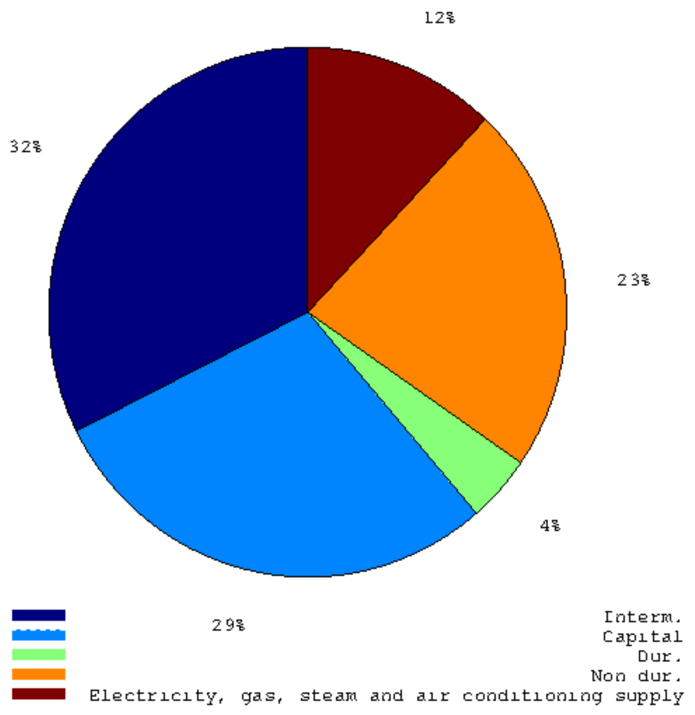
J 02 00033 g001
Figure 2. This pie graph shows the weights of main industry groupings in the Italian Industrial Production Index.
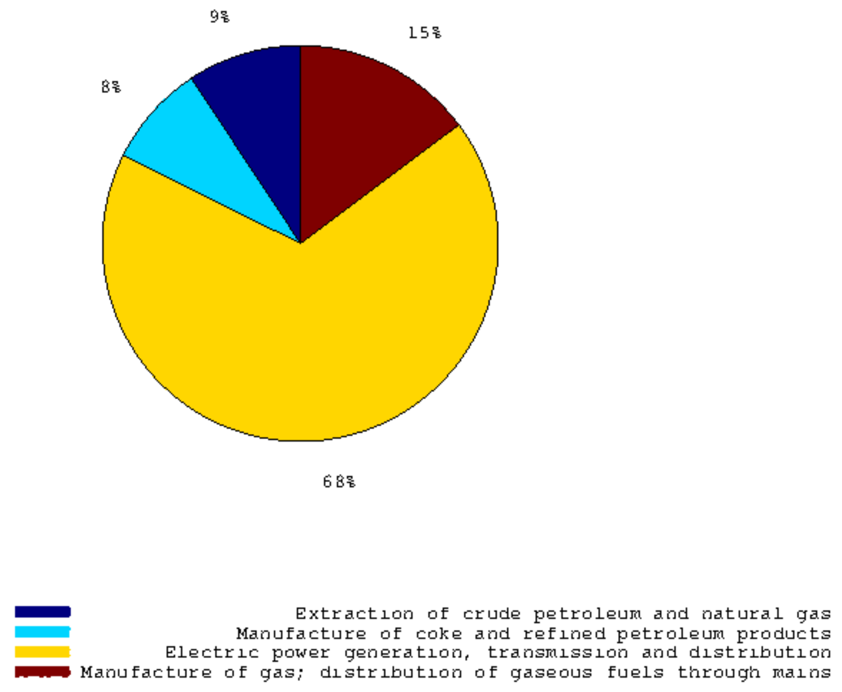
J 02 00033 g002
Figure 3. This pie graph shows the weights of every sub-component concerning the Italian Industrial Production Index of Electricity, gas, steam and air conditioning supply.
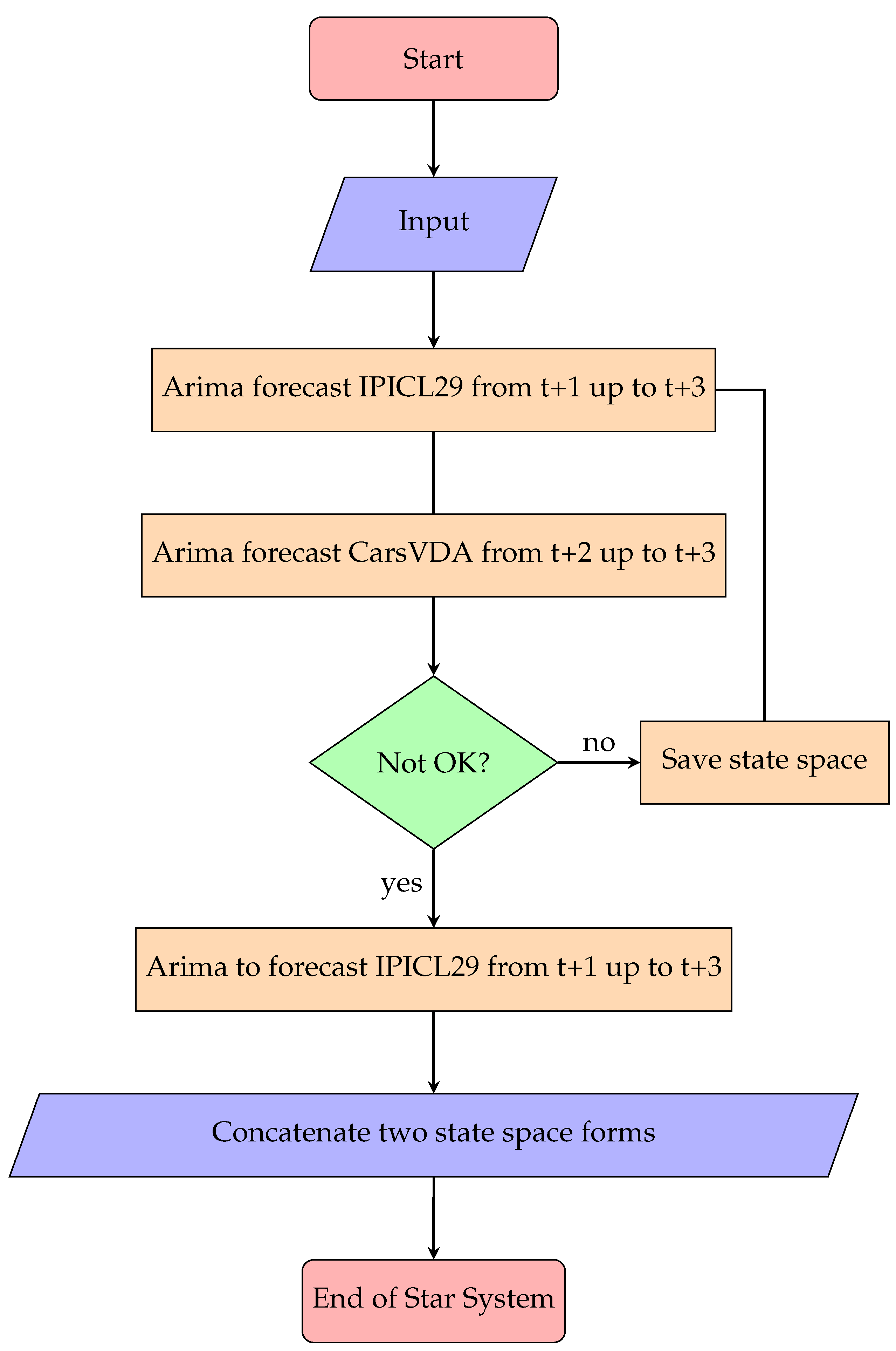
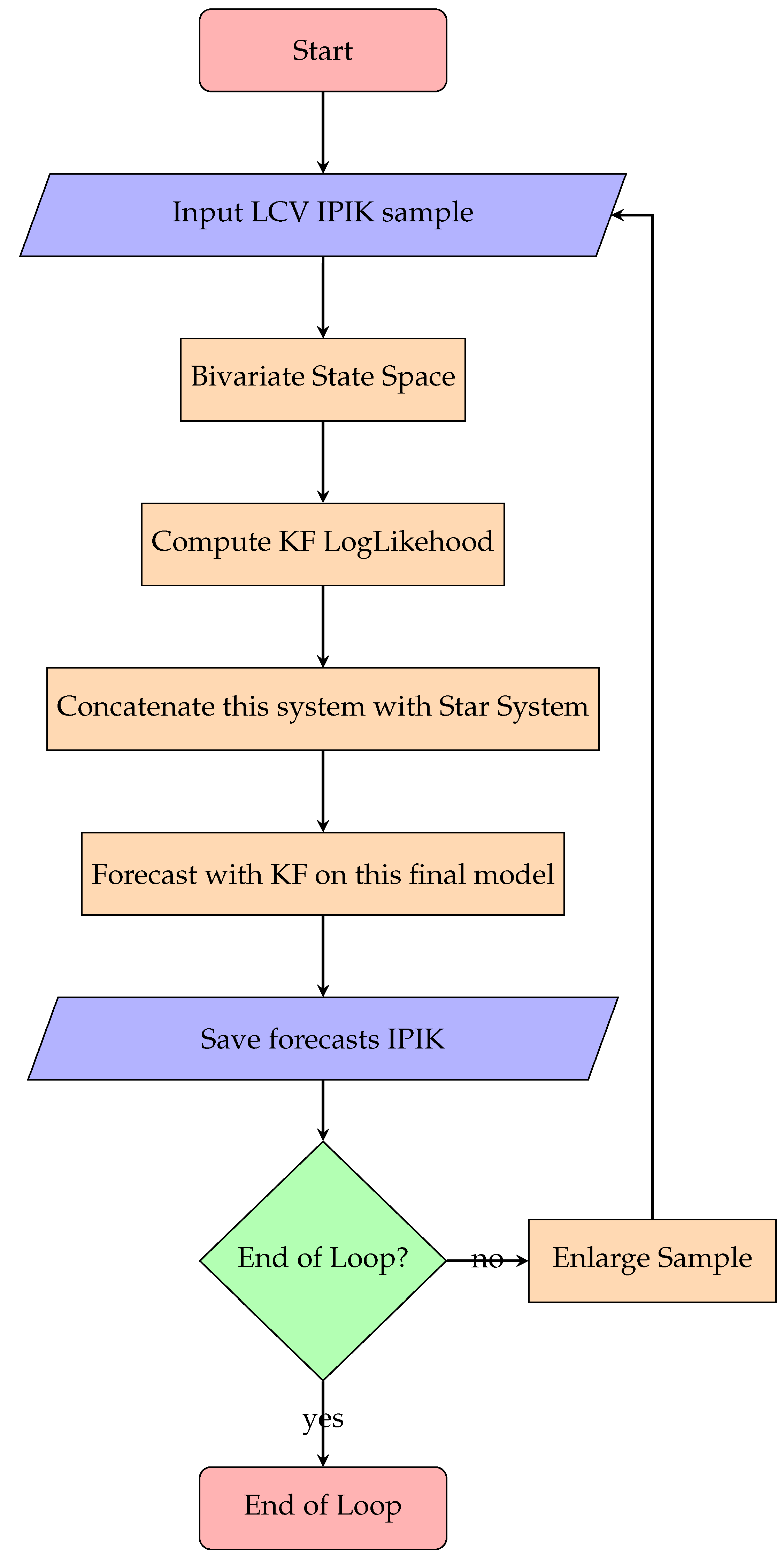
J 02 00033 g003
Figure 4. Star System.
J 02 00033 g004
Figure 5. Concatenate Seemingly Unrelated Time Series Equations with star system.
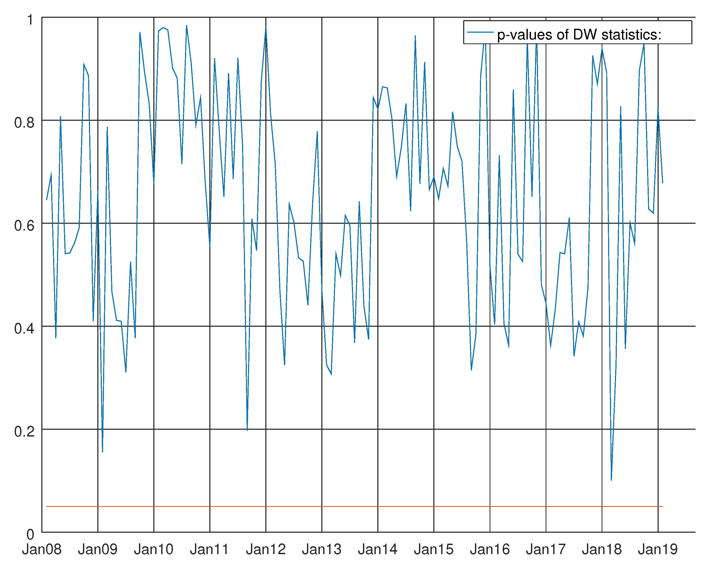
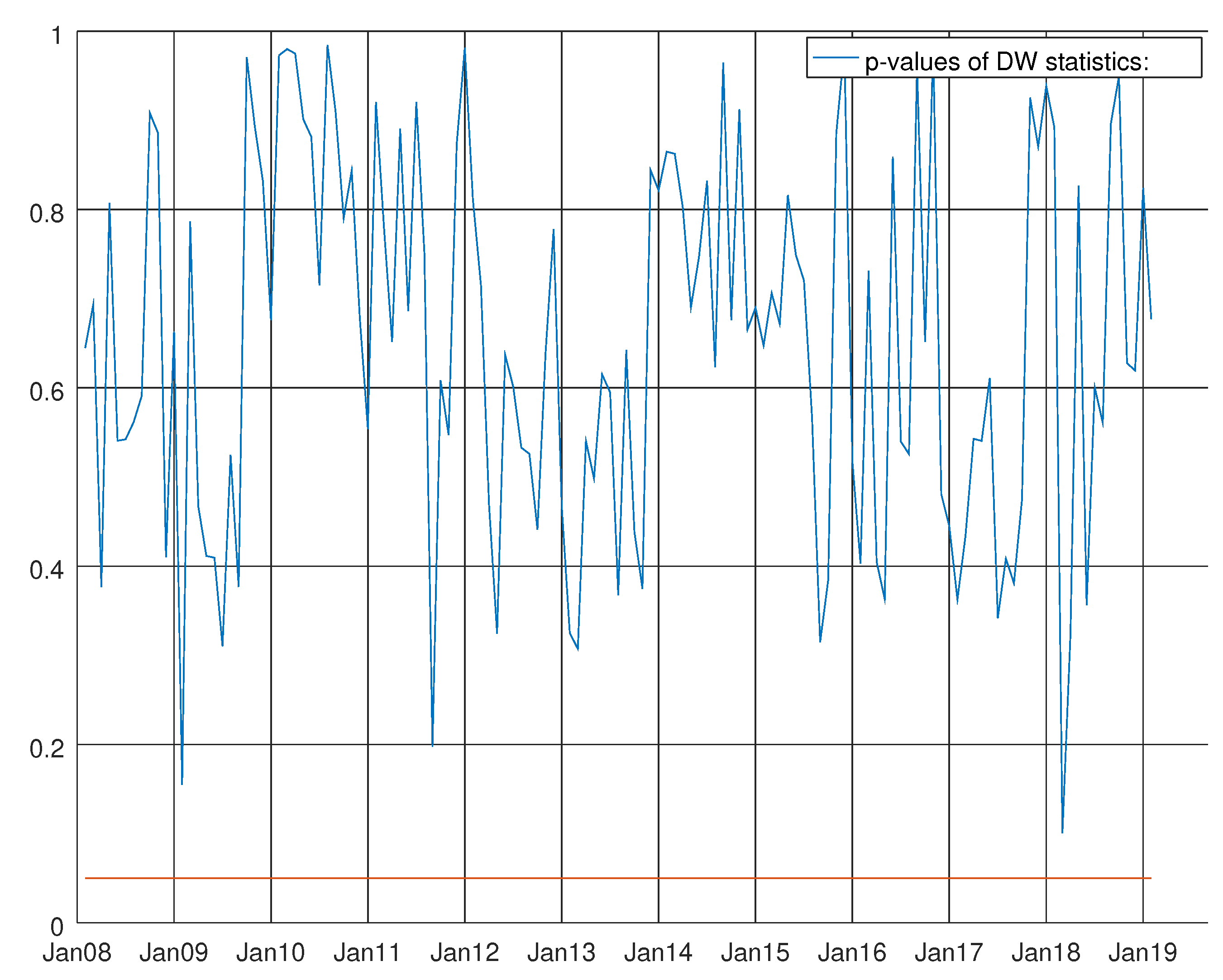
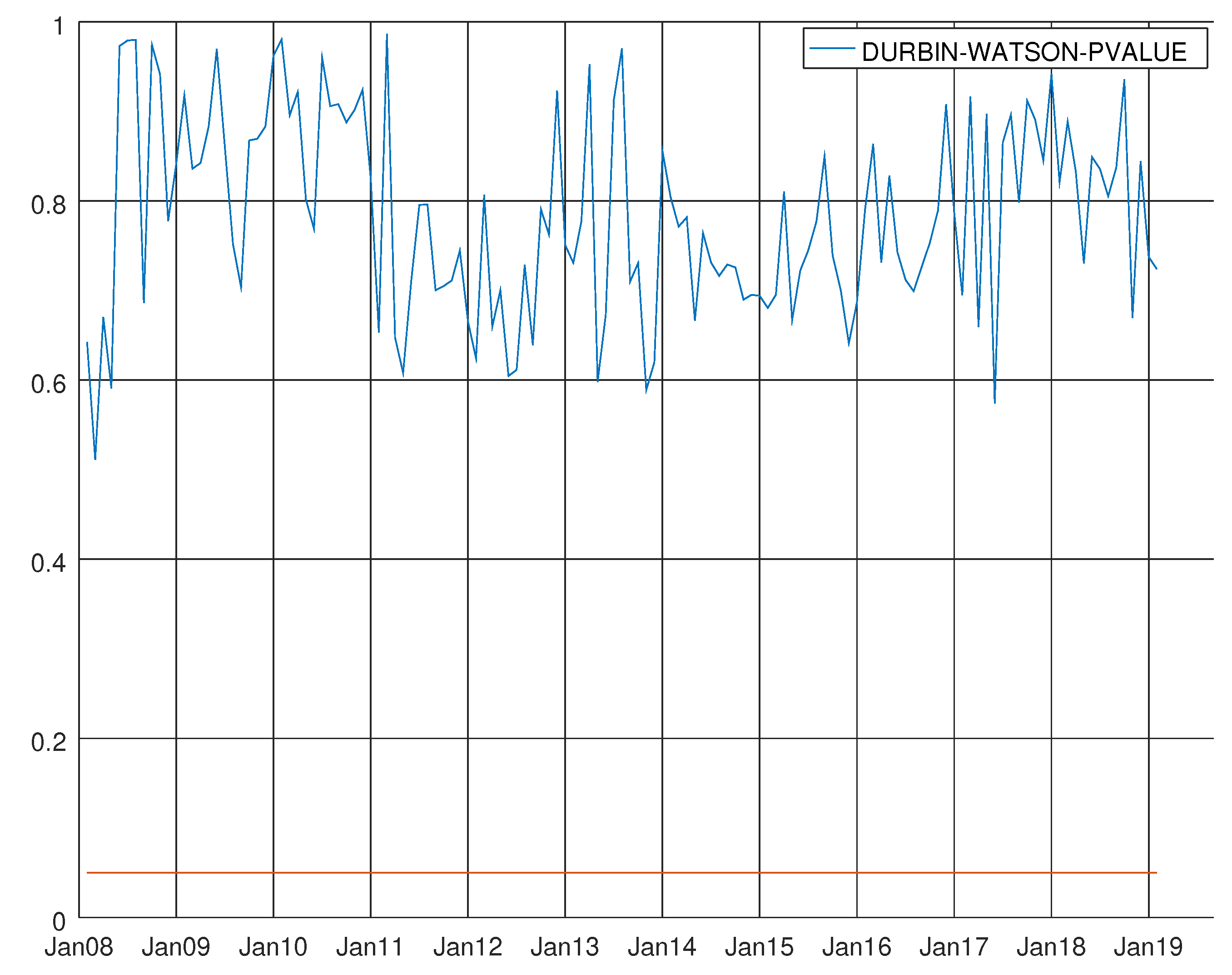
J 02 00033 g005
Figure 6. Graph showing the p-values of the Durbin–Watson test for the VARMA model using the hard data only. The null hypothesis states that residuals are not autocorrelated.
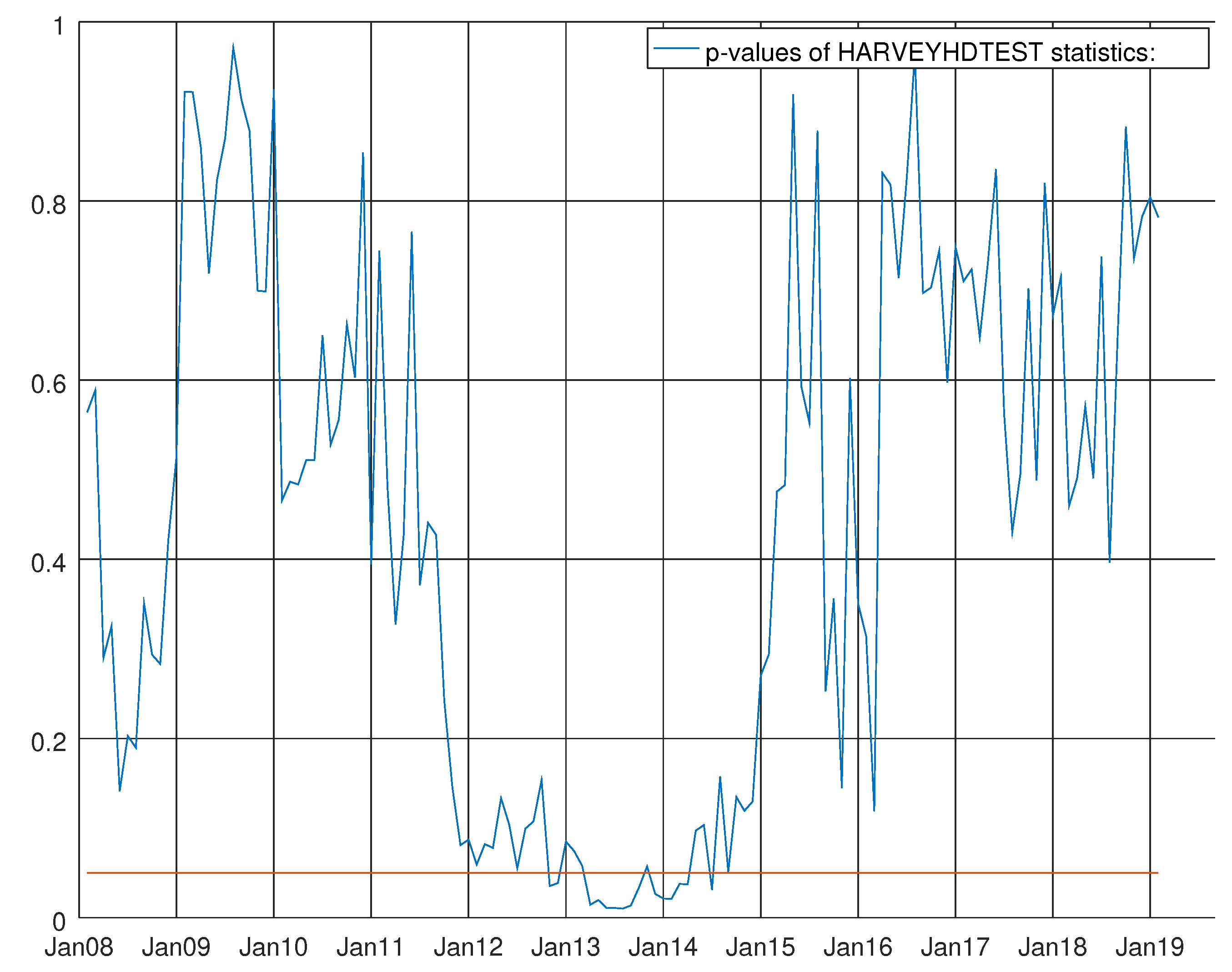
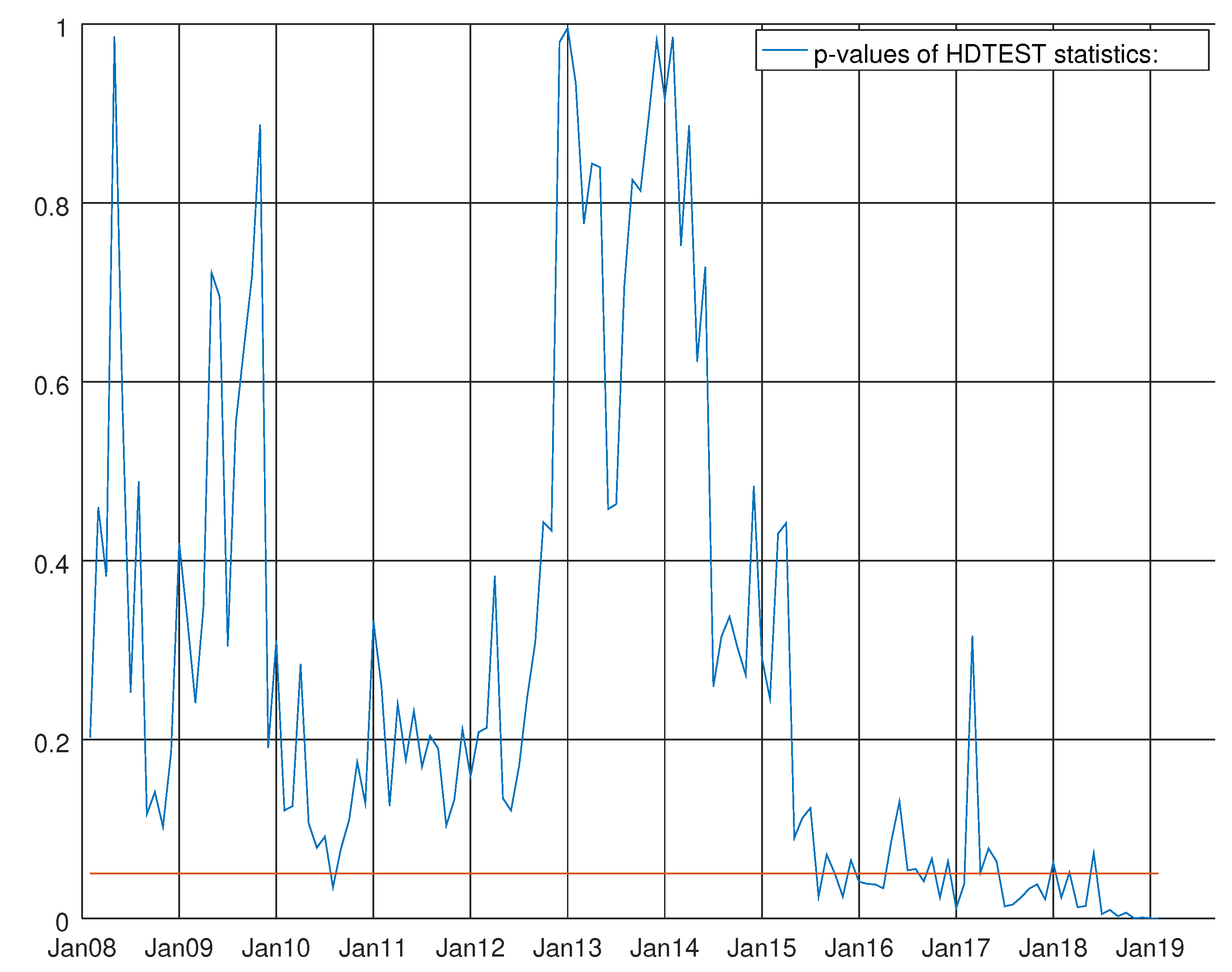
J 02 00033 g006
Figure 7. Graph showing the p-values of the Harvey heteroskedasticity test for the VARMA model using the hard data only. The null hypothesis states that the residuals are not heteroskedastic.
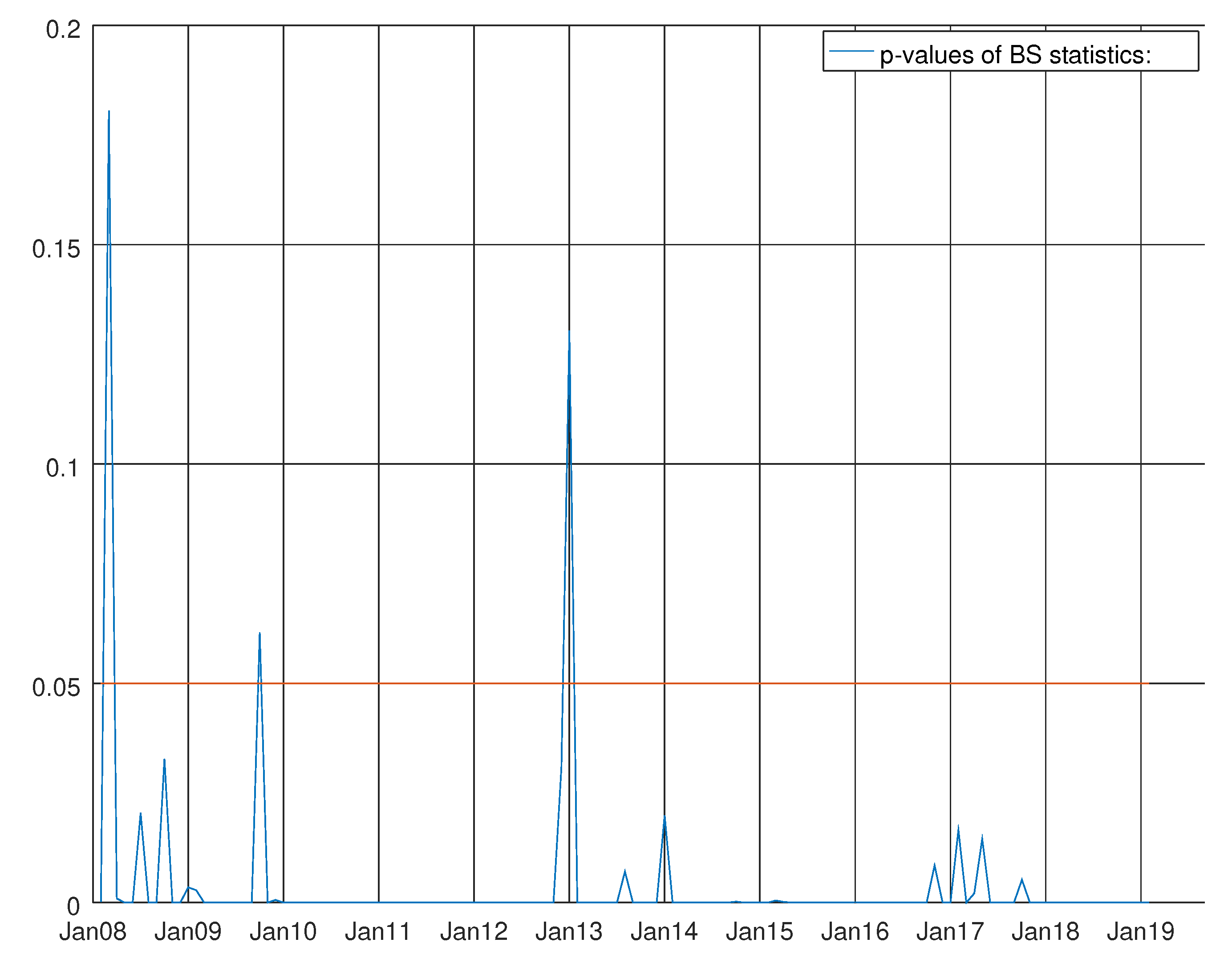
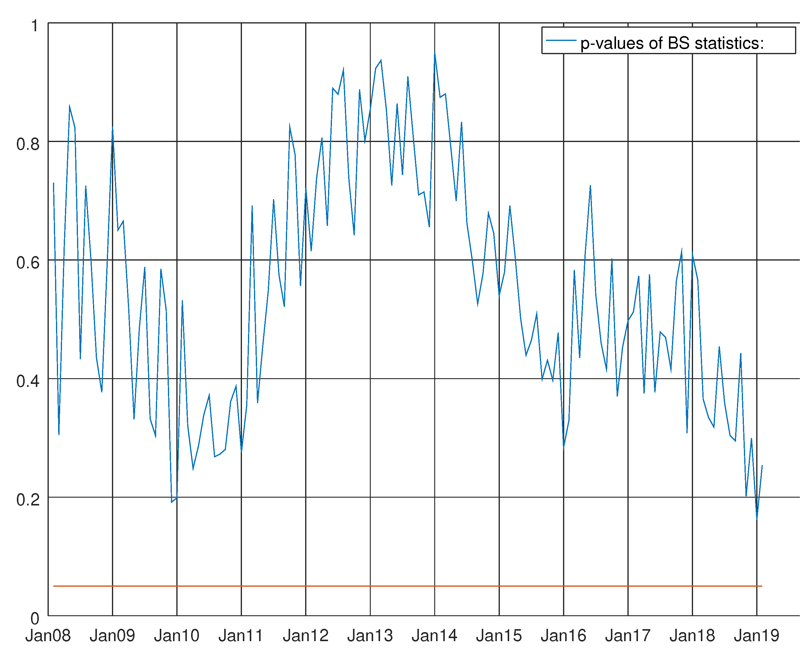
J 02 00033 g007
Figure 8. Graph showing the p-values of the Bowman–Shenton test for the VARMA model using the hard data only. The null hypothesis states that errors are normally distributed.
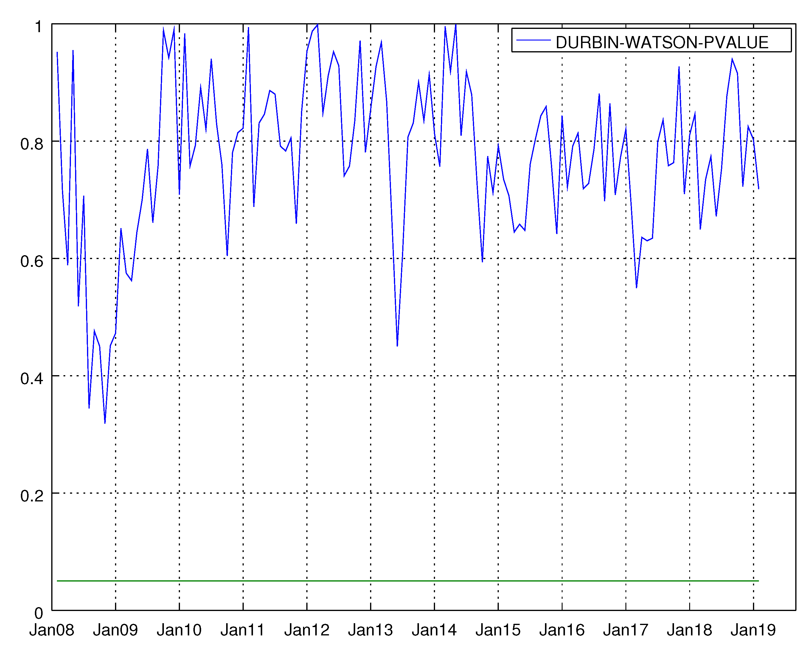
J 02 00033 g008
Figure 9. Graph showing the p-values of the Durbin–Watson test for the VARMA model using both hard and soft data for non-durable goods. The null hypothesis states that residuals are not autocorrelated.
J 02 00033 g009
Figure 10. Graph showing the p-values of the Bowman–Shenton test for the VARMA model using both hard and soft data for non-durable goods. The null hypothesis states that errors are normally distributed.
J 02 00033 g010
Figure 11. Graph showing the p-values of the Harvey heteroskedasticity test for the VARMA model using both hard and soft data for non-durable goods. The null hypothesis states that the residuals are not heteroskedastic.
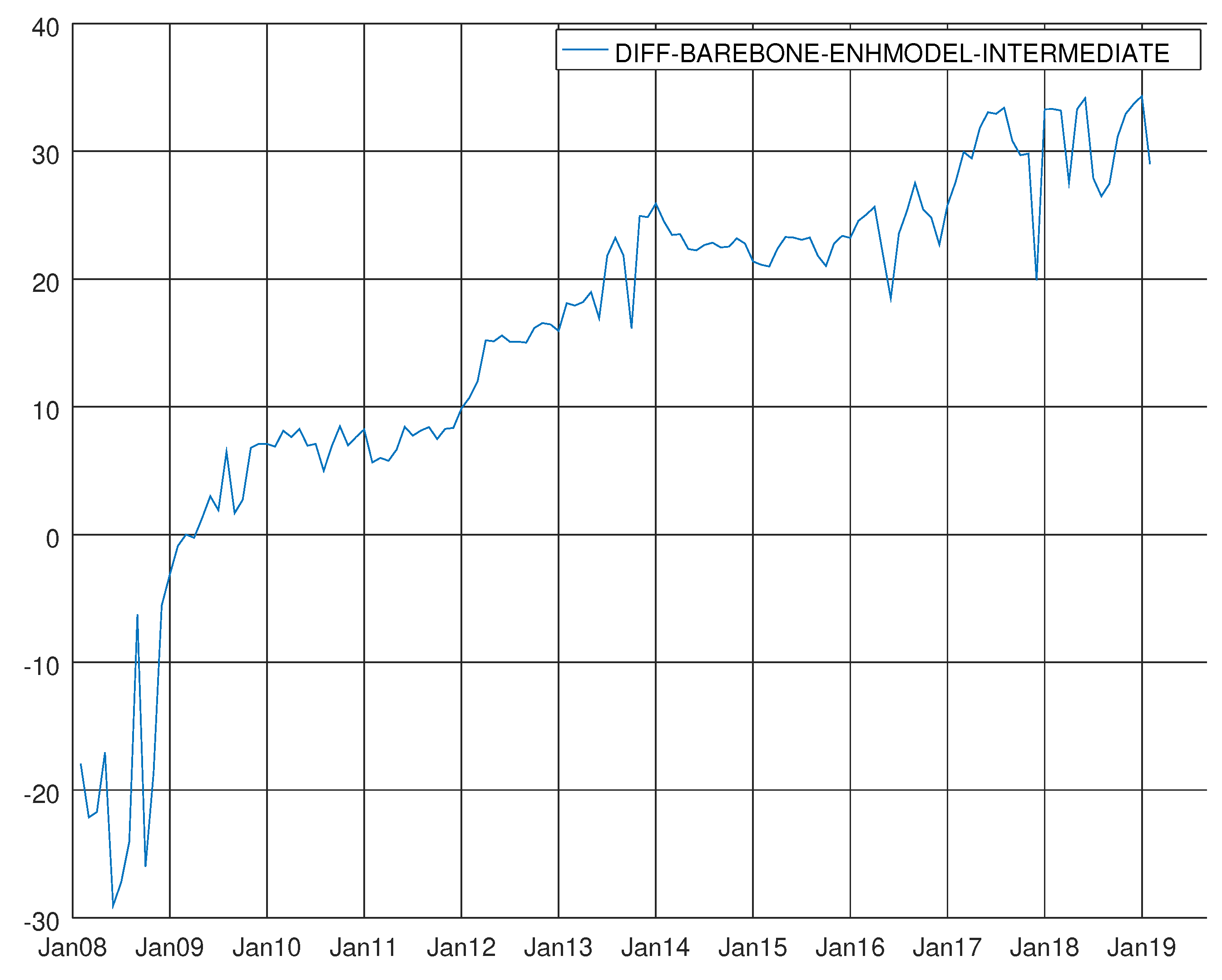
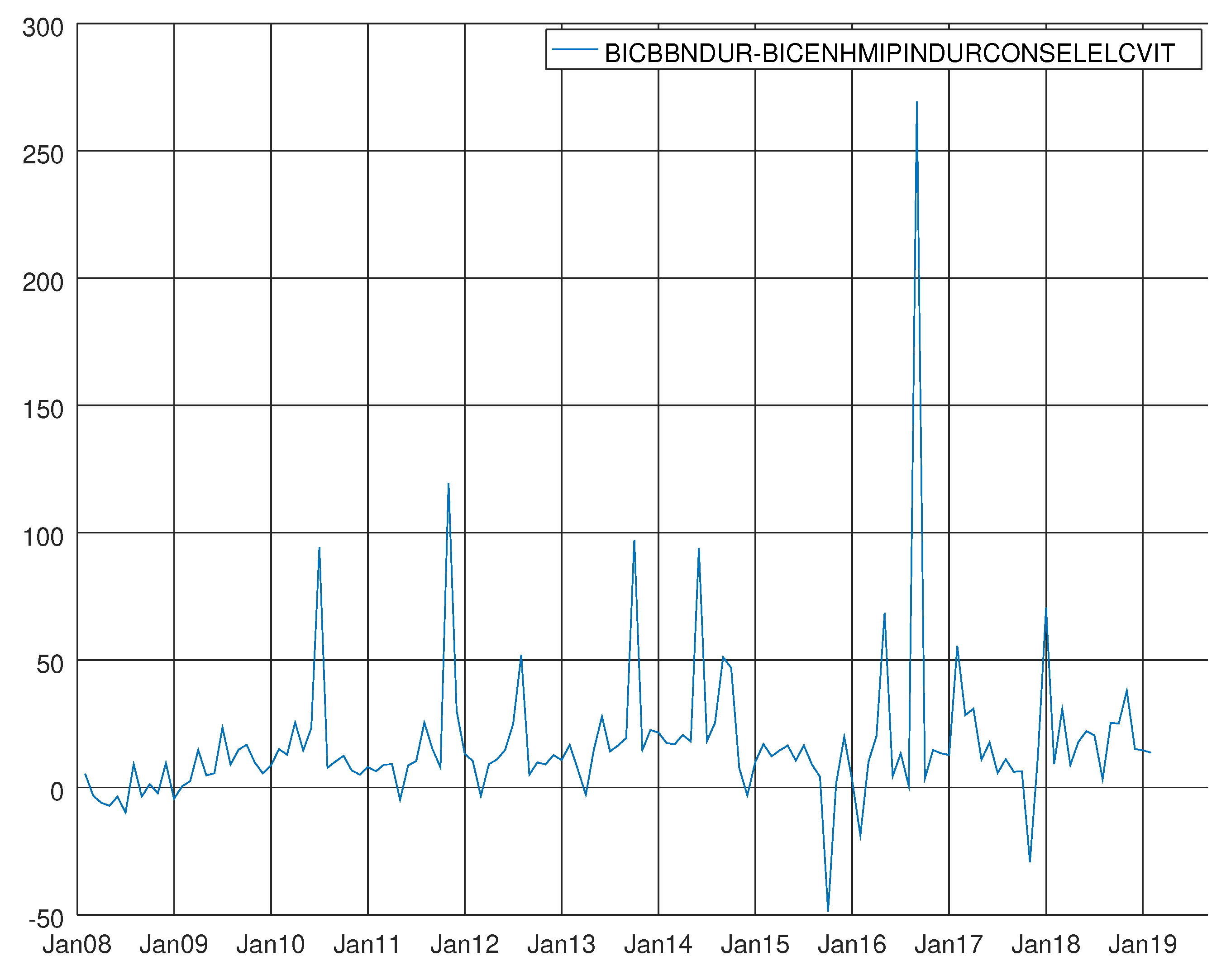
J 02 00033 g011
Figure 12. Graph showing the difference between the Bayesian information criterion of the barebone model and the enhanced model for intermediate goods. A negative value means that BB model prevails.
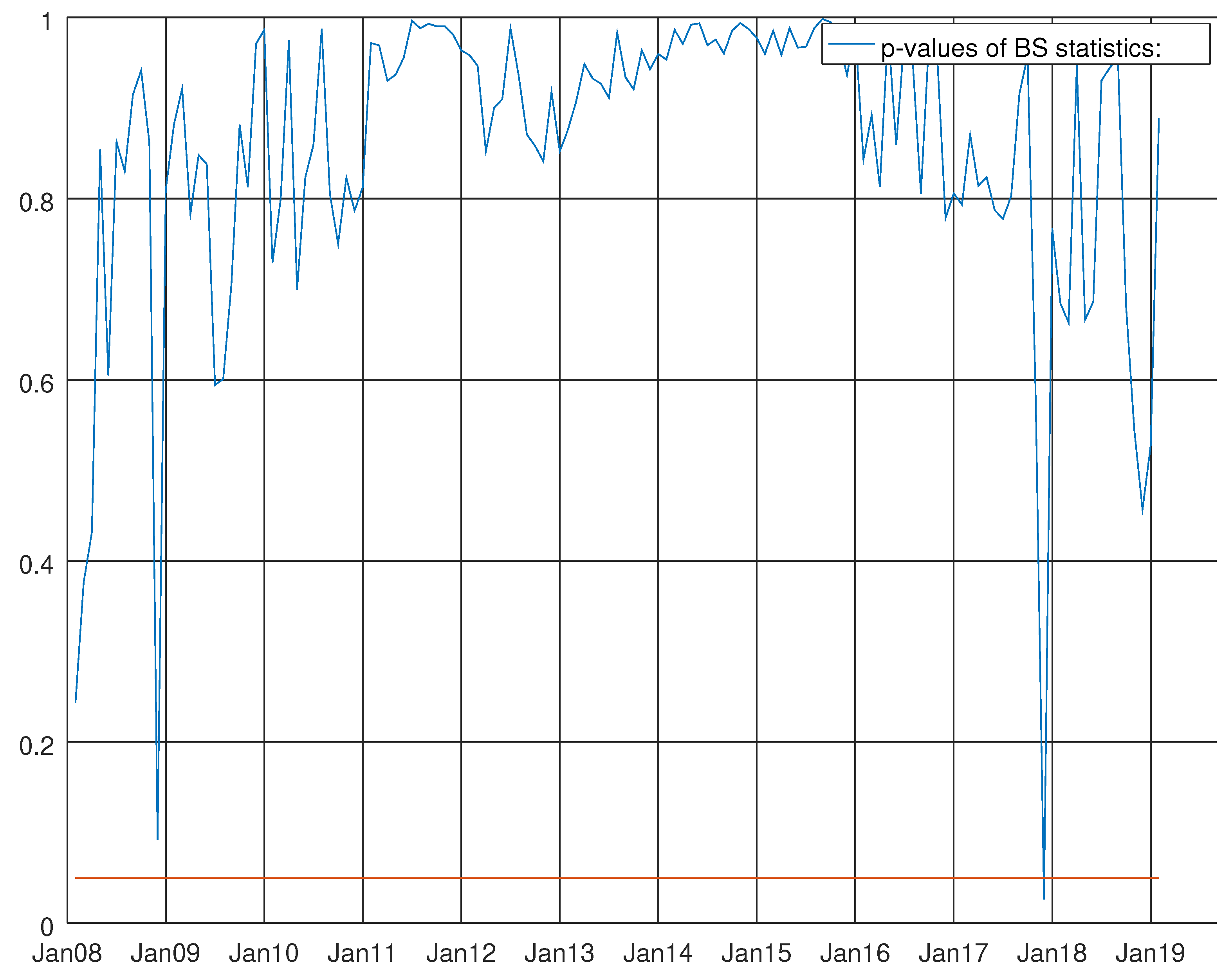
J 02 00033 g012
Figure 13. Graph showing the p-values of the Bowman–Shenton test for the enhanced model for intermediate goods. The null hypothesis states that errors are normally distributed.
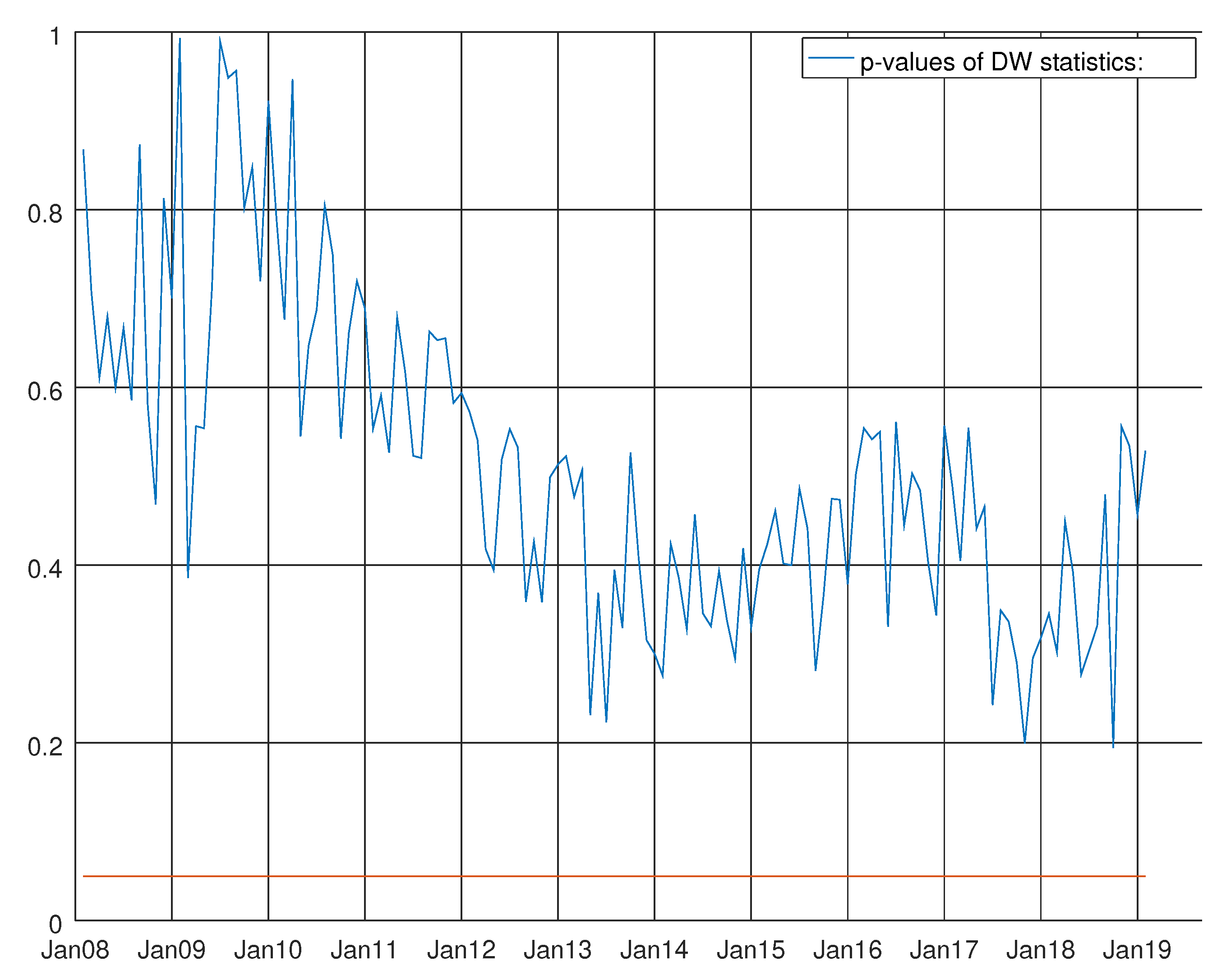
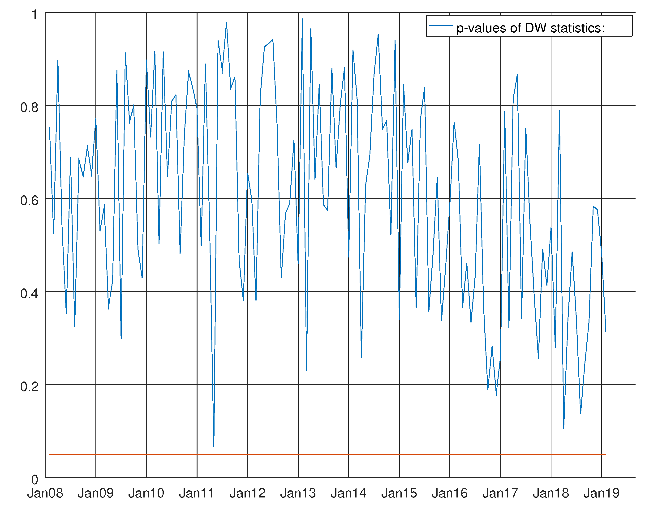
J 02 00033 g013
Figure 14. Graph showing the p-values of the Durbin–Watson test for the enhanced model for intermediate goods. The null hypothesis states that residuals are not autocorrelated.
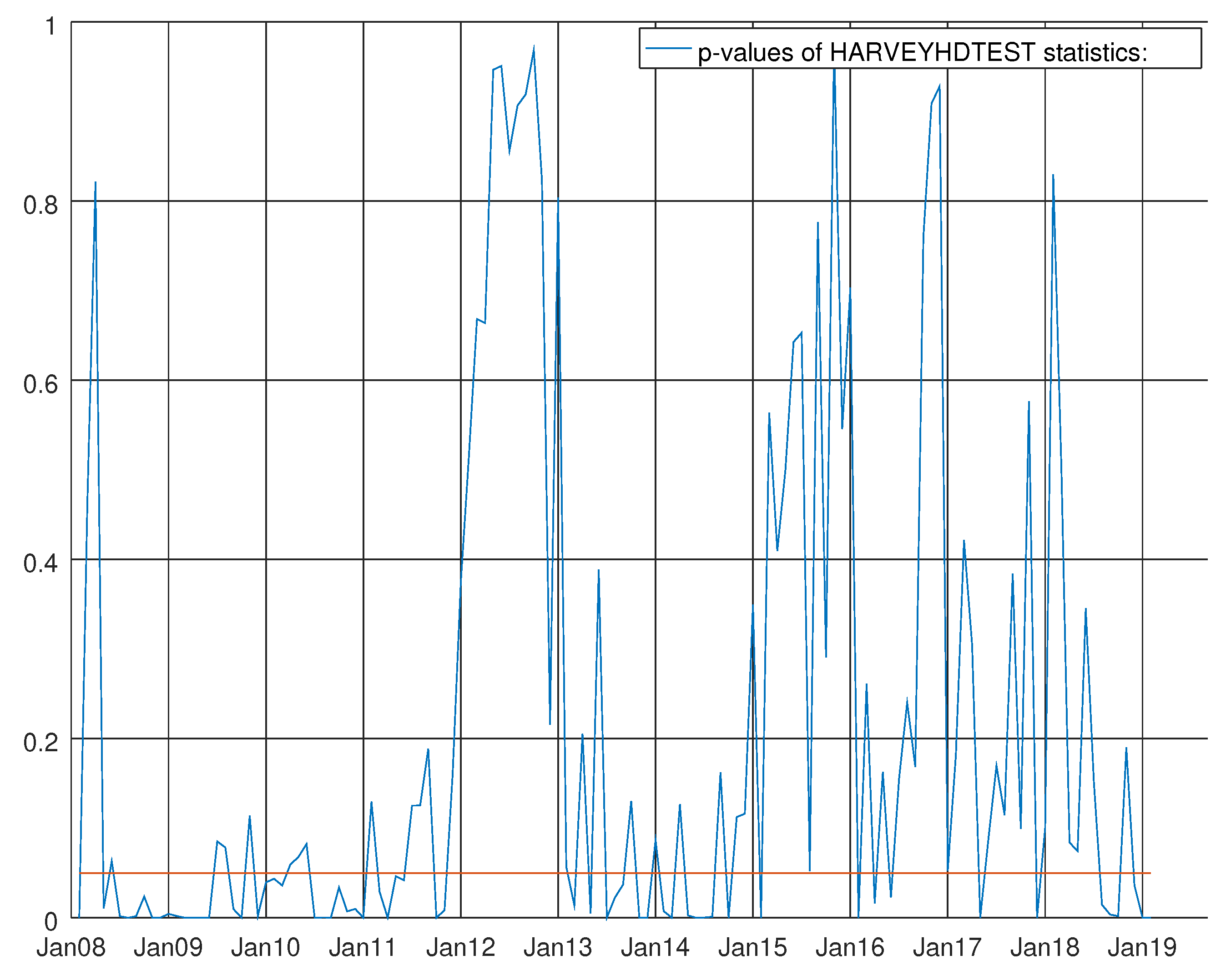
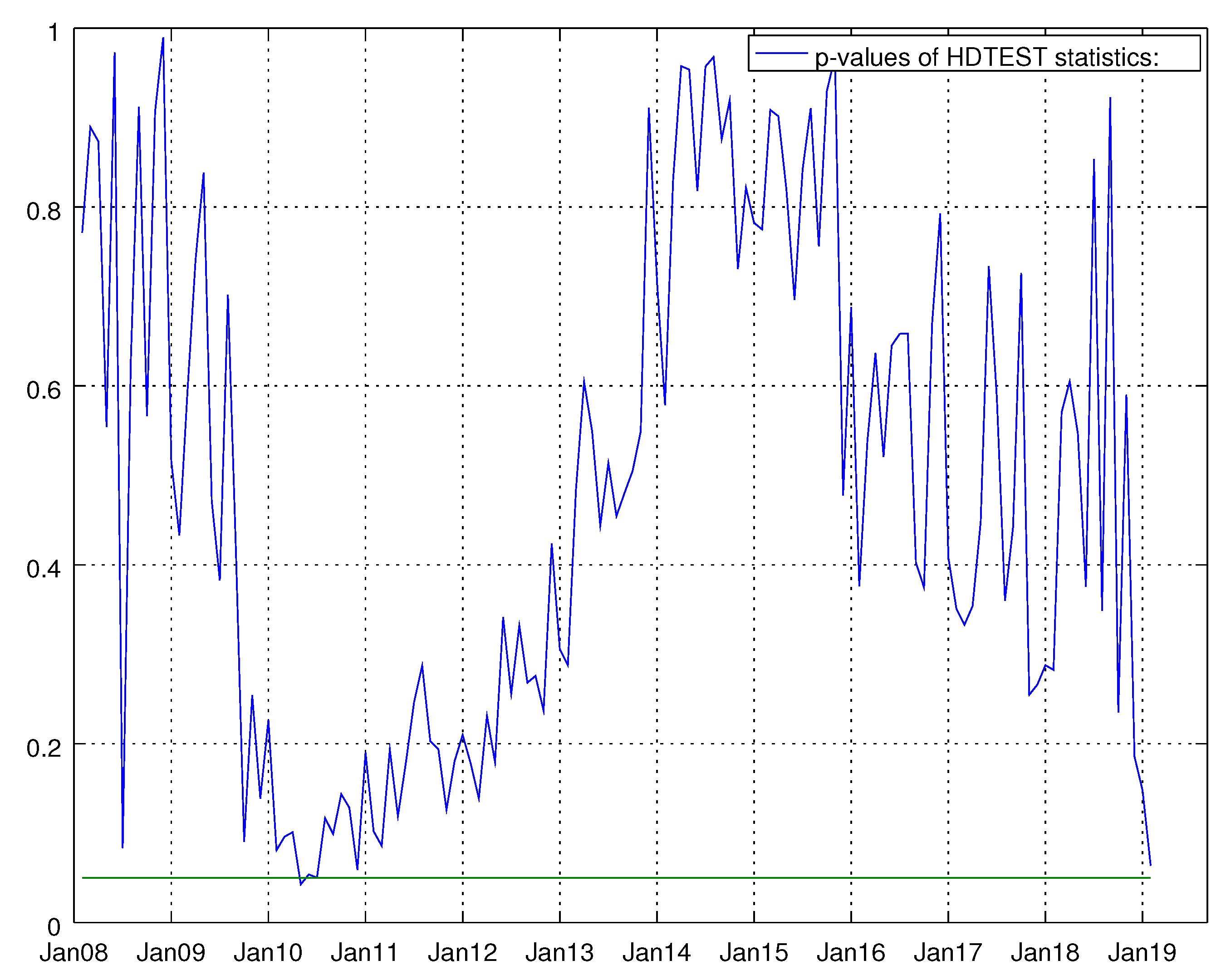
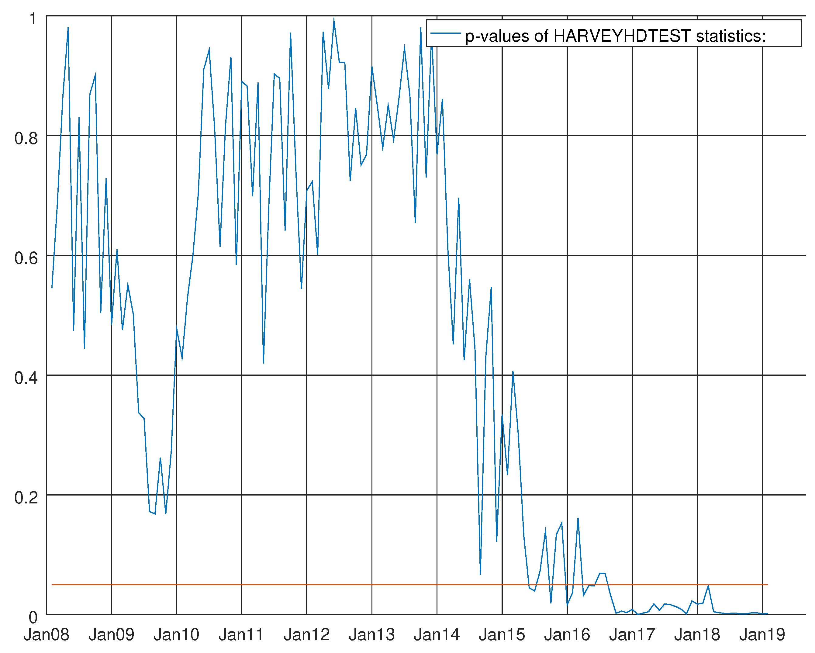
J 02 00033 g014
Figure 15. Graph showing the p-values of the Harvey heteroskedasticity test for the enhanced model for intermediate goods. The null hypothesis states that the residuals are not heteroskedastic.
J 02 00033 g015
Figure 16. Graph showing the difference between the Bayesian information criterion of the barebone model and the enhanced model for capital goods.
J 02 00033 g016
Figure 17. Graph showing the p-values of the Harvey heteroskedasticity test for the enhanced model for capital goods. The null hypothesis states that the residuals are not heteroskedastic.
J 02 00033 g017
Figure 18. Graph showing the p-values of the Bowman–Shenton test for the enhanced model for capital goods. The null hypothesis states that errors are normally distributed.
J 02 00033 g018
Figure 19. Graph showing the p-values of the Durbin–Watson test for the enhanced model for capital goods. The null hypothesis states that residuals are not autocorrelated.
J 02 00033 g019
Figure 20. Graph showing the p-values of the Durbin–Watson test for the barebone model for durable goods. The null hypothesis states that residuals are not autocorrelated.
J 02 00033 g020
Figure 21. Graph showing the p-values of the Bowman–Shenton test for the barebone model for durable goods. The null hypothesis states that errors are normally distributed.
J 02 00033 g021
Figure 22. Graph shows the p-values of the Harvey heteroskedasticity test for the barebone model for durable goods. The null hypothesis states that the residuals are not heteroskedastic.
J 02 00033 g022
Figure 23. Graph showing the difference between the Bayesian information criterion of the barebone model and the enhanced model for non-durable goods.
J 02 00033 g023
Figure 24. Graph showing the p-values of the Bowman–Shenton test for the enhanced model for non-durable goods. The null hypothesis states that errors are normally distributed.
J 02 00033 g024
Figure 25. Graph shows the p-values of the Durbin–Watson test for the enhanced model for non-durable goods. The null hypothesis states that residuals are not autocorrelated.
J 02 00033 g025
Figure 26. Graph showing the p-values of the Harvey heteroskedasticity test for the enhanced model for non-durable goods. The null hypothesis states that the residuals are not heteroskedastic.
J 02 00033 g026
Table 1. Information sources of data.
NameSeriesSourcesFreq.Time a
IPI5ISTATMonthly-
IPI of Electricity, gas, steam and air conditioning supply4ISTATMonthly-
GigaWatt Electricity net production1TERNAMonthly+20+25 days
GigaWatt Electricity Consumption1TERNAMonthly+35+40 days
GigaWatt Electricity Consumption1TERNADailyEvery Day
Total m3 of Compressed Natural Gas transported1SNAMDailyEvery Day
Production of m3 of Compressed Natural Gas1SNAMDailyEvery Day
M3 of Compressed Natural Gas for Thermoelectric use1SNAMDailyEvery Day
M3 of Compressed Natural Gas for Industrial use1SNAMDailyEvery Day
Registration of Light Commercial Vehicles in Italy1ACIMonthly+35+40 days
Registration of Light Commercial Vehicles in Spain1ANFACMonthly+35+40 days
Registration of Light Commercial Vehicles in France1CCFAMonthly+35+40 days
Registration of Light Commercial Vehicles in Germany1KBAMonthly+35+40 days
Truck Toll Mileage Index in Germany1DESTATISMonthly+35+40 days
IPI of Manufacture of motor vehicles, trailers and semi-trailers1ISTATMonthly-
Production of passengers cars in Germany1VDAMonthly+35+40 days
a Publication corresponds to amounts of days before the official release on ISTAT website.
Table 2. Information sources of data for VARMA using survey data.
NameSeriesSourcesFreq.Time a
IPI1ISTATMonthly-
GigaWatt Electricity Consumption1TERNAMonthly+35+40 days
Truck Toll Mileage Index in Germany1DESTATISMonthly+35+40 days
Climate Index (non-durable goods)1ISTATMonthly+35+40 days
General economy expectations (non-durable goods)1ISTATMonthly+35+40 days
Assessment of orders (non-durable goods)1ISTATMonthly+35+40 days
Assessment of domestic orders (non-durable goods)1ISTATMonthly+35+40 days
Assessment of export orders (non-durable goods)1ISTATMonthly+35+40 days
Production growth (non-durable goods)1ISTATMonthly+35+40 days
Assessment of stocks of finished products (non-durable goods)1ISTATMonthly+35+40 days
Orders expectations (non-durable goods)1ISTATMonthly+35+40 days
Production expectations (non-durable goods)1ISTATMonthly+35+40 days
Price expectations (non-durable goods)1ISTATMonthly+35+40 days
a Publication corresponds to amounts of days before the official release on ISTAT website.
Table 3. Comparison of mean absolute error and root mean squared error with expanding window applied to the VARMA using only hard data and both hard data and soft data, respectively (i.e., ISTAT survey), about the non-durable goods. The forecast windows expands itself from 2008:01 to 2018:12. The ratio between MAEs and RMSEs with respect to the benchmark are shown. A value less than one indicates an improvement over the benchmark.
Step 1Step 2Step 3
TYPE OF RATIOVARMAVARMAPLUSNDVARMAVARMAPLUSNDVARMAVARMAPLUSND
IMAE0.27490.63610.31420.91860.30890.8245
IMAE-20150.53161.06360.53561.56510.60341.4227
IRMSE0.23700.62280.27650.97920.26700.7521
IRMSE-20150.42681.06270.51101.65980.54471.4713
Table 4. Tests of equal predictive accuracy and test of forecast encompassing of VARMA using only hard data and both hard data and soft data, respectively (i.e., ISTAT survey), for non-durable goods. The forecast window expands itself from 2008:01 to 2018:12. The three tests are considered at the end of the sample and at the maximum value of forecast benchmark, i.e., August 2009. The p-values near to one show that the null hypothesis of equal predictive accuracy have been accepted with respect to the benchmark of Bulligan et al. For encompass test, the null hypothesis is that the forecast of the benchmark encompasses the forecast of the VARMA.
Step 1Step 2Step 3
MMDTEST-SUBSAMPLE-LOSS-FUNCTIONVARMAVARMAPLUSNDVARMAVARMAPLUSNDVARMAVARMAPLUSND
MMD-0801-1812-ABSERR0.92500.00370.71830.17880.50400.0621
MMD-0801-1812-ERR20.58500.00000.48870.23810.79130.0205
MMD-0801-0908-ABSERR0.77300.01490.31220.27030.68280.0795
MMD-0801-0908-ERR20.67700.03010.17230.78010.50700.0368
MMD-0801-0908-ENC0.43000.00170.42240.02580.02580.0082
MMD-0801-1812-ENC0.00000.00000.80110.39290.00210.0000
Table 5. Tests of equal predictive accuracy and test of forecast encompassing of VARMA using only hard data and both hard data and soft data, respectively, (i.e., ISTAT survey) for non-durable goods. The forecast windows expands itself from 2008:01 to 2018:12. The three tests are considered at the end of the sample and at the maximum value of forecast benchmark, i.e., August 2009. The p-values near one show that null hypothesis of equal predictive accuracy between the VARMA that uses only hard data and the VARMA that uses hard data plus soft data for non-durable goods has been accepted. For encompass test, the null hypothesis is that the forecast of the VARMA using only hard data encompasses the forecast of the VARMA using only hard data and soft data for non-durable goods.
Step 1Step 2Step 3
MMDTEST-SUBSAMPLE-LOSS-FUNCTIONVARMA vs. VARMAPLUSNDVARMA vs. VARMAPLUSNDVARMA vs. VARMAPLUSND
MMD-0801-1812-ABSERR0.00130.276610.1283
MMD-0801-1812-ERR20.00460.28890.0281
MMD-0801-0908-ABSERR0.02380.19810.0800
MMD-0801-0908-ERR20.03490.49560.0548
MMD-0801-0908-ENC0.00180.01730.0120
MMD-0801-1812-ENC0.00000.80610.0000
Table 6. Model confidence set hierarchy loss function is the absolute error at the end of the sample for intermediate goods model comparison α = 0 . 05 , number of bootstrap replications = 5000 and block length = 12. The null hypothesis is that the average performance of the model in the row is as small as the minimum average performance across the remaining models. The alternative is that the minimum average loss across the remaining models is smaller than the average performance of the model in the row.
IndexStep 1Step 2Step 3
IPI-BEN-INTERM0.02160.01020.0088
BBLCVDE0.03620.36340.7236
BBLCVFR0.03620.36340.8332
BBLCVSP0.21840.36340.8332
BBTTMI0.21840.59040.8332
ENHTTMI1.00001.00001.0000
Table 7. Comparison of the ratios of mean absolute error for models for intermediate goods with an expanding window from 2008:01 to 2018:12.
IndexStep 1Step 2Step 3
BBLCVDE0.47490.52840.5672
BBLCVFR0.45350.51810.5537
BBLCVSP0.44310.51800.5478
BBTTMI0.43040.51340.5560
ENHTTMI0.43450.48850.5362
Table 8. Model confidence set hierarchy loss function is the squared error at the end of the sample for intermediate goods model comparison α = 0 . 05 , number of bootstrap replications = 5000 and block length = 12. The null hypothesis is that the average performance of the model in the row is as small as the minimum average performance across the remaining models. The alternative is that the minimum average loss across the remaining models is smaller than the average performance of the model in the row.
IndexStep 1Step 2Step 3
IPI-BEN-INTERM0.14900.15300.1414
BBLCVDE0.14900.15300.1414
BBLCVFR0.14900.27980.3096
BBLCVSP0.35680.27980.3096
BBTTMI0.35680.27980.3096
ENHTTMI1.00001.00001.0000
Table 9. Comparison of the ratios of RMSE for models for intermediate goods with an expanding window from 2008:01 to 2018:12.
IndexStep 1Step 2Step 3
BBLCVDE0.66030.74190.7993
BBLCVFR0.61430.71660.7496
BBLCVSP0.58350.66980.7009
BBTTMI0.63230.73440.7774
ENHTTMI0.62960.65390.7011
Table 10. Model confidence set hierarchy loss function is the absolute error at the end of the sample for capital goods model comparison α = 0 . 05 , number of bootstrap replications = 5000 and block length = 12. The null hypothesis is that the average performance of the model in the row is as small as the minimum average performance across the remaining models. The alternative is that the minimum average loss across the remaining models is smaller than the average performance of the model in the row.
IndexStep 1Step 2Step 3
IPI-BEN-CAPITAL0.00400.00360.0010
BBLCVDE0.66180.03560.3012
BBLCVFR0.82220.91660.9820
BBLCVSP0.99520.93280.9820
BBTMI0.99520.93280.9820
ENHTTMI1.00001.00001.0000
Table 11. Comparison of the ratios of absolute error for models for capital goods with an expanding window from 2008:01 to 2018:12.
IndexStep 1Step 2Step 3
BBLCVDE0.45080.49430.5391
BBLCVFR0.45430.48460.5327
BBLCVSP0.43630.49240.5386
BBTTMI0.43310.49070.5355
ENHTTMI0.43440.53810.5755
Table 12. Comparison of the ratios of RMSE for models for capital goods with an expanding window from 2008:01 to 2018:12.
IndexStep 1Step 2Step 3
BBLCVDE0.52870.57950.6065
BBLCVFR0.53930.56900.5911
BBLCVSP0.46060.57050.5558
BBTTMI0.53500.59350.6137
ENHTTMI0.52920.62610.6586
Table 13. Model Confidence Set Hierarchy Loss function is the squared error at the end of the sample for capital goods model comparison α = 0 . 05 , number of bootstrap replications = 5000 and block length = 12. The null hypothesis is that the average performance of the model in the row is as small as the minimum average performance across the remaining models. The alternative is that the minimum average loss across the remaining models is smaller than the average performance of the model in the row.
IndexStep 1Step 2Step 3
IPI-BEN-CAPITAL0.14120.07700.0708
BBLCVDE0.71240.07700.0708
BBLCVFR0.71240.70620.6688
BBLCVSP0.71240.77360.6688
BBTMI0.71240.88820.6688
ENHTTMI1.00001.00001.0000
Table 14. Model confidence set hierarchy loss function is the absolute error at the end of the sample for non-durable goods model comparison α = 0 . 05 , number of bootstrap replications = 5000 and block length = 12. The null hypothesis is that the average performance of the model in the row is as small as the minimum average performance across the remaining models. The alternative is that the minimum average loss across the remaining models is smaller than the performance of the model in the row.
IndexStep 1Step 2Step 3
IPI-BEN-NDUR0.00000.00000.0000
BBSNAMINDUSTRIAL0.00000.00000.0002
ENHSNAMINDUSTRIAL1.00001.00001.0000
Table 15. Model confidence set hierarchy loss function is the squared error at the end of the sample for non-durable goods model comparison α = 0 . 05 , number of bootstrap replications = 5000 and block length = 12. The null hypothesis is that the average performance of the model in the row is as small as the minimum average performance across the remaining models. The alternative is that the minimum average loss across the remaining models is smaller than the average performance of the model in the row.
IndexStep 1Step 2Step 3
IPI-BEN-NDUR0.00000.00000.0000
BBSNAMINDUSTRIAL0.00000.00000.0002
ENHSNAMINDUSTRIAL1.00001.00001.0000
Table 16. Comparison of the ratios of absolute error for models for capital goods with an expanding window from 2008:01 to 2018:12.
IndexStep 1Step 2Step 3
IPI-BEN-NDUR1.00001.00001.0000
BBSNAMINDUSTRIAL0.65130.74340.7251
ENHSNAMINDUSTRIAL0.64070.57870.5964
Table 17. Comparison of the ratios of RMSE for models for capital goods with an expanding window from 2008:01 to 2018:12.
IndexStep 1Step 2Step 3
IPI-BEN-NDUR1.00001.00001.0000
BBSNAMINDUSTRIAL0.62920.73340.7211
ENHSNAMINDUSTRIAL0.62860.69690.7053
Table 18. Comparison of the ratios of mean absolute error with an expanding window from 2008:01 to 2018:12.
IndexStep 1Step 2Step 3
IPI-INT0.43450.48850.5362
IPI-CAP0.42000.52650.5692
IPI-DUR0.49760.50060.5088
IPI-NDUR0.64070.71960.7329
IPI-ENERGY0.14980.51450.5328
IPI-AGG0.35030.42540.4611
IPI-BENAGG1.00191.00441.0035
Table 19. Modified Diebold–Mariano statistics for equality of forecast accuracy of two forecasts under general assumptions with an expanding window from 2008:01 to 2018:12. The null hypothesis is that the two methods have the same forecast accuracy. The loss function is the absolute error.
IndexStep 1Step 2Step 3
IPI-INT0.00000.00000.0000
IPI-CAP0.00000.00000.0000
IPI-DUR0.04520.05390.0516
IPI-NDUR0.00000.00000.0000
IPI-ENERGY0.00000.00000.0000
IPI-AGG0.00000.00000.0000
Table 20. Comparison of the ratio between mean absolute errors with an expanding window from 2015:01 to 2018:12.
IndexStep 1Step 2Step 3
IPI-INT0.43730.59350.6499
IPI-CAP0.38900.44120.4288
IPI-DUR0.86890.90720.8852
IPI-NDUR0.59740.66730.7049
IPI-ENERGY0.16030.60200.6094
IPI-AGG0.35900.52060.4957
IPI-BENAGG1.00511.01801.0170
Table 21. Modified Diebold–Mariano statistics for the equality of forecast accuracy of two forecasts under general assumptions with an expanding window from 2015:01 to 2018:12. The null hypothesis is that the two methods have the same forecast accuracy. The Loss function is the absolute error.
IndexStep 1Step 2Step 3
IPI-INT0.00010.00570.0179
IPI-CAP0.00000.00000.0000
IPI-DUR0.34690.49860.4446
IPI-NDUR0.00000.00000.0000
IPI-ENERGY0.00000.00810.0012
IPI-AGG0.00000.00010.0002
Table 22. Comparison between RMSE ratios with an expanding window from 2008:01 to 2018:12.
IndexStep 1Step 2Step 3
IPI-INT0.62960.65390.7011
IPI-CAP0.56310.66950.7140
IPI-DUR0.92980.91360.8500
IPI-NDUR0.62860.69690.7053
IPI-ENERGY0.15560.53610.5550
IPI-AGG0.39170.47240.5249
IPI-BENAGG0.99821.00361.0037
Table 23. Modified Diebold–Mariano statistics for the equality of forecast accuracy of two forecasts under general assumptions with an expanding window from 2008:01 to 2018:12. The null hypothesis is that the two methods have the same forecast accuracy. The loss function is the squared error.
IndexStep 1Step 2Step 3
IPI-INT0.03890.02910.0338
IPI-CAP0.00410.02680.0252
IPI-DUR0.79850.80100.9780
IPI-NDUR0.00000.00000.0000
IPI-ENERGY0.00000.00000.0000
IPI-AGG0.00000.00000.0000
Table 24. Comparison of mean ratio between RMSEs with an expanding window from 2015:01 to 2018:12.
IndexStep 1Step 2Step 3
IPI-INT0.45170.63240.6783
IPI-CAP0.40660.43570.4306
IPI-DUR1.40711.47481.4073
IPI-NDUR0.58910.63920.6439
IPI-ENERGY0.15580.59210.6161
IPI-AGG0.36420.51760.4926
IPI-BENAGG0.99771.00481.0006
Table 25. Modified Diebold–Mariano statistics for the equality of forecast accuracy of two forecasts under general assumptions with an expanding window from 2015:01 to 2018:12. The null hypothesis is that the two methods have the same forecast accuracy. The loss function is the squared error.
IndexStep 1Step 2Step 3
IPI-INT0.00000.00030.0005
IPI-CAP0.00030.01460.0312
IPI-DUR0.00010.00010.0001
IPI-NDUR0.86940.79450.9430
IPI-ENERGY0.00000.00000.0000
IPI-AGG0.00020.01210.0053
Table 26. Comparison of ratios between mean absolute errors with an expanding window for electricity from 2008:01 to 2018:12.
IndexStep 1Step 2Step 3
IPI-EXTRA0.39100.40730.7706
IPI-PETROL0.61500.67120.7422
IPI-PRODELE0.00750.56860.6056
IPI-CNG0.15430.20730.7581
IPI-AGG0.14980.51450.5328
IPI-BENAGG0.99390.98300.9836
Table 27. Modified Diebold–Mariano statistics for the equality of forecast accuracy of two forecasts under general assumptions with expanding window from 2008:01 to 2018:12. The null hypothesis is that the two methods have the same forecast accuracy. The loss function is the absolute error.
IndexStep 1Step 2Step 3
IPI-EXTRA0.00000.00000.0094
IPI-PETROL0.00000.00000.0000
IPI-PRODELE0.00000.00050.0000
IPI-CNG0.00000.00000.0004
IPI-AGG0.00000.00000.0000
Table 28. Comparison of the ratio between mean absolute errors with an expanding window for electricity from 2015:01 to 2018:12.
IndexStep 1Step 2Step 3
IPI-EXTRA0.37070.38930.6791
IPI-PETROL0.67630.79530.7441
IPI-PRODELE0.00540.67130.7433
IPI-CNG0.09610.15930.7501
IPI-AGG0.16030.60200.6094
IPI-BENAGG0.87330.85730.8575
Table 29. Modified Diebold–Mariano for the equality of forecast accuracy of two forecasts under general assumptions with an expanding window from 2015:01 to 2018:12. The null hypothesis is that the two methods have the same forecast accuracy. The loss function is the absolute error.
IndexStep 1Step 2Step 3
IPI-EXTRA0.000000.000000.02050
IPI-PETROL0.009500.062200.20580
IPI-PRODELE0.000000.785300.03960
IPI-CNG0.000000.000000.02340
IPI-AGG0.000000.008100.00120
Table 30. Comparison of the ratio between RMSEs with an expanding window for electricity from 2008:01 to 2018:12.
IndexStep 1Step 2Step 3
IPI-EXTRA0.38520.39670.8318
IPI-PETROL0.62720.70610.7946
IPI-PRODELE0.01000.44960.4778
IPI-CNG0.01840.02350.0815
IPI-AGG0.15560.53610.5550
IPI-BENAGG1.00120.99860.9992
Table 31. Modified Diebold–Mariano statistics for the equality of forecast accuracy of two forecasts under general assumptions with an expanding window from 2008:01 to 2018:12. The null hypothesis is that the two methods have the same forecast accuracy. The loss function is the squared error.
IndexStep 1Step 2Step 3
IPI-EXTRA0.00000.00000.1298
IPI-PETROL0.00000.00000.0001
IPI-PRODELE0.00000.00100.0000
IPI-CNG0.00000.00000.0003
IPI-AGG0.00000.00000.0000
Table 32. Comparison of the ratio between RMSEs with an expanding window for electricity from 2015:01 to 2018:12.
IndexStep 1Step 2Step 3
IPI-EXTRA0.33300.35240.6130
IPI-PETROL0.72240.75410.7532
IPI-PRODELE0.00720.46590.5101
IPI-CNG0.01050.01800.0787
IPI-AGG0.15580.59210.6161
IPI-BENAGG0.91290.90190.8997
Table 33. Modified Diebold–Mariano statistics for the equality of forecast accuracy of two forecasts under general assumptions with an expanding window from 2015:01 to 2018:12. The null hypothesis is that the two methods have the same forecast accuracy. The loss function is the squared error.
IndexStep 1Step 2Step 3
IPI-EXTRA0.00220.00230.0164
IPI-PETROL0.02120.15710.4489
IPI-PRODELE0.00170.56290.0809
IPI-CNG0.00000.00000.0163
IPI-AGG0.00020.01210.0053
Table 34. Model confidence set hierarchy loss function is the absolute error at the end of the sample α = 0 . 05 , number of bootstrap replications = 5000 and block length = 12.
IndexStep 1Step 2Step 3
IPI-BEN0.00100.00000.0000
IPI-AIRLINELW0.00100.00000.0000
IPI-VARMABM0.00100.00300.0010
IPI-VARMABMND0.00100.01500.0150
IPI-AGG1.00001.00001.0000
Table 35. Model confidence set hierarchy loss function is squared error at the end of the sample α = 0 . 05 , number of bootstrap replications = 5000 and block length = 12.
IndexStep 1Step 2Step 3
IPI-BEN0.05660.03980.1012
IPI-AIRLINELW0.05660.06920.1012
IPI-VARMABM0.05660.06920.1012
IPI-VARMABMND0.05660.06920.1012
IPI-AGG1.00001.00001.0000

