The Random Gas of Hard Spheres


Department of Mathematics, Statistics and Computer Science, University of Illinois at Chicago, 851 S. Morgan st., Chicago, IL 60607, USA
J 2019, 2(2), 162-205; https://doi.org/10.3390/j2020014
Submission received: 19 April 2019
/
Revised: 16 May 2019
/
Accepted: 28 May 2019
/
Published: 31 May 2019
Abstract
:The inconsistency between the time-reversible Liouville equation and time-irreversible Boltzmann equation has been pointed out by Loschmidt. To avoid Loschmidt’s objection, here we propose a new dynamical system to model the motion of atoms of gas, with their interactions triggered by a random point process. Despite being random, this model can approximate the collision dynamics of rigid spheres via adjustable parameters. We compute the exact statistical steady state of the system, and determine the form of its marginal distributions for a large number of spheres. We find that the Kullback–Leibler entropy (a generalization of the conventional Boltzmann entropy) of the full system of random gas spheres is a non-increasing function of time. Unlike the conventional hard sphere model, the proposed random gas system results in a variant of the Enskog equation, which is known to be a more accurate model of dense gas than the Boltzmann equation. We examine the hydrodynamic limit of the derived Enskog equation for spheres of constant mass density, and find that the corresponding Enskog–Euler and Enskog–Navier–Stokes equations acquire additional effects in both the advective and viscous terms.
1. Introduction
It is known that the atoms in an electrostatically neutral monatomic gas interact via the Lennard–Jones potential [1]. At short range, the Lennard–Jones potential is inversely proportional to the 12th power of the distance between the centers of two interacting atoms. Due to this high order singularity, the mean field approximation [2], which is often used to close the Bogoliubov–Born–Green–Kirkwood–Yvon (BBGKY) hierarchy [3,4,5] for the long-range (that is, electrostatic or gravitational) potentials, cannot be applied to the molecular collisions, since the relevant spatial integrals diverge as the distance between the atoms approaches zero. To circumvent this issue, in molecular kinetic theory, the Lennard–Jones potential interaction was replaced with the hard sphere collision model [6,7,8,9,10,11]. According to this model, the gas molecules are presumed to be rigid impenetrable spheres, which interact instantaneously and elastically according to the mechanics of the collision of two hypothetical billiard balls, which have nonzero mass, but do not possess the moment of inertia.
In the conventional setting of the hard sphere gas dynamics, one starts with the Liouville equation [7,8,9,11] for the probability density function of the complete system of all interacting spheres. The Liouville equation is a homogeneous transport equation, whose characteristics are the straight lines of free flight of the spheres. To describe the collisions, the Liouville equation is endowed with deflection conditions at the collision surface (the set of points in the coordinate space where a pair of spheres is separated by their diameter). These deflection conditions restrict the solutions of the Liouville equation to those for which the probability of a pair of spheres entering the collision surface equals the probability of a pair of spheres simultaneously exiting the collision surface along the corresponding direction of deflection. Assuming that the Liouville equation is already solved with the solution being known, one then computes the corresponding BBGKY hierarchy [3,4,5]. The lowest-order identity in the BBGKY hierarchy is then converted to the Boltzmann equation [6,7,8,9,10,11,12,13] via an approximation known as the Boltzmann hierarchy, and the subsequent factorization of the joint probability density of two spheres into the product of single-sphere densities.
Upon the examination of the standard closure of hard sphere dynamics [8,9,11], we observe that the derivation of the Boltzmann equation from the leading order BBGKY identity violates the assumptions under which the BBGKY identity itself was derived. The observed contradictions are similar to those pointed out by Loschmidt [14]. However, the Boltzmann equation is known in practice to yield an accurate approximation to the observable gas dynamics. Thus, we propose that the Boltzmann equation instead originates, in a consistent manner, from a different model of hard sphere dynamics, which, on the one hand, does not violate Loschmidt’s observation, but, on the other hand, is on a par with the hard sphere model at approximating real molecular interactions.
To avoid Loschmidt’s objection [14] and derive the Boltzmann equation in a consistent fashion, we propose a new random process to model the underlying hard sphere dynamics, where the changes in the velocities of the spheres still obey the mechanics of the rigid sphere collision, but the “collisions” themselves are triggered by a point process. This random dynamical system possesses the infinitesimal generator, so that the corresponding forward Kolmogorov equation for its probability density is readily available via the integration by parts. The proposed random hard sphere process can approximate the deterministic collision dynamics by increasing the intensity of the triggering point process via a parameter. We compute some of the steady states of the proposed process, and find that, while the conventional Boltzmann entropy can both increase and decrease, depending on a solution, the Kullback–Leibler entropy [15] between a solution and the steady state is a non-increasing function of time. We also examine the structure of marginal distributions of the steady state in the limit of infinitely many spheres.
Then, we compute the forward equation for a single-sphere marginal distribution, under the assumption that the corresponding multisphere probability density is invariant under an arbitrary reordering of spheres. The closure that we use is, however, different from conventional—rather than using a direct factorization of the probability state (used, for example, in the conventional transition from the Boltzmann hierarchy to the Boltzmann equation), we take into account the structure of the previously computed steady state of the full multisphere system. We then find that, in the limit as the intensity of the point process increases to infinity, a variant of the Enskog equation [16,17,18,19,20,21] emerges, which is a more accurate model of a dense gas [22] than the conventional Boltzmann equation. We then examine the hydrodynamic limit of the Enskog equation for spheres of constant mass density, as it appears to be physically plausible for atoms of the noble gases [23]. In this limit, we find that the resulting Enskog–Euler and Enskog–Navier–Stokes equations acquire additional non-vanishing terms, which are not present in the conventional gas dynamics equations originating from the Boltzmann equation [7,8,9,10,13]. These additional effects disappear in the dilute gas approximation, which yields the usual Boltzmann, Euler, and Navier–Stokes equations, respectively.
2. The Hard Sphere Collision Model and the Boltzmann Equation
For the sake of clarity of the exposition, we start by citing the standard derivation of the Boltzmann equation from the collision mechanics of hard spheres [7,8,9,11]. For simplicity, we consider only two identical hard spheres, each of diameter . We denote by and the coordinate of the center and velocity of the first sphere, respectively, and by and the corresponding coordinate of the center and velocity of the second sphere. In the absence of contact, the spheres maintain their constant velocities and , while their respective coordinates and are given via
Whenever the distance between the centers of the two spheres equals their diameter , their velocities are changed, at that instance of time, to
where and are the new values of velocities. Such a transformation preserves the momentum and kinetic energy of the system of the two spheres:
Here, and below, we assume that the total momentum of the system (the sum of velocities of the spheres) is zero without loss of generality, as otherwise the momentum can be set to zero via a suitable Galilean shift of the reference frame.
The transformation above in Equation (2) is fully symmetric; indeed, subtracting the first relation from the second, we obtain
Scalar-multiplying by on both sides, we further obtain
Substituting the above expression into Equation (2), we arrive at
It is also easy to see that the Jacobian of the change of variables is unity; indeed, observe that, for taken as a fixed parameter,
which can be verified via the rank-one update lemma for determinants.
2.1. The Liouville Problem for Two Spheres
Let denote the probability density function of the system of two spheres. Then, F satisfies the following conditions:
- If the distance between the spheres is less than their diameter (that is, the spheres are overlapped), then the density is set to zero:This condition ascertains that the spheres are rigid and may not overlap.
- Observe that in the open set , also solves the Liouville equation in Equation (9)—albeit with zero initial and boundary conditions. This leads to a possible discontinuity of F at the collision surface , which is taken into account below.
- Assuming that there is a solution of Equation (9) in both open regions and (with boundary conditions given via zero and Equation (10), respectively), on the collision surface itself we assign F to be equal to the “outer” boundary condition in Equation (10). This definition of F at the collision surface means that F is continuous as , and possibly discontinuous as .
In what follows, we assume for convenience that the spatial part of the domain has a finite volume, but no boundary effects other than those in Equation (10). For example, one can assume that the space of coordinates is periodic (that is, if a sphere leaves the coordinate “box” through a wall, it immediately re-enters from the opposite wall).
According to Equation (10), the probability that a pair of spheres enters the collision surface at the point and time t with velocities is the same as that of a pair of spheres exiting at the same point and time, but with the velocities . The condition in Equation (10) preserves the normalization of F separately in the region .
Note that the formulation of the problem in Equations (8)–(10) is not fully equivalent to the actual dynamics in Equations (1) and (2). For the formulation in Equations (8)–(10) to correspond precisely to Equations (1) and (2), one needs the characteristic curves of the Liouville equation in Equation (9) to be the trajectories of the system in Equations (1) and (2). However, this is not the case in Equations (8)–(10)—the characteristic curves are straight lines given via constant parameters and , which pierce the collision surface . Instead, the “collisions” in Equation (8)–(10) are implemented via reassigning the values of F between different characteristics according to Equation (10).
2.2. The BBGKY Identity for Two Spheres
Here, we follow Cercignani et al. [9] and derive the BBGKY hierarchy (which, for two spheres, consists of a single identity) and, subsequently, the Boltzmann equation. In what follows, we take advantage of the fact that inside the overlapped region also satisfies the Liouville equation in Equation (9) with zero initial and boundary conditions.
Let us assume that a solution F is computed for the Liouville problem in Equations (8)–(10) for both overlapped and non-overlapped regions, so that the relation in Equation (9) is no longer an equation, but rather an identity. In what follows, we assume that F is symmetric under the permutations of two spheres—that is, . Our goal is to manipulate the Liouville identity in Equation (9) so as to obtain an appropriate identity for the marginal distribution of a single sphere
First, we integrate the identity in Equation (9) in over the whole space, which includes both overlapped (that is, ) and non-overlapped (that is, ) regions:
Next, we exchange the order of differentiation and integration above. For the t-derivative term, the exchange is done in a direct manner, since the -integration is unrelated to t:
However, due to the discontinuity in F at the collision surface , one cannot directly swap the spatial derivatives and the spatial integration. For the term with -derivative, we use the Gauss theorem:
Above, is the surface area element at the point of the sphere of radius centered at , the unit normal vector , which originates at in the direction of , is given via
In addition, denotes the boundary value for (which is zero), denotes the boundary value for , given via Equation (10), and we replace with F in the last identity, as it is agreed above that F at the collision surface is assigned the boundary value given via Equation (10).
For the term with the -derivative, we need to use the generalized Leibniz rule. First, we split
Then, for the first term in the right-hand side we write
For the second term, we repeat the calculations in a similar way:
Adding the two terms, recalling that is zero, is F itself on , and using Equation (11), we arrive at the identity
Combining the above expression with Equations (13) and (14), and substituting into Equation (12), we arrive at the identity
For further convenience, we can rename the dummy variables of integration so that the surface integration is computed over a unit sphere (that is, over ). Namely, since follows the surface of the sphere of radius centered at , we denote
In the above variables, the identity in Equation (2) becomes
where we note that there is no dependence on . The integral over the collision surface, written in the new variables, yields the following identity:
To transform the surface integral in the right-hand side above into the Boltzmann collision integral, one further needs to rearrange the surface integration with the help of Equation (10). Consider the distance between the spheres as a function of time. The sign of its time derivative indicates whether the spheres are approaching (incident) or escaping each other (recedent):
Clearly, whenever the time derivative above is positive (that is, the spheres are recedent), the dot-product is positive, and vice versa. Following the authors of [8,9,11], we use the condition in Equation (10) for F and rearrange the collision integral in Equation (23), with help of the Heaviside step-function , as follows:
Above, we split the collision integral into two hemispheres—one where (that is, the spheres are recedent), and another one where the spheres are incident. In the recedent hemisphere, we replace with , and and are given via Equation (22). This is a valid rearrangement since the condition in Equation (10) requires and to be equal anywhere on the surface of integration. In the incident hemisphere, we change the sign of to the opposite. Then, we merge the integrals. The resulting BBGKY identity is given via
Clearly, the BBGKY identity above is the same identity as in Equation (23), albeit rewritten in the form of Equation (26). The transition from Equation (23) to Equation (26) is justified for any F which satisfies Equation (10) on the collision surface, with f being the marginal distribution of F given via Equation (11).
2.3. The Boltzmann Hierarchy and Boltzmann Equation
The derivation above can be extended to K spheres [8,9,11], assuming that F is symmetric under an arbitrary permutation of the spheres. This results in the multiple BBGKY identities for marginal distributions of various orders, chain-linked to each other starting with the highest-order. The lowest-order identity in the BBGKY hierarchy for K spheres is given via
where is the two-sphere marginal distribution of the full K-sphere density F:
The Boltzmann equation [7,8,9,10,12,13] is obtained from the BBGKY identity in Equation (27) using the following two steps. First, one assumes that
which is known as the Boltzmann–Grad limit [10]. As , the following assumption is made [9,11]:
This assumption transforms the BBGKY hierarchy into what is known as the Boltzmann hierarchy [9,11], whose lowest-order relation is given via
Next, the joint two-sphere marginal density above is approximated as follows:
The relation above is known as the Boltzmann equation [7,8,9,10,12,13]. Unlike the BBGKY identity in Equation (27), built upon a (presumably known) solution of the Liouville problem for K spheres, Equation (33) is treated as a closed, self-contained equation for the marginal distribution f. The factor in front of the integral above can be changed to , since the Boltzmann equation is the result of the Boltzmann–Grad limit in Equation (29).
3. Inconsistencies in the Derivation of the Boltzmann Equation
Here, we point out some contradictions in the conventional derivation of the Boltzmann equation in Equation (33) from the Liouville problem in Equations (8)–(10), presented in the previous section. We start with a brief summary of the derivation.
- (1)
- The Liouville equation in Equation (9) by itself does not have any collision effects. The effect of collision is imposed separately for every pair of spheres with coordinates and , on the surface .
- (2)
- Due to the effect on the collision surface, the probability density of states F is discontinuous on this surface—it is zero for all according to Equation (8) (as the spheres are impenetrable) and is generally nonzero otherwise.
- (3)
- Due to the discontinuity of F on the collision surface, the collision surface integrals emerge according to the Gauss theorem and the Leibniz rule, when the BBGKY hierarchy is constructed. The resulting identity is given by Equation (23)—observe that it is valid for any F, which satisfies Equations (8) and (9), and is discontinuous on the collision surface .
- (4)
- In addition to the discontinuity, the velocity deflection condition in Equation (10) is imposed on F. This condition allows rewriting the collision integral in Equation (23) in the form of Equation (26). Note that it is the same exact integral as obtained originally in Equation (23) via Gauss theorem and Leibniz rule, only written in a different manner thanks to Equation (10). Similarly, one can obtain the K-sphere BBGKY identity in Equation (27) [9,11].
After the BBGKY identity is obtained in Equation (26) (or its K-sphere version in Equation (27)), the following additional steps are taken to obtain the Boltzmann equation:
- (a)
- (b)
Remarkably, neither Step (a) nor Step (b) above is consistent with the conditions under which Steps (1)–(4) are valid. Below, we elaborate on the inconsistencies between Steps (a) and (b) and the conditions under which Steps (1)–(4) are obtained.
3.1. A Contradiction between the Liouville Problem and the Boltzmann Hierarchy
Observe that, if F is a distribution of K rigid spheres, then
The reason for this is the following. Observe that with the arguments given above is the two-sphere marginal distribution of the full probability density F, where the latter is computed at the point where the coordinates of the first and second spheres are identical. In such a state, the first and second spheres are fully overlapped for any value of the diameter . Due to the impenetrability requirement in Equation (8) (which can be extended onto K spheres in a direct manner), the value of F at this state is guaranteed to be zero irrespectively of the states of all other spheres:
The identity above, in turn, means that the marginal integral in Equation (28) of such an F is also zero, which leads to Equation (34).
Now, observe that the marginal distribution , computed for the states of the form in Equation (34), is used in the collision integral of the lowest-order equation of the Boltzmann hierarchy in Equation (31), which was obtained from the BBGKY equation in Equation (27) via Equation (30). Comparing the right-hand side of Equation (31) with Equation (34), we find that the collision integral in Equation (31) must always be zero, if the impenetrability condition in Equation (8) is indeed satisfied.
Therefore, if the approximation of the BBGKY equation in Equation (27) via the Boltzmann hierarchy in Equation (31) is formally valid, this could only mean that any physical effects from the collision integral of the BBGKY equation in Equation (27) somehow vanish in the Boltzmann–Grad limit in Equation (29). However, even if that is indeed the case, it is not the dynamical regime which is physically interesting or relevant—in typical applications of gas dynamics, the molecular collisions and the associated effects (such as viscosity and heat conductivity) are usually important.
3.2. A Contradiction between the Liouville Problem and the Boltzmann Closure
Let us assume that the inconsistency between the Liouville problem in Equations (8)–(10) and the Boltzmann hierarchy in Equation (31), described above, can somehow be “overlooked”. Despite that, yet another contradiction arises when the integrand under the collision integral in Equation (31) is replaced with the product of the single-sphere marginal distributions via Equation (32). Recall that the identities in Equations (23) and (26) are the same exact identity, written in two different forms due to the fact the integrand in the collision integral obeys Equation (10)—in fact, the collision integral in Equation (26) is the same exact integral as in Equation (23), rewritten in a different manner thanks to Equation (10).
However, observe that the factorization in Equation (32) does not generally obey the conditions for which the rearrangement of the collision integrals between Equation (23) and Equation (26) is valid. Indeed, if the integrands of the collision integrals in Equations (23) and (26) are replaced with the factorization in Equation (32), for the same transition to be valid, one must have, according to Equation (10),
where and are given via Equation (22). However, solutions of the Boltzmann equation in Equation (33), which are not simple traveling waves, clearly may not have such a property, since Equation (36) automatically turns the Boltzmann collision integral in the right-hand side of Equation (33) into zero.
Additionally, observe that, since Equation (36) automatically sets the Boltzmann collision integral in Equation (33) to zero, any solution that is not a traveling wave is required to violate Equation (10). In other words, not only the violation of the deflection condition in Equation (10) is “overlooked” in the Boltzmann equation, but it is, in fact, used as the quintessential device to create its nontrivial solutions. This happens despite the fact that Equation (10) is the fundamental property of all solutions of the Liouville problem, whether stationary or not, which, together with Equation (8), leads to the BBGKY identity in Equation (26), from which the Boltzmann collision integral and the Boltzmann equation are subsequently derived.
Therefore, we conclude that what we observe in the conventional derivation of the Boltzmann equation is a logical inconsistency—first, a chain of identities is established under the assumption that certain conditions hold; then, the resultant identity is replaced with an equation whose nontrivial solutions must violate requisite conditions under which the identity was derived to begin with.
3.3. Reversibility and Loschmidt’s Objection
Hypothetically, one can avoid the above arguments by assuming that the approximate transitions from BBGKY to the Boltzmann hierarchy in Equation (30) and further to the factorization in Equation (32) are only valid for incident velocities, but not recedent. More precisely, one may assume that, for recedent directions given via ,
so that the only option to approximate the value of in the recedent hemisphere is to first relate it to the incident hemisphere via and , and then proceed with Equations (30) and (32). Under such an ansatz, the factorization in Equation (32) does not have to satisfy Equation (10), and the relation in Equation (36) does not have to apply between the incident and recedent directions. However, it is easy to see that such an irreversibility of the collision dynamics is also inconsistent with the formulation of the Liouville problem in Equations (8)–(10).
First, observe that the ansatz in Equation (37) is undoubtedly correct, and not just for the recedent, but also for incident directions, since for all , , and , as we already pointed out above in Equation (34). Second, even if one somehow “overlooks” this fact, still such a hypothetical dichotomy between the incident and recedent directions is not only unfounded, but is also clearly in contradiction with the original formulation of the Liouville problem in Equations (8)–(10). The reason is that in the Liouville problem all collisions are exactly reversible, and all states of the system reproduce themselves in reverse order if one uses the terminal coordinates and negatives of terminal velocities in place of an initial condition.
In the case of such a reversal, the incident density states become recedent and vice versa, yet the formulation of the Liouville problem in Equations (8)–(10) remains invariant. Thus, the same exact reasoning as above involving the BBGKY hierarchy, the Boltzmann hierarchy in Equation (30) and factorization in Equation (32) can subsequently be applied to the reversed states as well, in which case the formerly recedent states are expressed via Equations (30) and (32). Conversely, if the ansatz in Equation (37) indeed holds for recedent states, then it also automatically holds for the incident states, in which case the transition from Equation (27) to Equation (33) cannot be carried out via Equations (30) and (32) (which is in fact the case due to Equation (34)).
A similar objection to the form of the Boltzmann collision integral has been posed by Loschmidt [14], who pointed out that, due to the entropy inequality (also known as the H-theorem [12]), the Boltzmann equation is time-irreversible, while the underlying dynamics of hard spheres, from which the collision integral is derived, are time-reversible. It is commonly known as “Loschmidt’s paradox”, even though Loschmidt’s observation is entirely valid and does not constitute a paradox by itself. Instead, the “paradox” appears due to the logical inconsistency hidden between the formulation of the Liouville problem for hard spheres in Equations (8)–(10) and the resultant Boltzmann collision integral in Equation (33), as we exposed above.
3.4. Our Proposal to Correct the Inconsistency
At the same time, there is no doubt that the Boltzmann equation in Equation (33) is a very accurate model of a dilute gas, which is confirmed by numerous observations and experiments. This means that the collision integral in the right-hand side of Equation (33) is a valid approximation of the statistical effects of molecular interactions in practical scenarios, even if there is a conceptual flaw in its conventional derivation [8,9,11]. In what follows, we propose a different model of hard sphere interactions in which such a problem does not manifest, and which also leads to the Boltzmann equation in the dilute gas approximation—albeit in a different way, via the Enskog equation [16,17,18,19,20,21,22].
From what is presented above, it is clear that the formulation of the dynamics of the spheres needs to be such that the collision integrals in the BBGKY equation in Equation (27) possess their form independently of what their integrand is, to avoid breaking any prior constraints with the introduction of a closure approximation. For that, we need to disentangle the instantaneous changes of sphere velocities from the properties of F in the Liouville equation, and arrange for them to be the property of the equation itself. This is possible to do if the underlying dynamical process possesses an infinitesimal generator. Generally, let be a Markov process in a d-dimensional Euclidean space. Assuming that is known at the time t, let us consider the conditional expectation of a suitable function , for some . Assume that the following limit exists:
where the (generally, integro-differential) linear operator , which is independent of , is called the infinitesimal generator. Clearly, describes the underlying dynamics of the process—if is the phase state of the system of particles/spheres containing their coordinates and velocities, then describes the interactions between the spheres. For example, for the point particles interacting via a long-range potential [2], includes the gradient of the potential function of the force field.
With specified explicitly, it is easy to see that the forward equation for the probability density can be derived in a straightforward fashion [24,25] with the help of the adjoint operator , assuming that the latter can also be explicitly obtained. Integrating the above identity over against , we have
First, it can be shown [24] that
Next, with the help of the adjoint operator , we write
Combining the last two identities and stripping the -integral, we arrive at the general form of the forward Kolmogorov equation [24,26] (also known as the Fokker–Planck equation [27]) for F alone:
Since the infinitesimal generator is independent of F, its adjoint is also independent of F. Thus, the form of the collision integral in the corresponding BBGKY hierarchy is defined entirely by . This, in turn, will allow to replace F with a suitable closure without violating any prior assumptions on the integrand of the collision integral.
Below, we introduce the infinitesimal generator into the hard sphere collision dynamics by randomizing the times at which the velocity jumps occur. More specifically, the velocity jumps still occur according to Equation (2), except that, rather then lying precisely at the collision surface, the coordinate of the jump is selected at random along the trajectory from within a small “tolerance” interval around the collision surface. In such a case, the conditional expectation is a differentiable function of t, even though the velocities of the spheres still change instantaneously. Since a possibility arises that the spheres become overlapped, we make provisions for their unimpeded subsequent separation. The aforementioned tolerance interval can be made as small as necessary, and the probability of the jump can be made as large as necessary, so as to mimic the deterministic collisions with prescribed accuracy. In addition, Loschmidt’s objection [14] is avoided since the underlying dynamics are inherently irreversible.
One can argue that the process we propose is a pure abstraction—clearly, the actual atoms in a gas are not known to interact randomly. However, note that the “hard sphere collision” is also an abstraction—in reality, no observable physical object can change its velocity instantaneously. In particular, the atoms in a real gas do not collide with each other instantaneously, but instead interact via the Lennard–Jones potential [1]. Therefore, neither the deterministic hard spheres, nor our random process are completely accurate models of molecular interaction on a microscopic level. In the present context, the quality of a model is defined by its ability to describe macroscopic effects in a gas while being logically consistent with its own abstract foundation.
4. Random Dynamics of Hard Spheres
Here, we present the details of the random dynamical system which models collisions of hard spheres, and at the same time possesses the infinitesimal generator. As before, first we consider the dynamics of two spheres with coordinates and , and velocities and , respectively. The dynamics of coordinates are, of course, given via Equation (1). For the dynamics of velocities, we consider two separate configurations:
- Collision configuration. The collision configuration is given by the following two criteria, which must hold concurrently:
- (a)
- The distance between the centers of spheres satisfieswhere is a constant parameter. The condition above signifies that , within -tolerance (that is, the spheres are separated approximately by their diameter). We say that two spheres are in the “contact zone” whenever the condition in Equation (43) holds for the coordinates of their centers.
- (b)
- The distance between the centers of spheres also diminishes in time, that is,This condition signifies that the spheres are approaching each other.
In the collision configuration, the velocities may be randomly transformed according to Equation (2), with a specified probability. For now, we write informally that in the collision configuration the velocities evolve according towhich changes the velocities instantaneously according to Equation (2). The jump process must be random for the expectation of a jump to be a continuous function of t, despite the fact that the velocity jumps themselves remain instantaneous. The continuity of the expectation is the key property which allows the process to possess the infinitesimal generator. The exact representation of the requisite jump process is provided below.
At this point, we need to choose an appropriate type of random jump process, which is used as a “trigger” to change the velocities instantaneously. The simplest process which is suitable for the given task is the point process [28]—that is, a scalar, piecewise-constant random process which starts at 0 and occasionally increments itself by 1, randomly and independently of previous increments. Before describing the random hard sphere process in detail, we formulate a general dynamical system driven by a point process, and compute the explicit form of its infinitesimal generator.
4.1. A Dynamical System Driven by an Inhomogeneous Point Process
Here, we follow the theory in Section 7.4 of [28] (the original results are presented in [29]). Let be the probability space, equipped with a filtration , , such that for , the corresponding sigma-algebras are nested as . Let be a bounded, strictly positive random variable adapted to . Let be a -adapted inhomogeneous point process with the conditional intensity , and the compensator , given via
By choosing the random variable appropriately, we can regulate the “temporal density” of jump points of ; indeed, depending on the magnitude of , the jump points of can either arrive in a statistically rapid succession, or, to the contrary, disperse farther away from each other. For what is to follow, it is a necessary requirement that the intensity is a random variable—both and are, however, adapted to the same filtration , so that if the sequence of values of h up to t is given, so is the sequence of values of m.
We now denote the corresponding jump process of via :
Above, the notation “” denotes the left-limit at t. Let be the corresponding random measure of :
Let us now define a stochastic process on a Euclidean space as follows:
where are suitable (for the purpose of stochastic integration above) random variables, adapted to . Clearly, is also -adapted by construction.
Our task here is to compute the infinitesimal generator of , that is, for a test function , we would like to compute
To compute the expectation above, we need to adapt the integral form of in Equation (50) to the Itô formula for Lévy-type stochastic integrals (see Chapter 4 of [25]). However, the problem is that the random measure in the right-hand side of Equation (50) is not that of the standard Poisson point process with constant intensity, but that of the point process with random intensity , defined above.
Our first step here is, therefore, the transformation of the stochastic integral in the right-hand side of Equation (50) to an integral against the random measure of a standard Poisson point process. According to Theorem 7.4.I of [28] (also see [29]), the random point process , defined via
is the standard Poisson point process with intensity 1, where is the random, albeit -adapted, compensator process of , defined above in Equation (47). Subsequently, we can write the stochastic integral in Equation (50) from t to as
with being the random measure of the standard Poisson point process with intensity 1; in particular, its intensity measure [25] is given via
Substituting the above integral into Equation (50), we write
Next, recalling the Itô formula for Lévy-type stochastic integrals in Chapter 4 of [25], we write
Applying the conditional expectation on both sides, we obtain, for the left-hand side and the first term in the right-hand side,
where in the second expression the conditional expectation disappears in the leading order term because the and are both -adapted.
The expectation of the stochastic integral is somewhat more complicated. Observe that
where in the right-hand side both leading order terms are -adapted, and the last term is given via
At this point, we further assume that the probability of having a discontinuity for is , which implies that
The stochastic integral above can then be split into two parts as
where the conditional expectation of the last integral is .
The expectation of the first integral in the right-hand side above can be written as
where we make use of the fact that the limits of integration are -adapted, and the integrand is non-anticipative, so that the expectation can be carried into the integral and split into the product of the corresponding expectations of the integrand and the Poisson random measure.
For the expectation of the integrand, we use the same argument as above for the limits of integration—namely, we assume that the probability of a discontinuity appearing in the integrand for is . For the expectation of the Poisson random measure, we recall Equation (54). This further leads to
Assembling the terms together, we obtain the infinitesimal generator in the form
where in the last identity we denote , for brevity.
It is worth noting that the form of the infinitesimal generator above extends naturally onto the free-flight configuration of the dynamics—it suffices to set the variable intensity above. In this case, in Equation (50) is driven solely by the integral over the vector field alone.
4.2. Random Dynamics of Two Spheres
To adapt the general stochastic process in Equation (50) to the dynamics of spheres, we need to relate , , and to the variables of the dynamics. Obviously, is the state vector of the system, and thus it incorporates the coordinates and velocities of both spheres:
Subsequently, is related to the deterministic component of the dynamics, which is the evolution of the coordinates and for given velocities and according to Equation (1):
To specify , we observe that the instantaneous change of velocities in Equation (2) can be written, with help of the jump process , as
where , . Therefore, we can define via
Then, we write the process in Equations (1) and (67) as the following stochastic differential equation [25]:
with , and given via Equations (65), (66) and (68), respectively.
It remains to specify the variable intensity , which should activate the point process when both Equations (43) and (44) hold concurrently, and be zero in the free-flight configuration. Here, we define as
Above, , are constant parameters, and is the standard mollifier of the delta-function , given via
where the constant parameter c ensures the proper normalization. For a function , which is continuous at zero, we thus have
that is, can serve as the delta-function in the limit , while remaining smooth for finitely small . We denote the anti-derivative of as :
Clearly, as , becomes the usual Heaviside step-function.
Observe that, in the collision configuration in Equations (43) and (44), the variable intensity of the point process in Equation (70), as required in [28,29], is indeed -adapted, strictly positive and bounded, since, first, is -adapted by construction, and, second, whenever Equations (43) and (44) hold, we have
where E is the constant energy of the system of two spheres. As the intensity of jumps is globally bounded, and the discontinuities in the solution of Equation (69) may occur solely as a result of these jumps, the assumption that the probability of discontinuity occurring on the time scale of is , used in the computation of the expectation of the stochastic integral in Equations (58)–(63), is indeed valid.
- If is away from , or if is growing in time (that is, the spheres are escaping each other), then the triggering point process is not present, and the spheres are moving with constant velocities according to Equation (1). Accordingly, the intensity in Equation (70) is zero in the infinitesimal generator of the process, and thus the generator consists of the free-flight term only.
- Once is close enough to and, at the same time is decreasing in time, the spheres enter the contact zone (both conditions in Equations (43) and (44) are satisfied). In this case, the collision-triggering point process becomes present, with the intensity being strictly greater than zero. Then, there are two possibilities:
- -
- A jump in the point process arrives so that the spheres “collide” according to Equation (2). In this case, the spheres start escaping each other (so that Equation (44) no longer holds) and the triggering point process is no longer present. In the infinitesimal generator, the Heaviside function becomes zero and so does the intensity .
- -
- A jump does not arrive, so that eventually decays back to zero together with the intensity of the point process; in this case, the spheres pass through each other without interaction.
In either scenario, the point process becomes dormant until the spheres approach each other again.
The existence of strong solutions to Equations (69) and (70) in the collision configuration in Equations (43) and (44) is a subject that merits a separate discussion. For the purpose of this work, we assume that bounded strong solutions are sufficiently generic for typical initial conditions, so that the corresponding statistical formulation (the forward Kolmogorov equation) of the dynamics is reliable enough for the description of large ensembles of solutions.
The definition of the jump intensity above in Equation (70) also indicates that the probability that the jump in the point process does not arrive during the collision window is , regardless of the values of or . Indeed, observe that one can write
which means that if the contact zone is traversed completely (that is, the jump has not arrived), then the compensator in Equation (47) is incremented by . Clearly, to mimic the collisions of hard deterministic spheres in Section 2, one eventually needs to take and , so that, first, the contact zone Equation (43) becomes infinitely thin, and, second, the jump arrives with probability 1 whenever the spheres are in the collision configuration.
Changing back to the original variables , , and , we write the infinitesimal generator of Equation (69) in the form
where and are the functions of , , and given in Equation (2). The jump portion of the generator above in Equation (77) is not translationally invariant, and thus the process in Equation (69) is not a Lévy process. However, it is a Lévy-type Feller process [25,30], whose infinitesimal generator can be reformulated in the Courrège form [31] via an appropriate change of variables.
The next step is to obtain the corresponding forward Kolmogorov equation [24,26,27] for the probability density of states of the system, which is easily achieved via the integration by parts. Let be the corresponding probability distribution of the random process above. We can then integrate Equation (77) against F and obtain, with help of Equation (40),
where is the volume element of the coordinate space, and is the area element of the sphere of zero momentum and constant energy (the subscript denotes the number of spheres in the system).
Above, the terms with spatial derivatives in and can be integrated by parts, with the condition that the boundary effects are not present. For the part with we can write, for fixed and ,
where we used Equations (5)–(7) (note that and remain on the same zero momentum—constant energy sphere), and in the last identity renamed , and vice versa, since the integral occurs over the same velocity sphere. As a result, we can recombine the terms as
Assuming that is arbitrary, we can strip the integral over and obtain the equation for F alone:
4.3. Extension to Many Spheres
Here, we extend the previously formulated dynamics onto K spheres, with the corresponding coordinates and velocities , . Observe that we have possible pairs of spheres. To define their random interactions, we introduce independent instances of the point process, each assigned to the pair of ith and jth spheres.
For , let us define
where the two nonzero entries in the -vector above are in the th and th slots. Let be the set of independent inhomogeneous point processes with conditional intensities , given via
where is defined in Equation (70). Let be the set of corresponding random measures for . Then, the K-sphere dynamics is defined via the following system of stochastic differential equations:
The process above in Equation (85) is also a Lévy-type Feller process [25,30], which lives on the sphere of zero momentum and constant energy
As above for two spheres, here we assume that the total momentum of the system is zero without loss of generality. The infinitesimal generator of such process is, apparently, given via
In the and variables, this translates into
where the notation specifies that all velocity arguments in are set to the corresponding velocities , except for ith and jth, which are set to and via Equation (2).
Observe that the dynamics in Equation (85) is a direct extension of the dynamics of two spheres in Equation (69) onto multiple spheres—the evolution of the coordinates is governed by the same equations, and the velocities of each sphere are coupled to all other spheres via the independent point processes . In particular, there is no provision for a collision of more than two spheres at once (which is often discussed in the literature [7,9]); however, given the fact that the collisions in the hard sphere model are instantaneous, we assume that the event of a three-sphere collision is improbable for a “generic” initial condition.
It is interesting to note that the properties of an infinitesimal generator similar to Equation (88) are studied in [21] in the same context (that is, a system of K particles interacting according to Equation (2)). However, the collision part of the infinitesimal generator in [21] is scaled differently, as if the intensity parameter in Equation (88) is set to . Thus, as , the particles described by the generator in [21] cease colliding upon contact. It is, however, unclear where the form of the infinitesimal generator in [21] comes from; the generator in [21] appears to be postulated, rather than derived from an underlying SDE.
To obtain the corresponding forward equation, we follow the same principle as for the two spheres above. First, we integrate Equation (88) against the probability density F and obtain
where is the volume element of the coordinate space of the K spheres, is the area element of the corresponding velocity sphere of zero momentum and constant energy, and the term with the spatial derivatives is integrated by parts assuming that the boundary terms vanish. Now, for all terms with and , we have, for fixed coordinates,
where we use Equations (5)–(7), and observe that, for fixed coordinates, the variables and sample the same zero momentum and constant energy sphere as do and . Finally, stripping the integral over , we arrive at the forward Kolmogorov equation in the form
Note that Equation (91) admits solutions that are symmetric under the reordering of the spheres. These solutions are “physical”, that is, they correspond to real-world scenarios where it is impossible to statistically tell the spheres apart.
5. Some Properties of the Random Sphere Dynamics
5.1. A Two-Sphere Solution along a Characteristic
Above, we imply that sending and in Equations (69) and (70) should result in a reasonable approximation of the conventional hard sphere dynamics described in Equations (1) and (2). Here, we examine the behavior of the solutions of the Kolmogorov equation in Equation (81) and compare it to the behavior of the solutions of Equations (8)–(10).
We solve Equation (81) using the method of characteristics; namely, we treat the advection term of Equation (81) as the ordinary, scalar spatial derivative in the direction of , with the directional parameter denoted as s. With this, t, and are given via the straight line
On this straight line, Equation (81) becomes
Here, the two terms in the right-hand side are never nonzero simultaneously, due to the Heaviside step-functions. We assume that the initial condition satisfies , and , so that the spheres are not overlapping and on the “collision course”. Then, as the characteristic traverses the contact zone for the first time, we have
which results in the solution
Observe that if , and if . In the original variables, the solution translates into
Sending has no effect other than making the contact zone infinitely thin, and, subsequently, the transition between and instantaneous.
As we continue along the characteristic, it eventually traverses the contact zone again, and exits the overlapped state. In this configuration, we have
Here, the right-hand side contains the values of , which are carried along the characteristic curves with directions given via
and should be treated as an external forcing. However, we already know from what is found above that we can express, for some ,
Without loss of generality, we can take large enough so that the second term under the exponent is (that is, the point back in time is sufficiently far away from the collision zone), which gives
The equation for F thus becomes
Assuming that the initial condition is continuous, and sending , we find, upon traversing the collision zone outward,
where denotes the initial value of the solution that is carried from the outside to the point of the collision zone where our characteristic exits the overlapped region. Assembling the pieces together, we finally arrive at the following result in the limit as : after the characteristic traverses the overlapped region completely, the solution is given via
Subsequently, sending leads to being completely replaced by once the characteristic fully traverses the overlapped region . This is, obviously, the same solution as the one of the Liouville problem for hard spheres Equations (8)–(10). Thus, as and , the solution of Equations (69) and (70) approximates the solution of Equations (1) and (2) in the sense that, for the same initial condition, the corresponding probability densities of Equations (8)–(10) and (81) converge to each other on the same characteristic curve.
5.2. A Steady Solution for Many Spheres
To find some steady solutions of Equation (91) for and , we again use the method of characteristics—namely, we treat the advection term of Equation (91) as the derivative in the direction of , with the directional parameter denoted as s. With this, the variables are given via the straight line
Then, along the straight line in Equation (103) we have
The corresponding differential equation along the straight line is subsequently given via
To compute steady solutions, it suffices to look for solutions with the property , for all index pairs . In such a situation, the Heaviside step-functions in Equation (91) are multiplied by identical F’s, and thus coalesce into 1. The equation for F on the characteristic in Equation (103) thus becomes
Equation (106) can obviously be integrated via separation of variables, but before we proceed with that, let us recall Equation (75) and observe that the coefficient in front of F in Equation (106) is by itself the time derivative of , for each index pair . Then, the separation of variables yields the equation
with the following solution on the straight line in Equation (103):
Above, G is an arbitrary function of the starting point and the fixed velocity vector .
To substitute the obtained F into Equation (91), we change the notations back to the original variables:
where the subscript refers to the number of spheres in the system, and we denote
Above, is the area of the sphere of zero momentum and constant energy for K spheres. Observe that is normalized to 1 and is a probability density by itself.
Now, to satisfy the condition for all index pairs , we need to have
for all t, , , and , with and given via Equation (2). Recalling that switching preserves the momentum and energy in Equation (86), we have to express G as a function of these two quantities, at the same time preserving the form in Equation (111). Apparently, the only form of G which is consistent with both conditions is given via
where the division by K is included for convenience. It is not difficult to see that F of the form in Equation (109) with G being of the form in Equation (111) turns the forward equation in Equation (91) into an identity, and the condition is satisfied for all index pairs .
At this point, we recall that belong to the set of zero momentum in Equation (86). This forces G to lose the dependence on t and on the second argument, while the third argument becomes the constant energy E:
Thus, we find a family of solutions F with for all pairs , which are the steady states of Equation (91), uniform on the velocity sphere of zero momentum and constant energy. Apparently, there are infinitely many such steady states for a given system of hard spheres. However, note that G above in Equation (113) is a function of the center of mass of the system of spheres, which is invariant under the dynamics of Equation (85).
As becomes important below, observe that there is a family of initial conditions of Equation (91) that has a uniform distribution of the center of mass of the spheres. For such a family of initial conditions, , and we arrive at the steady solution, which consists purely of in Equation (106). Qualitatively, behaves as follows:
- is constant outside contact zones (that is, the regions in the coordinate space where the mollifier ), and its transitions within contact zones are given via the exponents of anti-derivatives of the mollifier in Equation (71).
- Outside contact zones, the following condition holds:where n is the number of the simultaneously overlapping spheres at a given point .
Observe that the preceding discussion implicitly assumes that the steady state of the form in Equations (110) and (113) is attracting for a given initial condition. This is certainly not the case for all initial conditions—there exist other steady states for which ; for example, those which are not supported in the contact zones, such that the spheres do not interact at all. However, below, we argue that the state in Equation (110) is the most likely candidate for a “physical” (that is, statistically most common) steady state for Equation (91).
5.3. Entropy Inequality
For the K-sphere dynamics in Equation (91), the conventional Boltzmann (also Shannon [32]) entropy is given via
Here, we show that, while the Boltzmann entropy can both increase and decrease in time, its appropriate modification, known as the Kullback–Leibler entropy [15,33,34,35,36],
is a non-increasing function of time. In addition, unlike the Boltzmann entropy, the Kullback–Leibler entropy P is invariant under arbitrary changes of variables, and is also nonnegative, that is, for two probability densities and ,
where the equality is achieved only when (or the difference between the two has zero volume measure on ).
Let be a differentiable function. Then, multiplying both sides of Equation (91) by its derivative with F used for the argument, we obtain
Integrating over , we obtain
where we denote . Via Equations (5)–(7), we write, for any i and j, the term with in the right-hand side as
which leads to
Next, recalling the inequality
observe that, for two probability densities and , we have
which, upon substitution into Equation (123), yields the following inequality:
For the part with , we observe that, for any i and j, we have
which allows to coalesce the two Heaviside functions into 1 and results in
The right-hand side of Equation (127) above can, in general, be negative, and, therefore, it is possible for the Boltzmann entropy of the system to decrease in general. As an example, consider the uniform initial condition in both coordinates and velocities, which, under the normalization constraint, maximizes the entropy over all possible states. However, this state is not a steady state of Equation (91); indeed, the states corresponding to the overlapped spheres are “drained”, the solution becomes non-uniform in coordinates, and the entropy decreases as a result.
To examine the Kullback–Leibler entropy in Equation (116), let us look at the expression
where is the steady state from Equations (110) and (113). We rearrange the terms above as
Upon the integration over , the terms with in the right-hand side above disappear, and we arrive at
Adding Equation (132) to Equation (127) and changing the sign on both sides, we arrive at
that is, the Kullback–Leibler entropy between a solution of Equation (91) and the steady state in Equations (110) and (113) is a nonnegative, non-increasing function of time. The inequality in Equation (133) is the analog of Boltzmann’s H-theorem [9,10,13] for the Kolmogorov equation in Equation (91).
5.4. The Steady Solution for a System with Independently Distributed Initial States
Recall that the factor G in Equation (113) is determined by the distribution of the center of mass of the spheres, which, in turn, is defined entirely by the corresponding initial condition for the forward equation in Equation (91). Thus far, we did not elaborate on the choice of the initial conditions, and thus G was presumed to be largely arbitrary. However, from the perspective of physics, some of the states are more realistic, while others are notably less so. As an example of a physically unrealistic state, one can arrange the spheres initially so they fly in straight lines without interacting. However, in real-world systems, such as gases and liquids, these states are not encountered in practice, and instead a strongly chaotic motion of frequently colliding molecules is observed.
Here, we propose the “most common” steady state for a system with large number of spheres, based on a “physicist’s reasoning”. Namely, in what follows, we assume that the spheres are initially distributed independently of each other. We compute the distribution of their center of mass, and, observing that it is invariant under the dynamics, conclude that the relevant steady state must have the same distribution of the center of mass. Note that the independence of distributions for each sphere suggests that the initial measures of overlapped states may be nonzero, however, in our random gas model, it is permissible for the spheres to overlap.
Let the distribution of the K spheres in the system at the initial moment of time be given via the product of independent identical distributions for each sphere:
Let the position of the center of mass of the system be given via :
Let us express the first coordinate, , through the position of the center of mass , and the rest of the coordinates:
Then, the distribution of is given via
where denotes the -marginal of :
In what follows, we assume that is nondegenerate, that is, its support is of the same dimension as that of the whole -space. Let denote the characteristic function of ,
Clearly, , since is a probability density. Additionally, due to the fact that is nondegenerate, for [37].
Next, let us express via the characteristic function of from Equation (139):
Recalling that, in the generalized sense,
we obtain
Observing that for , we find that, in the limit , the integrand approaches zero for all . Thus, as , loses its dependence on and becomes the uniform distribution. We thus conclude that the uniform distribution of the center of mass of the system of spheres is the most physical one. The corresponding most physical steady state is thus given via in Equation (113), as, under , any given state of the spheres is exactly as likely as its arbitrary parallel coordinate translation, and thus the center of mass of alone is distributed uniformly.
Observe that the preceding derivation can be modified so that the spheres are distributed independently, but not identically (that is, any ith sphere could be distributed independently, but with its own distribution ). If so, for the same reasoning to hold, we need all corresponding characteristic functions of each -marginal to be bounded above by the same ,
that is, the spheres should initially be distributed independently and “similarly”, which is a reasonable requirement from the physical standpoint.
5.5. The Structure of Marginal Distributions of the Physical Steady State
As it becomes important below, we need to discuss the structure of the marginal distributions of the physical steady state in Equation (110), that is, the functions of the form
where is the surface area of the subset of the constant energy sphere which corresponds to fixed velocities , and is the volume element of the subset of the volume which corresponds to fixed coordinates .
The integral over in the right-hand side of Equation (144) can be expressed in the form
Above, we introduce the spatial correlation function of the form
that is, the involves integration over all factors which are part of , but not . Observe that the following normalization conditions hold concurrently:
so if does not vary “too much” throughout the domain, its magnitude should generally be of order 1. In situations where the overlapped states take a very small part of the total volume (which implies that the volume of the domain greatly exceeds the total volume of the spheres in it, the so-called “dilute gas”), the integrand of Equation (146) equals 1 almost everywhere, and, therefore, .
For reasons that become clear below, of particular importance are the special cases with and . For , we claim
where V is the volume of the coordinate space of a single sphere, and the independence on follows from the fact that depends only on the distances between the spheres, and not on their absolute positions.
For the special case , we claim
which follows from the symmetry and isotropy considerations. Indeed, observe that, since depends only on distances between different spheres, can depend neither on the absolute positions of its two spheres, nor on the direction of their mutual orientation, which leaves only the distance as a possible dependence. Taking into account Equation (110), for the two-sphere marginal we, therefore, arrive at
5.6. The Marginal Distributions in the Limit of Infinitely Many Spheres
In what follows, we are interested in situations where the number of spheres is large, and thus we need to to examine the limit of Equation (151) as . In such a limit, first we observe that
This happens due to the fact that the diameter must decay as , in order for the total volume of the spheres to be bounded (to fit into the domain without overlapping). Therefore, the volume of the set of points where the integrand of in Equation (110) equals is proportional to . This means that the ratio above behaves as , and approaches 1 as .
Second, it can be shown via geometric arguments (see [36,38,39] and references therein) that, as ,
where is the temperature of the system of the spheres, given via
The relations in Equation (153) lead to
6. The forward Equation for the Marginal Distribution of a Single Sphere
Let us consider an unsteady solution F of the forward equation in Equation (91), which is invariant under the permutations of the spheres, and let us denote the two-sphere and one-sphere marginal distributions of F as
where the integral in occurs over the remaining area of for a fixed . Then, integrating Equation (91) over all coordinate-velocity pairs but one, we arrive at
To arrive at the above result in the collision term, observe that, for fixed and , we, with the help of Equations (5) and (7) have, for , :
which cancels out all terms in the collision that do not involve that particular sphere over which the integration does not occur. Next, we switch to the spherical coordinate system and replace
where r is the non-dimensional distance, is the unit vector, is the area element of the unit sphere, “+” is used in the term with , while “−” is used in the term with . In the new variables, the identity in Equation (2) becomes Equation (22), and Equation (158) becomes the leading order identity of the corresponding BBGKY hierarchy [3,4,5] for Equation (91):
At this point, it might be tempting to assume that is small enough so that one can neglect the variations in within the contact zone and integrate in ; however, it is clearly not the case due to e.g., Equation (156). Thus, to proceed further, we first need to find an appropriate closure to above in Equation (161) in terms of the one-sphere marginal f.
6.1. Approximating the Two-Sphere Marginal via One-Sphere Marginals
Above in Equation (161) we arrive at the ubiquitous closure problem of molecular dynamics—the two-sphere marginal must be approximated via the one-sphere marginal f in order to be able to transform the leading order BBGKY identity in Equation (161) into a standalone closed equation for f. In the mean field approximation [2] for long-range potentials, the joint density of two particles is approximated via the product of single-particle distributions. However, in our situation, the relation in Equation (156) for the steady state marginals does not permit such a direct factorization.
Instead, here we choose to relate the unsteady marginals f and in the same way their steady counterparts are related in Equation (156) in the limit of infinitely many spheres:
where depends parametrically on and : . Observe that the closure in Equation (162) becomes the exact solution if is the marginal distribution of the steady state as . If is not a marginal distribution of the steady state, but sufficiently close to it, then we can estimate the improvement of Equation (162) over Equation (156) via the following appropriately generalized version of the marginal formula for the Kullback–Leibler divergence [40,41].
Let be a probability density, be an integrable function, and be a set of probability densities for , . Then, the following identity holds for the Kullback–Leibler divergence P:
where is the ith marginal of F. Indeed, observe that
whereupon Equation (163) follows from the first and second pair of terms in the integrand.
The second term in the right-hand side of Equation (163) is always nonnegative, which bounds the left-hand side below as:
We can apply the formula above to our set-up by setting , , , , and from Equation (156). One should note, however, that the right-hand side of Equation (165) is not necessarily the Kullback–Leibler divergence due to the fact that Equation (162) (which is the second argument of P) is not necessarily normalized to 1 for large . However, for a dilute gas (that is, when is much smaller than the average distance between the spheres), the second argument of P becomes normalized to 1, so that the right-hand side of the Kullback–Leibler bound in Equation (165) indeed involves the probability densities in such a case. Additionally, the closure in Equation (162) preserves the proportionality relations between the velocity moments in or variables separately.
6.2. Thin Contact Zone and Impenetrable Spheres
Above in Equation (167), we can formally assume that the contact zone is “thin”, that is, so that, for the values of r for which , we have , . In such a case, the integral over involves only the mollifier and its antiderivative, and thus can be integrated across the thin contact zone exactly:
This simplifies the forward equation in Equation (167) to
Now, observe that the factor in front of the equation above is the probability that at least one jump arrives in the point process during the collision. Sending the intensity of the point process sets this probability to 1, which means that the spheres can be considered impenetrable. The resulting forward equation for a single impenetrable sphere is given via
This is a variant of the Enskog equation for hard spheres [16,17,18,19,20], which we henceforth refer to as “the Enskog equation”, even though it is not identical to what was originally proposed by Enskog (in the conventional Enskog equation, the term in front of the collision integral in Equation (170) is a phenomenological correlation function).
Apparently, the collision integral closure above in the Enskog equation in Equation (170) becomes exact if f is the single-sphere marginal distribution of the steady state in Equation (110), in the limit as the number of spheres , the width of the mollifier , and .
Observe that, if the gas is dilute (that is, the diameter of a sphere is much smaller than the average distance between the spheres), then we can neglect the higher order terms in in comparison to the leading order. This sets , , and the Enskog equation in Equation (170) becomes the Boltzmann equation in Equation (33).
7. The Fluid Dynamics of the Enskog Equation in a Physical Hydrodynamic Limit
Above, we introduce a new, random model for hard sphere collision which avoids Loschmidt’s objection [14], and where the form of the collision integral is a property of the forward Kolmogorov equation of the full multisphere dynamics. We show that, under suitable assumptions, this new model leads to the Boltzmann equation in Equation (33). However, one of the key differences between our derivation of the Boltzmann equation and its conventional derivation [9,11] is that, as a precursor to the Boltzmann equation, we also obtain the Enskog equation in Equation (170) in a systematic fashion, by reducing and simplifying the forward Kolmogorov equation of the multisphere dynamics under suitable assumptions.
The hydrodynamic limit of the Boltzmann equation is a well-researched area (see, for example, [13] and references therein), and it is known that the equations for the velocity moments of the Boltzmann equation lead to the Euler [42] and Navier–Stokes [6,10] equations. However, the hydrodynamic limit of the Enskog equation is a less researched topic, although there are works on this subject as well (see [19] and references therein).
Below, we derive the fluid dynamics equations of the Enskog equation in Equation (170) in the hydrodynamic limit (that is, as the diameter ) which, on the one hand, is physically plausible, and, on the other hand, produces additional non-vanishing terms in the resulting fluid dynamics equations.
7.1. The Mass-Weighted Equation and the Hydrodynamic Limit
Here, we endow each sphere with a mass density , which is a constant parameter. Above, f is the distribution density of a single sphere in the K-sphere system, and thus is normalized to 1. However, for the subsequent derivation of the fluid dynamics equations, it is more convenient to normalize the density by the total mass of the system. With this, we define the mass density g via
where the factor in front of f above is the total mass of the system of K spheres, each of diameter and density . The corresponding mass-weighted form of the Enskog equation for K spheres in Equation (170) is, therefore,
Here, observe that, as , the ratio , and we need to decide how the remaining coefficient in front of the integral behaves as . Here, we argue that the density of the spheres should be kept constant; in Figure 1, we plot the cubic root of the atomic mass versus the atomic diameter for noble gases, so that the straight line of the least squares fit approximates the hypothetical situation with constant density of the spheres . Observe that, with the exception of neon, all atoms align on the least squares fit line, which indicates that the density of atoms of the actual noble gases tends to be constant. The resulting Enskog equation is given via
where the factor in front of the collision integral above behaves as in the constant-density hydrodynamic limit , , const.
7.2. The Euler Equations
With being treated as a small parameter, a standard way to look for a solution of Equation (173) is to expand g in powers of [19]:
and then recover the expansion terms sequentially starting from the leading order. We also note that , and thus
As a result, in the leading order of , we find
which is the usual Boltzmann collision integral [6,9,10,13]. This means that the leading order expansion term is the standard Maxwell–Boltzmann thermodynamic equilibrium state,
where the mass density , average velocity and kinetic temperature are given by the following mass-weighted moments of molecular velocity:
Above, for further convenience, we additionally denote the average kinetic energy via
For the next order in , we have
Observe that the form of the equation above generally does not guarantee that retains its Gaussian form in Equation (177), due to the additive collision integral in the right-hand side of Equation (180). Thus, we have to resort to a weaker formulation of Equation (180) in the form of velocity moments of 1, , and , in the same manner as in [10,19], which allows to exclude the terms with completely and close the equation with respect to , , and .
First, for two arbitrary functions and , the latter with the symmetry property , observe the following identities (assuming that the integrals are bounded):
Above, with help of the symmetry of , we rename as and vice versa, and also change the sign of .
Second, observe the following chain of identities:
Above, in the first identity, we use Equation (5); in the second identity, we use Equation (7) and also replace with , using the fact that and in Equation (22) are invariant with respect to the sign of ; and, in the last identity, we rename as , as , and vice versa.
Third, with help of Equations (181) and (182), we can write
For a constant , the integral above is, obviously, zero regardless of the choice of . Additionally, recall that and in Equation (22) are chosen so that the momentum and energy of any two spheres are preserved during the collision. Thus, if is set to or (or any linear combination thereof, including an additive constant), then the integral above in Equation (183) is also zero irrespective of the choice of .
Computing the velocity moments in Equation (178) of both sides of Equation (180), and setting , we arrive at
where by we denote the corresponding collision integrals
With provided explicitly in Equation (177), the expressions above are integrated exactly into
The equations above are also obtained in [19], where they are referred to as the “Enskog–Euler” equations. With (dilute gas), the equations in Equation (189) become the conventional Euler equations [13,42]. However, observe that, in the physical constant-density limit, considered here, the additional terms are formally non-vanishing despite the fact that the diameter of the sphere .
7.3. The Newton and Fourier Laws
Here, we examine the next-order term from Equation (174). With already computed above in Equation (177), we can use Equation (180) to determine the properties of . However, observe that, while the form of is given uniquely by the leading order identity in Equation (176), such a strict constraint on is not present—indeed, the next-order equation in Equation (180) does not call for any particular restriction on . Therefore, the form of in the expansion in Equation (174) can be chosen as necessary.
Below, we follow Grad [10] and assume that the full density g can be expressed in the form of the Hermite polynomial expansion around the Gaussian density . This form is chosen solely due to convenience—as shown below, all subsequent moment integrals that arise are expressed in terms of elementary functions. However, this is not a unique choice for g; for an alternative, see, for example, the work in [43], where the form of density is chosen to maximize the Boltzmann entropy under given moment constraints. The downside of the latter approach is that the moment integrals of the solutions of constrained maximum entropy optimization problems cannot, in general, be expressed in terms of elementary functions.
Following Grad [10], we choose in the form of the Hermite polynomial, which includes only the following powers of : itself, , and . We impose the following orthogonality conditions on :
The following higher-order centered moments of is used as the new variables in addition to , and :
Above, S and are called the stress and heat flux, respectively. Note that the symmetric matrix S has zero trace due to the orthogonality requirements above. Then, according to the calculations in [10,44], is given by the following Hermite polynomial in :
With the ansatz in Equation (192), we only need to relate the stress S and heat flux to the leading order approximation (that is, to , and ). To achieve that, we proceed via integrating Equation (180) against the velocity moments and :
Then, we switch to the centered moments:
Substituting the above decompositions and using the moment definitions of , and , we arrive at
We exclude the time derivatives above via the Enskog–Euler equations in Equation (189):
Taking into account the explicit formulas for in Equation (177) and in Equation (192), we obtain the following exact relations via direct integration:
Substituting the identities in Equation (198) into Equation (197), we express the stress S and heat flux in terms of , and :
where is the usual viscosity for the hard sphere gas [10], and , denote the conventional Newton and Fourier law expressions for a dilute gas (), respectively, derived purely from the Boltzmann equation [6,10]. Observe that the viscosity is . Therefore, to include viscous effects into the fluid dynamics equations, we have to retain the -term in the expansion in Equation (174).
7.4. The Navier–Stokes Equations
Above, we compute the expansion terms and of Equation (174). The is given via the Maxwell–Boltzmann state in Equation (177), while the first-order correction is given via the Hermite polynomial in Equation (192), with the parameters S and provided via the Newton and Fourier laws in Equation (199).
Now, instead of proceeding with the formal hydrodynamic limit as the sphere diameter , we assume that is a finitely small constant. In such a case, we can truncate Equation (174) to the first two leading order terms (assuming that all terms are small enough so that they can be neglected). The result is known as the Grad state [10]:
Then, we follow the same procedure for as above for ; namely, we substitute into Equation (180), and compute the transport equations for the mass, momentum and energy moments. Since contains terms, the terms of the same order must be retained in the collision term of Equation (180). The resulting transport equation for the density is unchanged, however, the equations for the velocity and energy are now given via
Above, for convenience, the constant denotes the derivative of at zero:
Due to the fact that both and are given explicitly via Equations (177) and (192), respectively, all integrals in the right-hand side of Equation (201) are computable in terms of elementary functions. In particular, we arrive at the following exact relations via direct integration:
With the expressions above, the transport equations in Equation (201) become
Substituting the Newton and Fourier laws for S and from Equation (199), we close Equation (204) under , and :
Above in Equation (205), the expressions for , and are given via
Observe that there are two kinds of -terms in Equation (205): the viscous terms with , and the advection terms with . Clearly, the viscous terms cannot be neglected, since it is common in practice for the velocity and temperature to have large second derivatives, and thus the contribution from those terms can be measurable even if is small. On the other hand, observe that the advection terms with contain only the first derivatives, with the product being a constant correction of order to 1. From the practical standpoint, the -correction is unlikely to affect the solution to a measurable extent in most practical situations, and thus can be discarded in a typical real-world scenario. The resulting transport equations become
Following the convention set forth in [19], we name the equations above the “Enskog–Navier–Stokes” equations. It is interesting that similar equations were obtained in [45], but the terms which correspond to the Newton and Fourier laws in Equation (199) were missing. For (dilute gas), the coefficients disappear, and the equations in Equation (207) become the conventional Navier–Stokes equations [13,42].
Above, in Equation (207), observe that the presence of viscous terms is entirely due to the fact that we treat the sphere diameter as being finitely small; indeed, if we formally send as in the constant-density hydrodynamic limit above, the viscous terms in Equation (207) disappear, and the Enskog–Euler equations in Equation (189) emerge instead.
8. Summary
In the current work, we start by examining the conventional derivation of the Boltzmann equation [10,12,13] from the Liouville equation for the hard sphere dynamics [8,9,11]. The conventional derivation consists, roughly, of two parts—the first part is the derivation of the BBGKY hierarchy [3,4,5] from the Liouville equation under the assumption that the solution of the Liouville equation is known, while the second part is the derivation of the Boltzmann equation from the leading order BBGKY identity by, first, altering the integrand under the collision integral (Boltzmann hierarchy), and, second, factorizing the joint probability distribution of two spheres into the product of the single-sphere distributions. We observe that the second part of the derivation contradicts the assumptions under which the first part of the derivation was carried out. We also note that some of the observed contradictions are similar to the objection pointed out by Loschmidt [14].
At the same time, it is known from observations and experiments that the Boltzmann equation is de facto an excellent model for a dilute gas in practical scenarios. We, therefore, propose that there should exist a different underlying dynamical model of the hard sphere gas, which does not violate Loschmidt’s objection and, at the same time, leads to the Boltzmann equation in the dilute gas approximation. We subsequently formulate a random process with an infinitesimal generator, which triggers the necessary velocity jumps via a suitable point process [28,29] whenever the collision condition is detected. This process is a Lévy-type Feller process [25,30], and the general form of its characteristic function is given by Courrège’s theorem [31]. We subsequently formulate the forward Kolmogorov equation [24] for the probability density of the random dynamics, compute those of its steady states that are uniform in the velocity variables, and show that the corresponding Kullback–Leibler entropy [15] of the complete system of spheres is a non-increasing function of time.
We find that, in the case of many spheres, which are distributed independently and identically at the initial time, the corresponding steady state is uniform not only in velocities, but also in the coordinates of the spheres, except for the “contact zones” (that is, the sets of coordinates which satisfy the collision condition). With the help of the computed marginal distributions of these steady states, we derive the forward equation for the dynamics of a single sphere under the assumption that the distribution of the full system is invariant under the reordering of the spheres.
As the total number of spheres in the system becomes large, we find that, for the limiting dynamics of thin contact zones and impenetrable spheres, the forward equation becomes a variant of the Enskog equation [16,17,18,19,20]. Further, assuming that the gas is dilute, we arrive at the Boltzmann equation [7,8,9,10,12,13]. Finally, we find that, in the hydrodynamic limit of constant-density spheres, the resulting Enskog–Euler and Enskog–Navier–Stokes equations acquire additional effects in both the advective and viscous terms, which are absent in the conventional Euler and Navier–Stokes equations derived from the Boltzmann equation.
Funding
The work was supported by the Office of Naval Research grant N00014-15-1-2036.
Acknowledgments
The author thanks Ibrahim Fatkullin and Peter Kramer for helpful discussions.
Conflicts of Interest
The author declares no conflict of interest.
References
- Lennard-Jones, J. On the Determination of Molecular Fields.—II. From the Equation of State of a Gas. Proc. R. Soc. Lond. A 1924, 106, 463–477. [Google Scholar] [CrossRef]
- Vlasov, A. On vibration properties of electron gas. J. Exp. Theor. Phys. 1938, 8, 291. [Google Scholar]
- Bogoliubov, N. Kinetic Equations. J. Exp. Theor. Phys. 1946, 16, 691–702. [Google Scholar]
- Born, M.; Green, H. A General Kinetic Theory of Liquids I: The Molecular Distribution Functions. Proc. R. Soc. A 1946, 188, 10–18. [Google Scholar]
- Kirkwood, J. The Statistical Mechanical Theory of Transport Processes I: General Theory. J. Chem. Phys. 1946, 14, 180–201. [Google Scholar] [CrossRef]
- Chapman, S.; Cowling, T. The Mathematical Theory of Non-Uniform Gases, 3rd ed.; Cambridge Mathematical Library, Cambridge University Press: Cambridge, UK, 1991. [Google Scholar]
- Cercignani, C. Theory and Application of the Boltzmann Equation; Elsevier Science: New York, NY, USA, 1975. [Google Scholar]
- Cercignani, C. The Boltzmann Equation and Its Applications. In Applied Mathematical Sciences; Springer: New York, NY, USA, 1988; Volume 67. [Google Scholar]
- Cercignani, C.; Illner, R.; Pulvirenti, M. The Mathematical Theory of Dilute Gases. In Applied Mathematical Sciences; Springer: Basel, Switzerland, 1994; Volume 106. [Google Scholar]
- Grad, H. On the Kinetic Theory of Rarefied Gases. Commun. Pure Appl. Math. 1949, 2, 331–407. [Google Scholar] [CrossRef]
- Gallagher, I.; Saint-Raymond, L.; Texier, B. From Newton to Boltzmann: Hard Spheres and Short-Range Potentials; European Mathematical Society: Zürich, Switzerland, 2014. [Google Scholar]
- Boltzmann, L. Weitere Studien über das Wärmegleichgewicht unter Gasmolekülen. Sitz.-Ber. Kais. Akad. Wiss. (II) 1872, 66, 275–370. [Google Scholar]
- Golse, F. The Boltzmann Equation and its Hydrodynamic Limits. In Handbook of Differential Equations: Evolutionary Equations; Elsevier: Amsterdam, The Netherlands, 2005; Volume 2, Chapter 3; pp. 159–301. [Google Scholar]
- Loschmidt, J. On the Thermal Equilibrium of a System of Bodies under Gravity Force, I. Proc. Imp. Acad. Sci. 1876, 73, 128–142. [Google Scholar]
- Kullback, S.; Leibler, R. On information and sufficiency. Ann. Math. Stat. 1951, 22, 79–86. [Google Scholar] [CrossRef]
- Bellomo, N.; Lachowicz, M. Kinetic Equations for Dense Gases: A Review of Physical and Mathematical Results. Int. J. Mod. Phys. B 1987, 01, 1193. [Google Scholar] [CrossRef]
- Enskog, D. Kinetische Theorie der Wärmeleitung, Reibung und Selbstdiffusion in gewissen verdichteten Gasen und Flüssigkeiten. Kungl. Svenska Vet.-Ak. Handl. 1922, 63, 3–44. [Google Scholar]
- Gapyak, I.; Gerasimenko, V. On Rigorous Derivation of the Enskog Kinetic Equation. Kinet. Relat. Models 2012, 5, 459–484. [Google Scholar]
- Lachowicz, M. On the Hydrodynamic Limit of the Enskog Equation. Publ. RIMS, Kioto Univ. 1998, 34, 191–210. [Google Scholar] [CrossRef]
- van Beijeren, H.; Ernst, M. The modified Enskog equation. Physica 1973, 68, 437–456. [Google Scholar] [CrossRef]
- Rezakhanlou, F. A Stochastic Model Associated with Enskog Equation and its Kinetic Limit. Commun. Math. Phys. 2003, 232, 327–375. [Google Scholar] [CrossRef]
- Miyazaki, K.; Srinivas, G.; Bagchi, B. The Enskog Theory for Self-Diffusion Coefficients of Simple Fluids with Continuous Potentials. Cond. Mat. Phys. 2001, 4, 315–323. [Google Scholar] [CrossRef]
- Clementi, E.; Raimondi, D.; Reinhardt, W. Atomic Screening Constants from SCF Functions. II. Atoms with 37 to 86 Electrons. J. Chem. Phys. 1967, 47, 1300–1307. [Google Scholar] [CrossRef]
- Gikhman, I.; Skorokhod, A. Introduction to the Theory of Random Processes; Courier Dover Publications: Mineola, NY, USA, 1969. [Google Scholar]
- Applebaum, D. Lévy Processes and Stochastic Calculus, 2nd ed.; Number 116 in Cambridge Studies in Advanced Mathematics; Cambridge University Press: Cambridge, UK, 2009. [Google Scholar]
- ⌀ksendal, B. Stochastic Differential Equations: An Introduction with Applications, 6th ed.; Universitext; Springer: Heidelberg, Germany, 2010. [Google Scholar]
- Risken, H. The Fokker-Planck Equation, 2nd ed.; Springer: New York, NY, USA, 1989. [Google Scholar]
- Daley, D.; Vere-Jones, D. An Introduction to the Theory of Point Processes. Volume I: Elementary Theory and Methods, 2nd ed.; Springer: New York, NY, USA, 2003. [Google Scholar]
- Papangelou, F. Integrability of Expected Increments of Point Processes and a Related Random Change of Scale. Trans. Am. Math. Soc. 1972, 165, 483–506. [Google Scholar] [CrossRef]
- Feller, W. An Introduction to Probability Theory and Its Applications, 2nd ed.; Wiley: New York, NY, USA, 1971; Volume 2. [Google Scholar]
- Courrège, P. Sur la forme intégro-différentielle des opérateurs de dans C satisfaisant au principe du maximum. Séminaire Brelot-Choquet-Deny. Théorie du potentiel 1965/66, 10, 1–38. [Google Scholar]
- Shannon, C. A Mathematical Theory of Communication. Bell Syst. Tech. J. 1948, 27, 379–423. [Google Scholar] [CrossRef] [Green Version]
- Abramov, R.; Majda, A. Statistically relevant conserved quantities for truncated quasi-geostrophic flow. Proc. Natl. Acad. Sci. USA 2003, 100, 3841–3846. [Google Scholar] [CrossRef] [PubMed]
- Abramov, R.; Majda, A.; Kleeman, R. Information Theory and Predictability for Low Frequency Variability. J. Atmos. Sci. 2005, 62, 65–87. [Google Scholar] [CrossRef]
- Haven, K.; Majda, A.; Abramov, R. Quantifying Predictability Through Information Theory: Small Sample Estimation in a non-Gaussian Framework. J. Comp. Phys. 2005, 206, 334–362. [Google Scholar] [CrossRef]
- Majda, A.; Abramov, R.; Grote, M. Information Theory and Stochastics for Multiscale Nonlinear Systems; CRM Monograph Series of Centre de Recherches Mathématiques, Université de Montréal; American Mathematical Society: Providence, PI, USA, 2005; Volume 25, ISBN 0-8218-3843-1. [Google Scholar]
- Tiefelsdorf, M. (Ed.) Modelling Spatial Processes; Lecture Notes in Earth Sciences; Springer: Berlin/Heidelberg, Germany, 2000; Volume 87, Chapter 5; pp. 59–66. [Google Scholar]
- Abramov, R. Diffusive Boltzmann equation, its fluid dynamics, Couette flow and Knudsen layers. Physica A 2017, 484, 532–557. [Google Scholar] [CrossRef] [Green Version]
- Abramov, R.; Kovačič, G.; Majda, A. Hamiltonian Structure and Statistically Relevant Conserved Quantities for the Truncated Burgers-Hopf Equation. Commun. Pure Appl. Math. 2003, 56, 1–46. [Google Scholar] [CrossRef]
- Majda, A.; Kleeman, R.; Cai, D. A Framework for Predictability through Relative Entropy. Meth. Appl. Anal. 2002, 9, 425–444. [Google Scholar]
- Abramov, R.; Majda, A. Quantifying uncertainty for non-Gaussian ensembles in complex systems. SIAM J. Sci. Comp. 2003, 26, 411–447. [Google Scholar] [CrossRef]
- Batchelor, G. An Introduction to Fluid Dynamics; Cambridge University Press: New York, NY, USA, 2000. [Google Scholar]
- Levermore, C. Moment closure hierarchies for kinetic theories. J. Stat. Phys. 1996, 83, 1021–1065. [Google Scholar] [CrossRef]
- Grad, H. Note on N-Dimensional Hermite Polynomials. Comm. Pure Appl. Math. 1949, 2, 325–330. [Google Scholar] [CrossRef]
- Lachowicz, M. From Kinetic to Navier-Stokes-Type Equations. Appl. Math. Lett. 1997, 10, 19–23. [Google Scholar] [CrossRef]
Figure 1.
Atomic diameter vs. atomic mass for noble gases. The values of the atomic diameter are taken from [23]. The values of the atomic mass are taken from the standard periodic table of elements.
Figure 1.
Atomic diameter vs. atomic mass for noble gases. The values of the atomic diameter are taken from [23]. The values of the atomic mass are taken from the standard periodic table of elements.
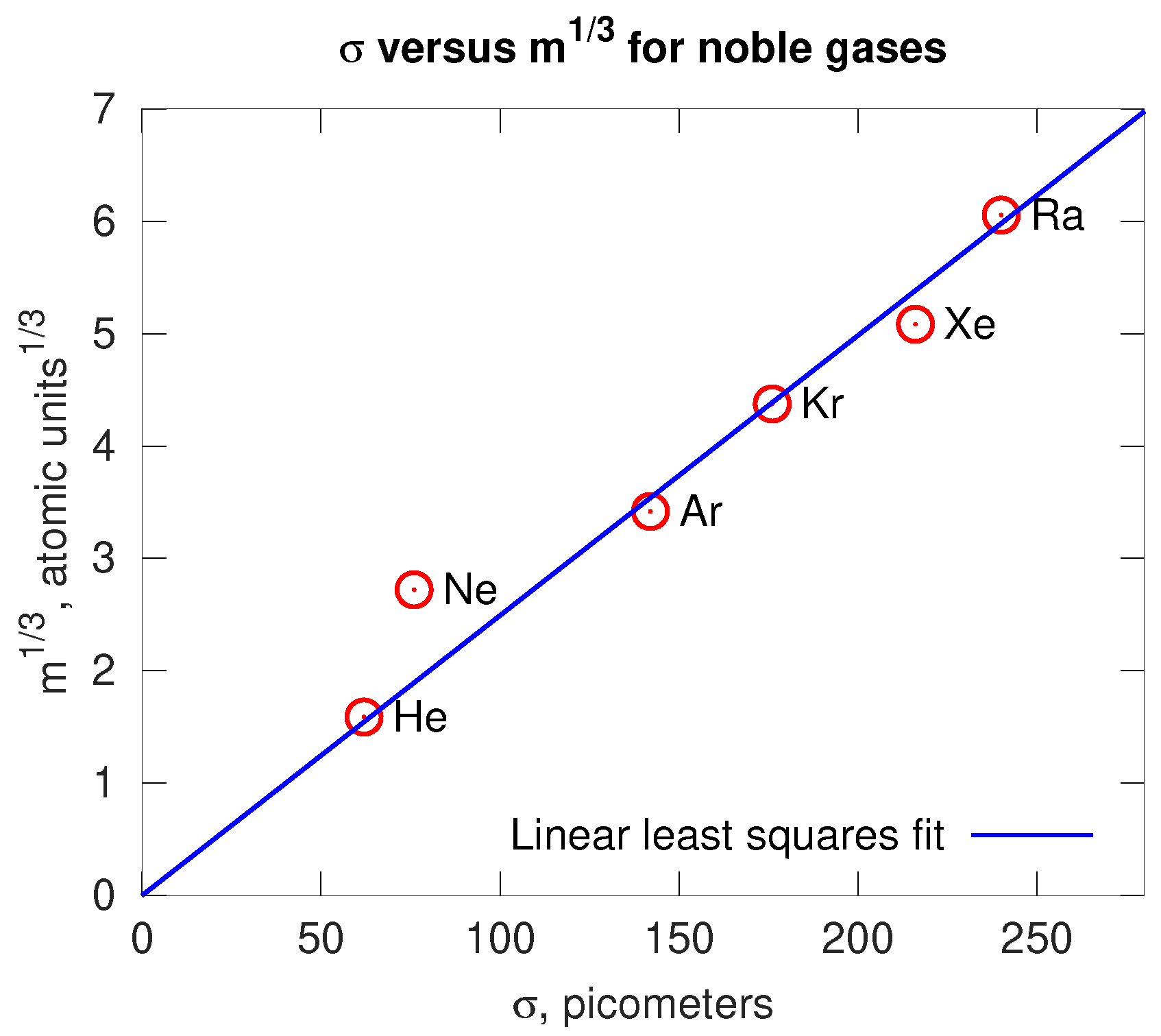
© 2019 by the author. Licensee MDPI, Basel, Switzerland. This article is an open access article distributed under the terms and conditions of the Creative Commons Attribution (CC BY) license (http://creativecommons.org/licenses/by/4.0/).
Share and Cite
MDPI and ACS Style
Abramov, R.V. The Random Gas of Hard Spheres. J 2019, 2, 162-205. https://doi.org/10.3390/j2020014
AMA Style
Abramov RV. The Random Gas of Hard Spheres. J. 2019; 2(2):162-205. https://doi.org/10.3390/j2020014
Chicago/Turabian StyleAbramov, Rafail V. 2019. "The Random Gas of Hard Spheres" J 2, no. 2: 162-205. https://doi.org/10.3390/j2020014
APA StyleAbramov, R. V. (2019). The Random Gas of Hard Spheres. J, 2(2), 162-205. https://doi.org/10.3390/j2020014