A Comparison of the Use of Pontryagin’s Maximum Principle and Reinforcement Learning Techniques for the Optimal Charging of Lithium-Ion Batteries

Abstract

Battery systems are one of the most important components for the development of flexible energy storage for future applications. These comprise energy storage in both the mobility sector and stationary applications. To ensure the safe operation of multiple battery cells connected in series and parallel in a battery pack, it is essential to implement state of charge (SOC) equalization strategies. Generally, two fundamentally different approaches can be distinguished. On the one hand, these are passive approaches for SOC equalization that are based on including additional Ohmic resistors in a battery back over which equalization currents flow as long as the correspondingly connected cells have different voltages. Despite the simple implementation of such equalization circuits, they have a major drawback, namely wasting stored energy to perform the SOC equalization. This waste of energy goes along with Ohmic heat production, which leads to the necessity of additional cooling for batteries with large power densities. On the other hand, active SOC equalization approaches have been investigated, which allow for an independent charging of the individual cells. Especially, this latter approach has big potential to be more energy efficient. In addition, the potential for a reduction of Ohmic heat production may contribute to extending the lifetime of battery cells. To perform the individual charging of battery cells in an energetically optimal manner, this paper provides a comparison of closed-form optimization approaches on the basis of Pontryagin’s maximum principle and approaches for reinforcement learning. Especially, their accuracy and applicability for the implementation of optimal online cell charging strategies are investigated.

1. Introduction

Lithium-ion batteries have become one of the most important enablers for the implementation of fully electric and hybrid traction systems in all domains of transportation [1,2,3,4]. These include individual transport in terms of electric bicycles [5], motorcycles [6], or cars [7], but also battery storage for all-electric ships [8], as well as electric and hybrid tramways and locomotives [9]. Besides the sector of transportation, Lithium-ion batteries are widely employed as energy storage for systems in consumer electronics, as well as battery storage power stations [10], in which they are employed as medium-time-scale buffers. Among others, the latter serve as systems that cover peak-power demands and allow for storing an excess amount of renewable energy, but can also be employed as equipment covering ancillary services in the domains of operating reserves, as well as frequency control in electric power grids and, thus, serving as a means to reduce the risk of power outage. Depending on the exact area of application, the capacities of these storage systems range from a few watt-hours up to the gigawatt-hour range.

Regardless of those different storage capacities, a common problem that all of these systems have to cope with is the equalization of the SOC of individual battery cells that are electrically connected in series and in parallel [11]. This SOC equalization is the prerequisite for the prevention of low discharge of individual cells or over-charging, which both may lead to irreversible damage of the cells in terms of capacity loss, accelerated degradation, and in the worst possible case, hazardous situations such as thermal runaway, which may lead to fires, exposing the technical equipment and the environment to high risks, causing extreme property and financial damage, and especially threatening the lives of humans [12].

Preventing low discharge and over-charging are typical functionalities of battery management systems. They are based on passive or active approaches for SOC equalization [11,13,14,15,16,17,18,19]. In the passive case, bleeder resistors can be included in battery packs (which can be activated and deactivated by means of semi-conductor switches) to equalize the voltage of individual cells that are compared with each other. The use of such resistors has the advantage of simple SOC equalization circuits. However, currents through these bleeder resistors lead to Ohmic heat production, which needs to be countered by cooling systems. In addition, wasting stored energy is inevitable by this kind of passive approach. In contrast, active approaches aim directly at charging (respectively, discharging) individual cells by decentralized sources. This active approach allows for implementing energy-optimal charging strategies, which are investigated in this paper from the point of view of minimizing the overall Ohmic heat production in terms of an energy equivalent when charging an individual cell from a given initial to a desired final SOC.

To account for the SOC-dependent nonlinearities of the dynamics of battery cells, this task is solved in this paper by means of two substantially different formulations. The first option is the derivation of optimal, finite-duration charging profiles with the help of Pontryagin’s maximum principle as an indirect optimization approach [20,21,22,23]. As an alternative, a direct control optimization is presented in terms of a reinforcement learning formulation [24,25]. The first alternative is further extended toward a predictive control technique [26,27]. It is additionally compared with a linear-quadratic regulator design [20,28]. For that purpose, it is assumed that the nonlinear equivalent circuit model forming the basis for the solution of the maximum principle is approximated by a linear time-invariant state-space representation for which an infinite time-horizon control is designed.

This paper is structured as follows. Section 2 gives a summary of an equivalent circuit representation of Lithium-ion batteries that has been identified experimentally in previous work [29]. The methodological foundations of the alternative optimization approaches, namely Pontryagin’s maximum principle and the reinforcement learning approach, are presented in Section 3 with a focus on energetically optimal battery charging. Representative simulation results, on the basis of the aforementioned experimentally validated battery model, are presented in Section 4, before conclusions and an outlook on future work are given in Section 5.

2. Equivalent Circuit Modeling and Criteria for the Energetically Optimal Charging of Lithium-Ion Batteries

In this section, the modeling assumptions for the dynamics of Lithium-ion batteries are described with a focus on the quantification of Ohmic losses occurring during instationary operating conditions.

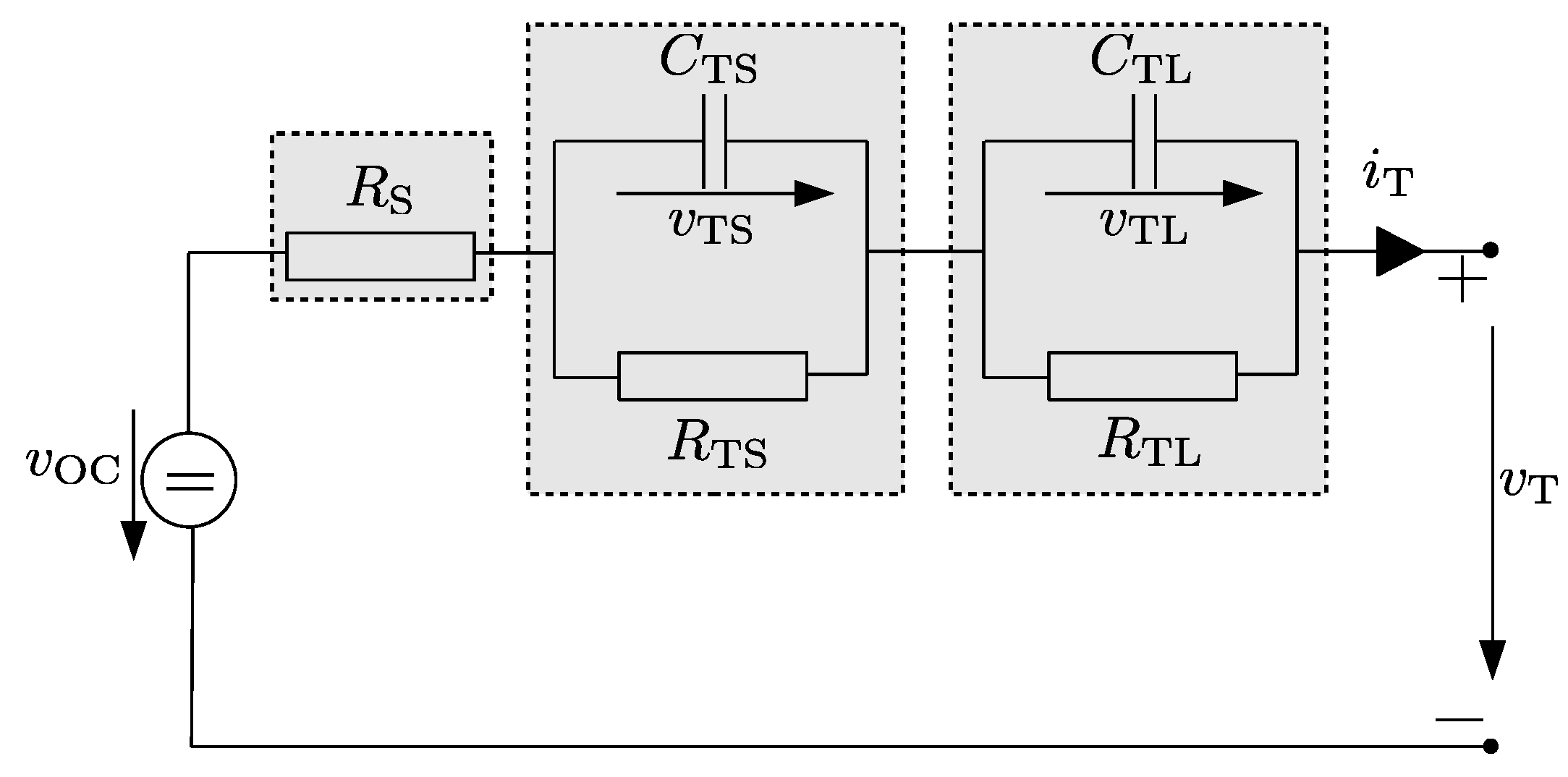
2.1. Equivalent Circuit Modeling

As described in a large variety of scientific articles (cf. [30,31]), equivalent circuit models with lumped, SOC-dependent resistances and capacitances are applicable to model the dynamics of charging and discharging Lithium-ion batteries. An illustration of the structure of the corresponding electric network is given in Figure 1.

Basically, these models can be transferred into a corresponding integer-order state-space representation, where the SOC $\sigma \left(t\right)$ and the voltages across a series connection of RC sub-networks serve as the state variables. In addition to the storage of charge carriers, represented by the SOC, the voltages across the RC sub-models are used to represent the dynamic phenomena that are caused by electro-chemical polarization effects and concentration losses with short and large time constants (denoted by the indices $\mathrm{TS}$ and $\mathrm{TL}$, respectively).

Under these considerations, the state vector of the equivalent circuit model is given by

$$\mathbf{x}\left(t\right)={\left[\begin{array}{ccc}\sigma \left(t\right)& v_{\mathrm{TS}}\left(t\right)& v_{\mathrm{TL}}\left(t\right)\end{array}\right]}^T$$

(1)

with the associated quasi-linear, continuous-time state equations

$$\begin{array}{cc}\hfill \dot{\mathbf{x}}\left(t\right)& =\mathbf{A}\left(\sigma \left(t\right)\right)·\mathbf{x}\left(t\right)+\mathbf{b}\left(\sigma \left(t\right)\right)·u\left(t\right)\hfill \\ \hfill & =\left[\begin{array}{ccc}0& 0& 0\\ 0& \frac{-1}{C_{\mathrm{TS}}\left(t\right)·R_{\mathrm{TS}}\left(t\right)}& 0\\ 0& 0& \frac{-1}{C_{\mathrm{TL}}\left(t\right)·R_{\mathrm{TL}}\left(t\right)}\end{array}\right]·\mathbf{x}\left(t\right)+\left[\begin{array}{c}\frac{-1}{C_{\mathrm{Bat}}}\\ \frac{1}{C_{\mathrm{TS}}\left(t\right)}\\ \frac{1}{C_{\mathrm{TL}}\left(t\right)}\end{array}\right]·u\left(t\right),\hfill \end{array}$$

in which the terminal current is the system input $u\left(t\right):=i_{\mathrm{T}}\left(t\right)$.

The first row of the state Equation (2) represents the integrating behavior

$$\dot{\sigma }\left(t\right)=-\frac{i_{\mathrm{T}}\left(t\right)}{C_{\mathrm{Bat}}}$$

(2)

between the charging/discharging current $i_{\mathrm{T}}\left(t\right)$ and the normalized SOC $\sigma \left(t\right)\in \left[0;1\right]$, where $C_{\mathrm{Bat}}$ is the nominal battery capacitance. Throughout this paper, $\sigma =1$ corresponds to the fully charged battery, while $\sigma =0$ is the operating condition of the completely discharged one.

The two further differential equations in the system model express the voltages $v_{\mathrm{TS}}\left(t\right)$ and $v_{\mathrm{TL}}\left(t\right)$ with the time constants [30,31]

$${\tau }_{\iota }=C_{\iota }\left(t\right)·R_{\iota }\left(t\right),\iota \in \{\mathrm{TS},\mathrm{TL}\},$$

(3)

which are temporally varying due to the SOC dependencies of the parameters

$$R_{\iota }\left(t\right)=R_{\iota \mathrm{a}}·e^{R_{\iota \mathrm{b}}·\sigma \left(t\right)}+R_{\iota \mathrm{c}}$$

(4)

and

$$C_{\iota }\left(t\right)=C_{\iota \mathrm{a}}·e^{C_{\iota \mathrm{b}}·\sigma \left(t\right)}+C_{\iota \mathrm{c}}.$$

(5)

Further SOC dependencies are relevant for the Ohmic series resistance

$$R_{\mathrm{S}}\left(t\right)=R_{\mathrm{Sa}}·e^{R_{\mathrm{Sb}}·\sigma \left(t\right)}+R_{\mathrm{Sc}},$$

(6)

as well as for the approximation

$$v_{\mathrm{OC}}\left(\sigma \left(t\right)\right)=v_0·e^{v_1·\sigma \left(t\right)}+\sum _{i=0}^3{v}_{i+2}·{\sigma }^i\left(t\right)$$

(7)

of the battery’s open-circuit voltage.

The latter, as well as the voltage drops $v_{\iota }\left(t\right)$, $\iota \in \{\mathrm{TS},\mathrm{TL}\}$, and the voltage drop over the series resistance $R_{\mathrm{S}}\left(t\right)$ can be combined with the help of Kirchhoff’s voltage law

$$v_{\mathrm{T}}\left(t\right)=v_{\mathrm{OC}}\left(t\right)-v_{\mathrm{TS}}\left(t\right)-v_{\mathrm{TL}}\left(t\right)-i_{\mathrm{T}}\left(t\right)·R_{\mathrm{S}}\left(t\right)$$

(8)

to find a relation between the terminal voltage $v_{\mathrm{T}}\left(t\right)$ and the terminal current $i_{\mathrm{T}}\left(t\right)$.

All parameters of the system model above can be identified experimentally, either by means of impedance spectroscopy or by using dedicated identification experiments such as those summarized in [29]. The parameter values listed in [29] are used in this paper for the numerical evaluation of the presented optimization approaches.

Remark 1. 

If the integer-order models mentioned before are not sufficiently accurate for describing long-term memory effects, they can be replaced with fractional-order differential equation models as presented, for example, in [32,33,34].

2.2. Quantification of Ohmic Losses

Ohmic losses in the battery, leading effectively to a change of its temperature, are caused by the electric currents through all Ohmic resistances in the equivalent circuit in Figure 1. Summing up the corresponding electric powers leads to the expression

$$P_{\mathrm{el}}\left(t\right)=R_{\mathrm{S}}\left(t\right)·i_{\mathrm{T}}^2\left(t\right)+\frac{v_{\mathrm{TS}}^2\left(t\right)}{R_{\mathrm{TS}}\left(t\right)}+\frac{v_{\mathrm{TL}}^2\left(t\right)}{R_{\mathrm{TL}}\left(t\right)},$$

(9)

which should be kept as small as possible when charging the battery from an initial SOC to a desired final one in a given time span. Besides a minimization of this power (in an integral sense over the complete charging duration), it is desired to limit the maximum absolute values of the charging currents. This latter aspect is accounted for in the following section by adding a penalty term to the cost function, which consists of the square of the control signal.

3. Optimal Control Synthesis

The optimal control design can be classified into indirect approaches (based on Pontryagin’s maximum principle [23]), which compute the optimal system inputs in terms of an auxiliary boundary value problem for the set of canonical equations, as well as into direct ones, which directly determine the system inputs (e.g., by using reinforcement learning [25]). This section summarizes the methodological foundations of these alternatives and further provides the link between an optimal open-loop control, as well as closed-loop feedback control techniques.

3.1. Indirect Optimization Using Pontryagin’s Maximum Principle

For the case of using Pontryagin’s maximum principle, we distinguish two different options for specifying the terminal system states. These are fixed terminal conditions for all state vector components in Section 3.1.1 and partially free ones in Section 3.1.2.

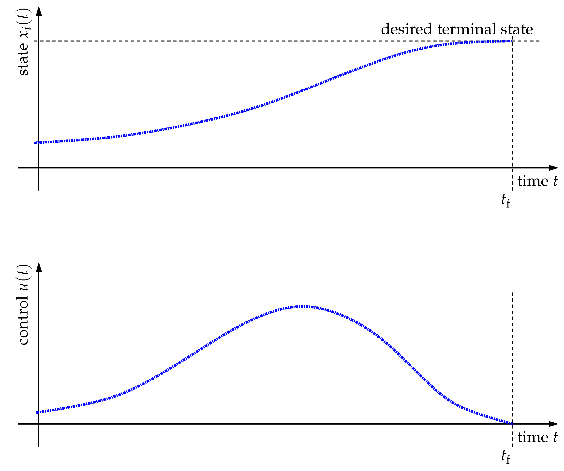
3.1.1. Fixed Terminal State

Assume a continuous-time system model

$$\dot{\mathbf{x}}\left(t\right)=\mathbf{f}(\mathbf{x}\left(t\right),u\left(t\right),t)$$

(10)

with the state vector $\mathbf{x}\left(t\right)\in {\mathbb{R}}^n$ and the scalar control signal $u\left(t\right)$. Assume further that the initial state is given by ${\mathbf{x}}_0=\mathbf{x}\left(t_0\right)$.

In the case of a predefined terminal state ${\mathbf{x}}_{\mathrm{f}}=\mathbf{x}\left(t_{\mathrm{f}}\right)$ at the time instant $t=t_{\mathrm{f}}>t_0$, the cost function to be minimized by the optimal control law

$$u^{*}\left(t\right)=u^{*}\left(\mathbf{x}\left(t\right),\mathbf{p}\left(t\right),t\right)$$

(11)

is given by

$$J\left(u\right)=\underset{t_0}{\overset{t_{\mathrm{f}}}{\int }}{f}_0(\mathbf{x}\left(\tau \right),u\left(\tau \right),\tau )\mathrm{d}\tau .$$

(12)

In (11), the vector $\mathbf{p}\left(t\right)\in {\mathbb{R}}^n$ denotes the co-state vector introduced in Pontryagin’s maximum principle according to [20,21,22,23].

In addition, the integrand

$$f_0(\mathbf{x}\left(t\right),u\left(t\right),t)=\alpha ·i_{\mathrm{T}}^2\left(t\right)+P_{\mathrm{el}}\left(t\right)$$

(13)

in Equation (12) corresponds to the electric power according to (9) with an additive penalty, where $\alpha >0$, that allows for limiting the control amplitudes. Note that time arguments are omitted in the following for the sake of compactness of the notation as long as the corresponding mathematical expressions are non-ambiguous. To find the candidate for the optimal control sequence $u^{*}$, the Hamiltonian

$$H\left(\mathbf{x},u,\mathbf{p},t\right)=-f_0(\mathbf{x},u,t)+{\mathbf{p}}^T·\mathbf{f}\left(\mathbf{x},u,t\right)$$

(14)

needs to be maximized according to

$$\underset{u\in \mathbb{R}}{max}\left(H\left(\mathbf{x},u,\mathbf{p},t\right)\right),$$

(15)

where we assume an unbounded control $u=u\left(t\right)\in \mathbb{R}$. Due to the unbounded control input and the differentiability of (16), the necessary optimality condition

$${\left.\frac{\partial H\left(\mathbf{x},u,\mathbf{p},t\right)}{\partial u}\right|}_{u=u^{*}}=-2\left(R_{\mathrm{S}}\left(t\right)+\alpha \right)i_{\mathrm{T}}\left(t\right)+{\mathbf{p}}^T\left(t\right)·\mathbf{b}\left(\sigma \left(t\right)\right)=0$$

(16)

leads to the unique solution candidate

$$u^{*}=\frac{1}{2\left(R_{\mathrm{S}}\left(t\right)+\alpha \right)}·{\mathbf{p}}^T\left(t\right)·\mathbf{b}\left(\sigma \left(t\right)\right),$$

(17)

representing the global maximum of the Hamiltonian due to the strict negativity of its second derivative

$$\begin{array}{c}\hfill {\left.\frac{{\partial }^{2}H\left(\mathbf{x},u,\mathbf{p},t\right)}{\partial u^2}\right|}_{u=u^{*}}=-2\left(R_{\mathrm{S}}\left(t\right)+\alpha \right)<0.\end{array}$$

(18)

To obtain a control law $u^{*}$ that minimizes Ohmic losses and penalizes the maximum control effort, the parameter

$$\alpha >0$$

(19)

is selected by a trial-and-error approach in this paper.

With the help of this optimized control, the set of canonical equations

$$\begin{array}{cc}\hfill \dot{\mathbf{x}}& =\frac{\partial H\left(\mathbf{x},u^{*},\mathbf{p},t\right)}{\partial \mathbf{p}}=\mathbf{f}\left(\mathbf{x},u^{*},t\right)\hfill \\ \hfill \dot{\mathbf{p}}& =-\frac{\partial H\left(\mathbf{x},u^{*},\mathbf{p},t\right)}{\partial \mathbf{x}}=\frac{\partial f_0}{\partial \mathbf{x}}-{\left(\frac{\partial \mathbf{f}(\mathbf{x},u^{*},t)}{\partial \mathbf{x}}\right)}^T·\mathbf{p}\hfill \end{array}$$

(20)

is obtained, which can be simplified according to

$$\begin{array}{cc}\hfill \dot{\mathbf{x}}& =\left[\begin{array}{ccc}0& 0& 0\\ 0& \frac{-1}{C_{\mathrm{TS}}\left(t\right)·R_{\mathrm{TS}}\left(t\right)}& 0\\ 0& 0& \frac{-1}{C_{\mathrm{TL}}\left(t\right)·R_{\mathrm{TL}}\left(t\right)}\end{array}\right]·\mathbf{x}+\left[\begin{array}{c}\frac{-1}{C_{\mathrm{Bat}}}\\ \frac{1}{C_{\mathrm{TS}}\left(t\right)}\\ \frac{1}{C_{\mathrm{TL}}\left(t\right)}\end{array}\right]·\frac{1}{2\left(R_{\mathrm{S}}\left(t\right)+\alpha \right)}·{\mathbf{p}}^T·\mathbf{b}\left(\sigma \left(t\right)\right)\hfill \\ \hfill \dot{\mathbf{p}}& =\left[\begin{array}{c}\frac{\partial P_{\mathrm{el}}\left(t\right)}{\partial \sigma }\\ \frac{2v_{\mathrm{TS}}\left(t\right)}{R_{\mathrm{TS}}\left(t\right)}\\ \frac{2v_{\mathrm{TL}}\left(t\right)}{R_{\mathrm{TL}}\left(t\right)}\end{array}\right]-{\left(\frac{\partial \mathbf{f}(\mathbf{x},u^{*},t)}{\partial \mathbf{x}}\right)}^T·\mathbf{p}.\hfill \end{array}$$

(21)

For this set of canonical equations, a boundary value problem needs to be solved with the $2n$ boundary conditions $\mathbf{x}\left(t_0\right)={\mathbf{x}}_0$ and $\mathbf{x}\left(t_{\mathrm{f}}\right)={\mathbf{x}}_{\mathrm{f}}$ in the case of fixed terminal states and perfectly known initial conditions. As shown in the following section, exactly prescribing all terminal state vector components ${\mathbf{x}}_{\mathrm{f}}$, especially the voltages across the RC sub-networks, leads to higher Ohmic losses than the case of partially free boundary conditions in the following section.

The typical choice of boundary conditions in this case is those of equilibria with different values for the SOC; hence,

$${\mathbf{x}}_0=\left[\begin{array}{c}{\sigma }_0\\ 0\\ 0\end{array}\right]\mathrm{and}{\mathbf{x}}_{\mathrm{f}}=\left[\begin{array}{c}{\sigma }_{\mathrm{f}}\\ 0\\ 0\end{array}\right].$$

(22)

3.1.2. Partially Free Terminal State

To avoid the exact prescription of an equilibrium state for the RC sub-network voltages, the second and third vector component of ${\mathbf{x}}_{\mathrm{f}}$ have to be left undefined. The correspondingly missing boundary conditions are then obtained after extending the cost function (12) by an additive term penalizing the final state according to

$$J_{\mathrm{h}}\left(u\right)=h_0(\mathbf{x}\left(t_{\mathrm{f}}\right),t_{\mathrm{f}})+\underset{t_0}{\overset{t_{\mathrm{f}}}{\int }}{f}_0(\mathbf{x}\left(\tau \right),u\left(\tau \right),\tau )\mathrm{d}\tau$$

(23)

with the typical choice

$$h_0(\mathbf{x}\left(t_{\mathrm{f}}\right),t_{\mathrm{f}})=\beta ·\left(v_{\mathrm{TS}}^2\left(t_{\mathrm{f}}\right)+v_{\mathrm{TL}}^2\left(t_{\mathrm{f}}\right)\right).$$

(24)

The terminal cost term in (24) leads to the transversality conditions [20,21,22,23]

$$\begin{array}{cc}\hfill p_2\left(t_{\mathrm{f}}\right)& =-{\left.\frac{\partial h_0(\mathbf{x},t_{\mathrm{f}})}{\partial v_{\mathrm{TS}}}\right|}_{\mathbf{x}=\mathbf{x}\left(t_{\mathrm{f}}\right)}=-2\beta v_{\mathrm{TS}}\left(t_{\mathrm{f}}\right)\hfill \\ \hfill p_3\left(t_{\mathrm{f}}\right)& =-{\left.\frac{\partial h_0(\mathbf{x},t_{\mathrm{f}})}{\partial v_{\mathrm{TL}}}\right|}_{\mathbf{x}=\mathbf{x}\left(t_{\mathrm{f}}\right)}=-2\beta v_{\mathrm{TL}}\left(t_{\mathrm{f}}\right)\hfill \end{array}$$

(25)

for two of the co-state variables to be considered in addition to the exactly defined terminal SOC

$$x_1\left(t_{\mathrm{f}}\right)={\sigma }_{\mathrm{f}}$$

(26)

when solving the boundary value problem for the canonical Equation (21).

3.2. Conversion into a Model Predictive Control Task

Both open-loop optimal control formulations from the previous subsection can be converted into appropriate model predictive control procedures. For that purpose, it is necessary to perform the optimization of the input sequence for the current state variables of the equivalent circuit, namely the SOC and the voltages across the RC sub-networks, after the previous optimization result has already been applied for a certain time interval. To perform the re-optimization, the equivalent circuit’s state variables are typically estimated by a suitable observer or filtering approach to provide the state estimates $\widehat{\mathbf{x}}\left(t_k\right)$ at the time instants $t_k$, $k\in \{0,1,\dots ,K_{\mathrm{c}}\}$. Widely applicable approaches, based on Kalman filters, neural networks, online estimation error minimization, or learning-type estimators can be found in [29,31,35,36,37,38,39,40]. Note that these estimation techniques are still an active field of research.

Figure 2 visualizes the computation of the optimal open-loop control sequence for the complete time horizon $\left[t_0;t_{\mathrm{f}}\right]$ with either of the formulations of Pontryagin’s maximum principle from the previous subsection. Due to the fact that this control sequence is then applied to the dynamic system without any further correction at runtime, it is not guaranteed that the desired terminal state (obtained perfectly by the prediction model employed for the offline optimization in the previous subsection) actually corresponds to the true terminal state. The reasons for this behavior are mismatches in the initial conditions, as well as imperfectly known system parameters and structural deviations between the assumed system dynamics and the true battery behavior.

Therefore, a predictive control setting can be implemented by following the strategies summarized in Figure 3. There, the open-loop control strategy is re-computed at each point of time $t_k$ in an online manner by using the same optimization approach as in the previous subsection. The corresponding input signal $u_k\left(t\right)$ is then applied to the system over the time interval $\left[t_k;t_{k+1}\right]$ before it is re-computed again with the new state estimates ${\widehat{x}}_i\left(t_{k+1}\right)$. Note that, in the implementation summarized in this figure, the prediction horizon becomes shorter after each control update. For noisy state estimates, used for the re-initialization of the optimization, this may have the drawback of large control variations towards the final time instant $t_{\mathrm{f}}$. This can be countered by increasing the penalty actor $\alpha$ when increasing k, by avoiding an exact specification of the final SOC, but rather penalizing it in the terminal costs (24), by switching to a constant voltage charging for higher values of the SOC or by switching to the state-feedback implementation presented in the following subsection when the time t approaches the final time instant $t_{\mathrm{f}}$.

3.3. Relations to Feedback Control Based on a Linear-Quadratic Regulator Design

The previous finite-horizon optimization problems can be turned into a closed-loop control approach by a minimization of the cost function

$$\overline{J}=\frac{1}{2}\underset{0}{\overset{\infty }{\int }}\left({\left(\mathbf{x}\left(\tau \right)-{\mathbf{x}}_{\mathrm{f}}\right)}^T·\mathbf{Q}·\left(\mathbf{x}\left(\tau \right)-{\mathbf{x}}_{\mathrm{f}}\right)+R{u}^2\left(\tau \right)\right)\mathrm{d}\tau .$$

(27)

Here, the vector ${\mathbf{x}}_{\mathrm{f}}$ corresponds to the terminal state constraint introduced in Section 3.1.1. The optimal controller is then given by the expression

$$u\left(t\right)={\mathbf{k}}^T\left({\mathbf{x}}_{\mathrm{f}}-\mathbf{x}\left(t\right)\right),$$

(28)

if the gain vector

$${\mathbf{k}}^T=R^{-1}{\mathbf{b}}^T\mathbf{P}$$

(29)

is computed in terms of the positive definite, state-independent solution of the algebraic Riccati equation

$${\mathbf{A}}^T\mathbf{P}+\mathbf{P}\mathbf{A}+\mathbf{Q}-\mathbf{P}\mathbf{b}{R}^{-1}{\mathbf{b}}^T\mathbf{P}=\mathbf{0},$$

(30)

where the weighting matrix $\mathbf{Q}$ and the scalar weight R are defined according to

$$\mathbf{Q}=\left[\begin{array}{ccc}\gamma & 0& 0\\ 0& {\displaystyle \frac{1}{{\overline{R}}_{\mathrm{TS}}}}& 0\\ 0& 0& {\displaystyle \frac{1}{{\overline{R}}_{\mathrm{TL}}}}\end{array}\right]$$

(31)

with the parameter

$$\gamma >0$$

(32)

as well as

$$R=\alpha +{\overline{R}}_{\mathrm{S}}.$$

(33)

Here, the parameter $\gamma$ is introduced in addition to the parameterization of the fundamental cost function in (12) to ensure that the state trajectory approaches the desired terminal state ${\mathbf{x}}_{\mathrm{f}}$.

Remark 2. 

State-dependent solutions of the algebraic Riccati equation, as introduced in [41,42,43], are not further studied in this paper because they can be interpreted as a refinement of the coarse state-independent solution of this subsection, which approaches the solution of Section 3.1.1 when setting the terminal time instant $t_{\mathrm{f}}$ to a large value.

Remark 3. 

A further combination of this state feedback controller with the optimization results of Pontryagin’s maximum principle is the use of the result $u^{*}$ of the open-loop optimization as a feedforward control signal, and to add a further feedback path that compensates the deviations between the offline optimized state trajectories and the currently estimated ones, see also Section 4.3.

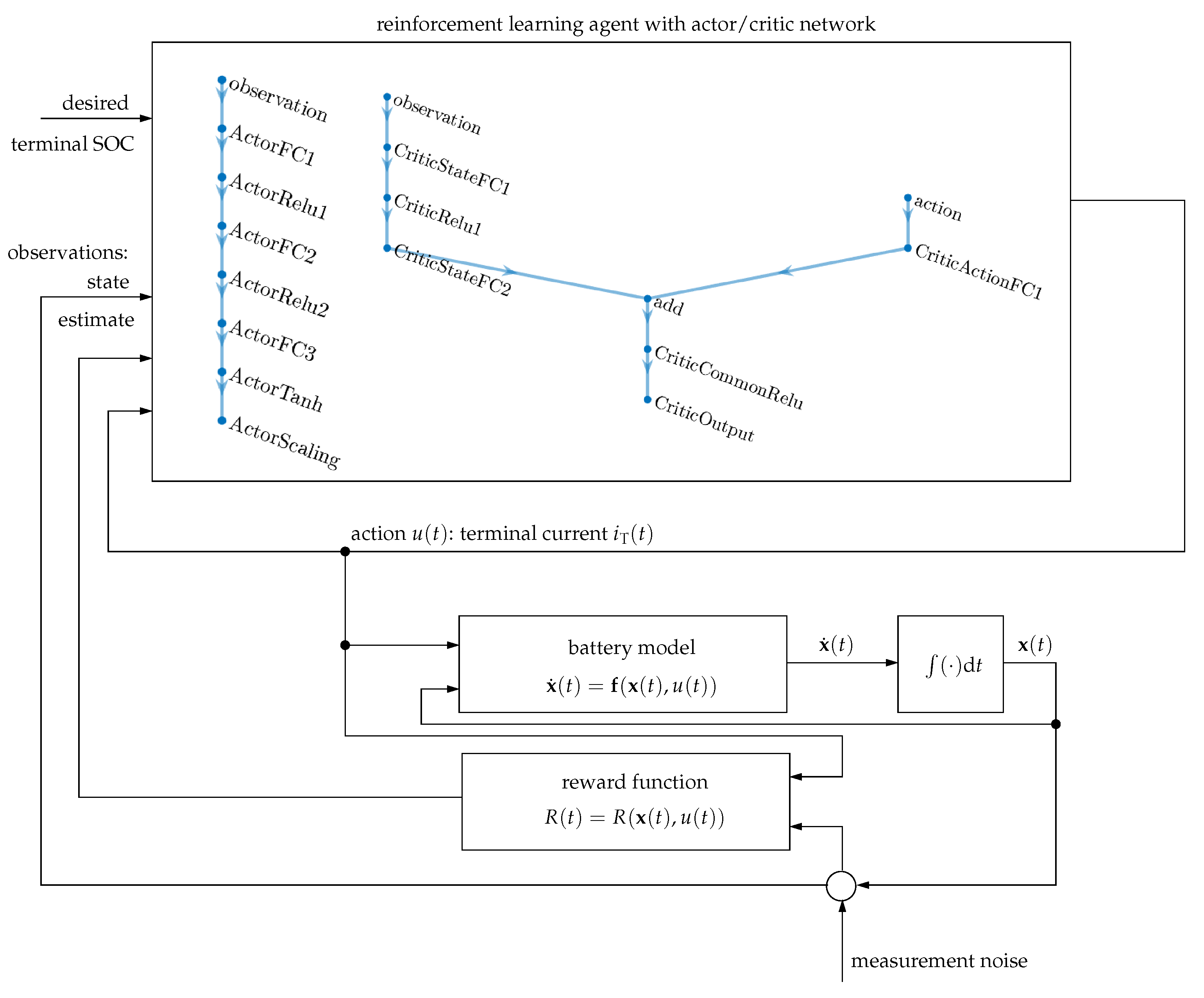
3.4. Direct Optimization by Reinforcement Learning

Reinforcement learning control approaches [24,25] can be used as an alternative to the solution techniques of the previous subsections to directly determine optimal control strategies. The general reinforcement learning environment, adapted to the case of optimal charging for Lithium-ion batteries, is summarized in Figure 4.

There, the reward function serves as a substitute for the performance criterion $J\left(u\right)$, where the quite commonly used notation is a maximization of the reward, as opposed to the minimization discussed before. Therefore, the basic constituent of the reward function is the multiplication of the electric power $P_{\mathrm{el}}$ (respectively, the integrand $f_0$ according to (13)) with a negative sign. As discussed in Section 4, it is extended by a penalization of the deviations of the actual SOC from the desired terminal state.

Due to the fact that the reinforcement learning approach avoids the solution of boundary value problems for a specific set of (estimated) initial states, it can be robustified directly by adding suitably chosen measurement noise (representing also the effect of state reconstruction errors in an aleatory form) in both the computation of the reward function and in the observation vector. In the application at hand, this observation vector corresponds to the full state vector consisting of the SOC and the voltages across the RC sub-networks of the equivalent circuit model in Figure 1.

The reinforcement learning itself, implemented as a deep deterministic policy gradient (DDPG) agent in Matlab within this paper, includes two neural networks:

• The actor network determines the control signal (action) in terms of the observations, where the individual layers in the network according to Figure 4 are fully connected layers denoted by FC and layers with ReLu and tanh activation functions;
• The critic network contains both observations and actions as inputs to determine the reward of the current policy, where the two corresponding input paths are superposed additively, as shown again in Figure 4.

3.5. Summary of the Properties of the Control Approaches

The fundamental properties of all control approaches presented in this section are summarized in

Table 1. Summary of the algorithmic properties of the considered control approaches.

Approach	Offline Effort	Online Effort	Robustness against Noise	Generalizability with Respect to Initial SOC	Optimization Efficiency
Maximum principle	medium	low	independent (pure offline solution)	low (recomputation required)	good
Predictive control	—	medium–high	depending on cost function parameters	excellent	excellent
Linear-quadratic feedback control	low	low	depending on cost function parameters	medium–good	low
Reinforcement learning	high	low–medium	high for sufficiently rich training data	good–excellent	excellent

. There, the characterization of the capability to minimize the Ohmic losses during the optimal charging, denoted as optimization efficiency, is based on the results presented in Section 4.

4. Simulation and Optimization Results

In this section, numerical simulation results are presented to illustrate the performance of the optimization approaches summarized in Section 3. The presentation of these results focuses on both the capability to transfer the Lithium-ion battery from a given SOC ${\sigma }_0$ to a desired terminal value ${\sigma }_{\mathrm{f}}$ in a fixed time span and to analyze the robustness against senor (respectively, state reconstruction) noise when adapting the control signal at runtime.

For all the following simulations, we assumed that the battery model according to Figure 1 is parameterized with the values listed in [29]. Moreover, the following initial and terminal conditions hold:

$${\sigma }_0=0.5\mathrm{and}{\sigma }_{\mathrm{f}}=0.9.$$

(34)

4.1. Indirect Optimization Using Pontryagin’s Maximum Principle

The numerical evaluation in this subsection is based on precomputing a charging profile for the Lithium-ion battery that transfers the initial SOC (${\sigma }_0$) to the final one (${\sigma }_{\mathrm{f}}$) in $3600\mathrm{s}$. This phase is followed by a relaxation phase of again $3600\mathrm{s}$ with the terminal current $i_{\mathrm{T}}\equiv 0\mathrm{A}$, which guarantees that the desired final SOC is kept, but that the voltages across both RC sub-networks approach zero, with a corresponding quantification of the additional Ohmic losses.

The corresponding results are summarized for two different values of the parameter $\alpha$ included in the cost function (13) in

Table 2. Ohmic losses (energy) during charging and relaxation phases for fixed terminal states.

$\mathit{\alpha }$	Losses during Charging ($\mathit{t}\in \left[0;3600\right]\mathbf{s}$)	Total Losses ($\mathit{t}\in \left[0;7200\right]\mathbf{s}$)
1	$843.11\mathrm{Ws}$	$843.16\mathrm{Ws}$
$0.01$	$841.26\mathrm{Ws}$	$841.32\mathrm{Ws}$

and 

Table 3. Ohmic losses (energy) during charging and relaxation phases for partially fixed terminal states with $\beta =50$.

$\mathit{\alpha }$	Losses during Charging ($\mathit{t}\in \left[0;3600\right]\mathbf{s}$)	Total Losses ($\mathit{t}\in \left[0;7200\right]\mathbf{s}$)
1	$690.14\mathrm{Ws}$	$702.62\mathrm{Ws}$
$0.01$	$686.13\mathrm{Ws}$	$702.52\mathrm{Ws}$

. It can be seen clearly that the partially free terminal states (penalized by the terminal cost according to (24)) lead to much smaller Ohmic losses than the case of setting all voltages exactly to zero at the end of the charging phase. For that reason, only the case of partially free terminal conditions is investigated further in the following graphical illustrations in Figure 5 and Figure 6.

The left column of these two figures corresponds to the case with the larger penalization of the charging current (larger value of $\alpha$) as compared to the right column. It can be seen that this larger value of $\alpha$ leads to a solution that is close to a constant current charging policy, which is additionally included in Figure 5a,b. For this constant current profile, the Ohmic losses in the pure charging phase result in $690.97\mathrm{Ws}$, while the overall losses including also the relaxation phase are $703.05\mathrm{Ws}$. It can be seen that these values are larger than the optimized charging profile, which is characterized (except for the very beginning and end) by currents that are smaller than the temporally constant alternative. Moreover, the remaining sub-graphs of Figure 5 and Figure 6 indicate the relaxation processes in the RC sub-networks after terminating the charging at $t=3600\mathrm{s}$. These results indicate also that too small values for $\alpha$ may lead to large current peaks at the end of the charging process, which need to be prevented by suitably selecting this parameter.

4.2. Model Predictive Control

As already discussed in Section 3.2, a pure offline optimization of the charging profile suffers from the disadvantage that it cannot adapt to uncertainty in the initial conditions, as well as to deviations of the actual battery parameters from the ones assumed for solving the optimization problem. Therefore, this subsection shows the results of a model predictive implementation of the optimal control law, where the duration $t_{k+1}-t_k$ between two points at which the control strategy is recomputed was set to $120\mathrm{s}$. At these points, knowledge about the current state vector $\widehat{\mathbf{x}}\left(t_k\right)$ is assumed to be known, which deviates, however, in the simulation by an additive zero-mean Gaussian noise from the true state values $\mathbf{x}\left(t_k\right)$ with a standard deviation of $0.01$ for the SOC and $0.001$ for both voltages.

The simulation results in Figure 7, again computed for $\alpha =0.01$ with the extended cost function that includes the terminal state penalization (24), contain in yellow color the one-standard-deviation bounds for the terminal current and the SOC, respectively, in addition to the corresponding average values. To obtain these one-standard-deviation bounds, the complete simulation was repeated 100 times.

Obviously, as also shown in Figure 8, the noise leads to the fact that the Ohmic losses in both the pure charging phase, as well as in the longer time span including the charging and relaxation phases become themselves uncertain; cf. Figure 8a,b. Moreover, also the desired terminal SOC is not reached perfectly at the final time instant $t_{\mathrm{f}}=3600\mathrm{s}$ according to Figure 8c. This latter aspect is re-discussed in the investigation of the reinforcement learning control approach, where it is shown that a remaining correction of the SOC for $t>3600\mathrm{s}$ in a few minutes leads to only small additional Ohmic losses.

4.3. Feedback Control Based on a Linear-Quadratic Regulator Design

Besides the use of a model predictive control approach, the design of a linear-quadratic state feedback controller is a further option to adapt the charging current to the state estimates of the battery equivalent circuit model at each point in time $t_k$. Using the same noise model as in the previous subsection and also a control update at integer multiples of $120\mathrm{s}$, the feedback controller derived in Section 3.3 with the parameters $\alpha =1$, $\gamma =100$, as well as ${\overline{R}}_{\mathrm{TS}}=R_{\mathrm{TS}}\left(0.7\right)$ and ${\overline{R}}_{\mathrm{TL}}=R_{\mathrm{TL}}\left(0.7\right)$ leads to the charging dynamics summarized in Figure 9.

As in the previous subsection, this simulation was repeated 100 times to quantify one-standard-deviation tolerance bounds for the terminal current $i_{\mathrm{T}}$ and for the SOC $\sigma$. Those tolerance bounds are shown in Figure 9 as the yellow bounds along the complete trajectory, as well as in the form of histograms in Figure 10 for the Ohmic losses and the SOC at the points of time $t=3600\mathrm{s}$ and $t=7200\mathrm{s}$.

It can be seen clearly that the feedback controller (based on the integral quadratic cost function) leads to significantly larger Ohmic losses than the previous two approaches. However, the advantage of this approach, becoming visible in Figure 10d, is the reduction of the remaining uncertainty of the SOC. For that reason, a practical application of this approach would be given by determining an optimal reference trajectory according to the offline evaluation of Pontryagin’s maximum principle (Section 3.1.2) and using the feedback controller to compensate the remaining deviations from the optimal (open-loop) charging profile. This approach will have similar Ohmic losses as the predictive controller presented in the previous subsection, however with the advantage of less online computational effort. Its disadvantage, however, will be the fact that the reference trajectory is restricted to a single initial point with a fixed charging duration, unless these are not pre-computed in a look-up-table-like manner for various initial SOC values and various process durations. This disadvantage can be avoided easily by the reinforcement learning approach investigated in detail in the following subsection.

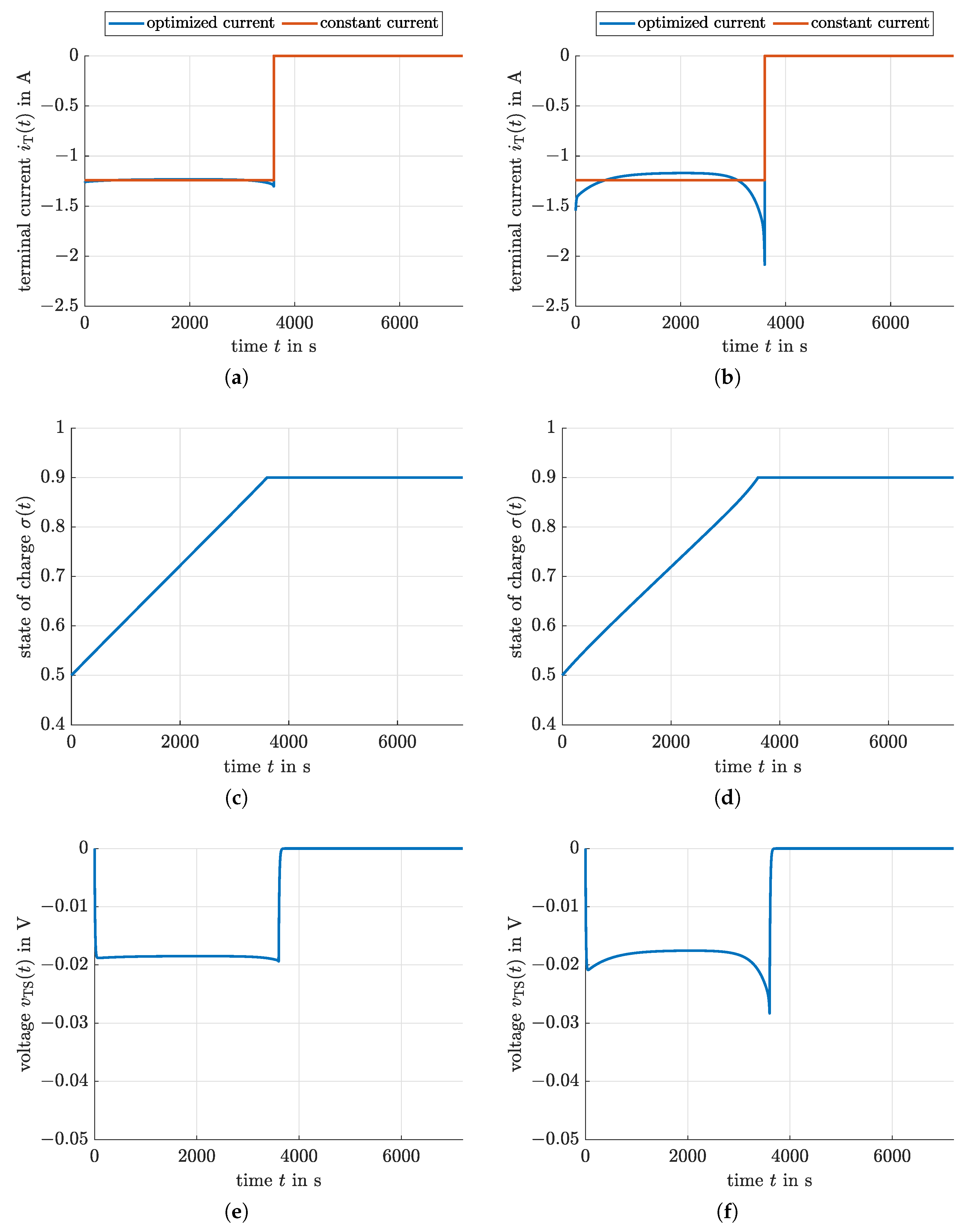
4.4. Optimized Charging Based on Reinforcement Learning

To implement a fundamental reinforcement learning control approach that is comparable with the previous subsections, assume a given initial SOC and the desired final SOC ${\sigma }_0$ and ${\sigma }_{\mathrm{f}}$, respectively. In addition, the charging duration is set to the fixed length of $3600\mathrm{s}$.

Now, a reinforcement learning environment is set up as shown in Figure 4 according to the details listed in Appendix A, where all relevant information concerning the numbers of neurons and the types of activation functions in each layer (both for the critic and actor networks), as well as the parameters of the learning agent are summarized in terms of Matlab code excerpts.

Note that the reinforcement learning control cannot guarantee a perfect SOC of ${\sigma }_{\mathrm{f}}$ at $t=3600\mathrm{s}$. Therefore, this time span is followed by a $120\mathrm{s}$ period with constant charging current to exactly achieve the desired SOC before the relaxation phase takes place until $t=7200\mathrm{s}.$

To make sure that the learning is close to the application of Pontryagin’s maximum principle discussed above, the running costs (included in the reward function) are chosen as in Equation (13) with $\alpha =1$, to which the additive time-dependent penalty term

$$5·{10}^3·{(\sigma \left(t\right)-{\sigma }_{\mathrm{f}})}^2·exp\left(\frac{t-3600}{50}\right)+{10}^4·\delta \left(t\right)$$

(35)

was added to obtain charging profiles approaching the desired SOC and, by means of

$$\delta \left(t\right)=\left\{\begin{array}{cc}{(\sigma \left(t\right)-0.05)}^2\hfill & \mathrm{for}\sigma \left(t\right)<0.05\hfill \\ {(\sigma \left(t\right)-0.95)}^2\hfill & \mathrm{for}\sigma \left(t\right)>0.95\hfill \\ 0\hfill & \mathrm{else},\hfill \end{array}\right.$$

(36)

preventing the optimizer from using control strategies violating the physical constraints on the SOC. Note that the scaling parameters in (35) were selected in such a way that undesired and physically meaningless solutions are penalized at least by one order of magnitude worse than the optimal control policies according to Section 3.1.2 and Section 3.2.

Using these settings, the results summarized in Figure 11 were obtained. In detail, Figure 11a,b indicate the case that the noise in Figure 4 is deactivated both during training and application of the trained agent.

Figure 11c,d contain the noise-free training and the evaluation of the learning agent with the same noise standard deviations that were also used in Section 4.2; finally, Figure 11e,f show the cases that the noise was active during the training and the application of the trained agents.

The corresponding Ohmic losses for these three different cases are summarized in

Table 4. Ohmic losses (energy) during the charging and relaxation phases for the different variants of the reinforcement learning control procedure.

Case According to	Losses during Charging ($\mathit{t}\in \left[0;3600\right]\mathbf{s}$)	Total Losses ($\mathit{t}\in \left[0;7200\right]\mathbf{s}$)
Figure 11a,b	$637.62\mathrm{Ws}$	$683.41\mathrm{Ws}$
Figure 11c,d	$636.43\mathrm{Ws}$	$685.61\mathrm{Ws}$
Figure 11e,f	$467.36\mathrm{Ws}$	$1163.7\mathrm{Ws}$

. It becomes obvious that these values are close to the solutions obtained by means of the offline control optimization (cf. Table 3) with the help of Pontryagin’s maximum principle and also the predictive control approach according to Figure 8. The big advantage of this solution is its small online computational effort (no boundary value problems have to be solved at runtime) and its simple generalizability to different charging durations and different initial conditions. To perform this generalization, it is only necessary to provide suitable observations to the reinforcement learning agent during the offline training. Future work concerning this task will especially deal with incorporating information on measurement uncertainty (as well as state reconstruction uncertainty) into the training, not only by the Gaussian noise processes used in Figure 11e,f, but also by set-valued counterparts. In addition, it will be investigated how the reward functions can be generalized reasonably to minimize the sensitivity of the resulting control approximation against such uncertainty, for example by directly including the noise-induced control signal variances as a further penalty term in the reward function.

Remark 4. 

It is possible that the total Ohmic losses over the complete time span $t\in \left[0;7200\right]\mathrm{s}$ for the reinforcement learning control approach are smaller than those for the offline-optimized solution using Pontryagin’s maximum principle. This is foremost caused by the fact that the terminal SOC is not predefined and that the additional $120\mathrm{s}$ time interval available for achieving the desired terminal SOC leads to a reduction of the maximum current, entering the expression for the Ohmic losses in a quadratic form.

5. Conclusions and Outlook on Future Work

In this paper, a thorough comparison between the use of Pontryagin’s maximum principle and reinforcement learning control approaches for the optimization of the charging strategies of Lithium-ion batteries was presented. This comparison was based on an experimentally validated equivalent circuit model. It was shown that the reinforcement learning control approach can achieve robust, close-to-optimal solutions despite the presence of state reconstruction noise if the utilized reward function for the learning agents is extended in a problem-specific manner.

Future work will especially aim at the consideration of more general uncertainty models included in the training phase, as well as the derivation of reinforcement-learning-based SOC equalization strategies when multiple Lithium-ion battery cells are electrically connected in series and in parallel.

References

1. Xiong, R.; He, H.; Guo, H.; Ding, Y. Modeling for Lithium-Ion Battery used in Electric Vehicles. Procedia Eng. 2011, 15, 2869–2874. [Google Scholar] [CrossRef] [Green Version]
2. Kennedy, B.; Patterson, D.; Camilleri, S. Use of Lithium-Ion Batteries in Electric Vehicles. J. Power Sources 2000, 90, 156–162. [Google Scholar] [CrossRef]
3. Han, U.; Kang, H.; Song, J.; Oh, J.; Lee, H. Development of Dynamic Battery Thermal Model Integrated with Driving Cycles for EV Applications. Energy Convers. Manag. 2021, 250, 114882. [Google Scholar] [CrossRef]
4. Pesaran, A.A. Battery Thermal Models for Hybrid Vehicle Simulations. J. Power Sources 2002, 110, 377–382. [Google Scholar] [CrossRef]
5. Liu, Y.C.; Chang, S.B. Design and Implementation of a Smart Lithium-Ion Battery Capacity Estimation System for E-Bike. World Electr. Veh. J. 2011, 4, 370–378. [Google Scholar] [CrossRef] [Green Version]
6. Nguyen, V.T.; Pyung, H.; Huynh, T. Computational Analysis on Hybrid Electric Motorcycle with Front Wheel Electric Motor Using Lithium Ion Battery. In Proceedings of the 2017 International Conference on System Science and Engineering (ICSSE), Ho Chi Minh City, Vietnam, 21–23 July 2017; pp. 355–359. [Google Scholar]
7. Chen, W.; Liang, J.; Yang, Z.; Li, G. A Review of Lithium-Ion Battery for Electric Vehicle Applications and Beyond. Energy Procedia 2019, 158, 4363–4368. [Google Scholar] [CrossRef]
8. Misyris, G.S.; Marinopoulos, A.; Doukas, D.I.; Tengnér, T.; Labridis, D.P. On Battery State Estimation Algorithms for Electric Ship Applications. Electr. Power Syst. Res. 2017, 151, 115–124. [Google Scholar] [CrossRef]
9. Haji Akhoundzadeh, M.; Panchal, S.; Samadani, E.; Raahemifar, K.; Fowler, M.; Fraser, R. Investigation and Simulation of Electric Train Utilizing Hydrogen Fuel Cell and Lithium-Ion Battery. Sustain. Energy Technol. Assess. 2021, 46, 101234. [Google Scholar] [CrossRef]
10. Feehall, T.; Forsyth, A.; Todd, R.; Foster, M.; Gladwin, D.; Stone, D.; Strickland, D. Battery Energy Storage Systems for the Electricity Grid: UK Research Facilities. In Proceedings of the 8th IET International Conference on Power Electronics, Machines and Drives (PEMD 2016), Glasgow, UK, 19–21 April 2016; pp. 1–6. [Google Scholar]
11. Cao, J.; Schofield, N.; Emadi, A. Battery Balancing Methods: A Comprehensive Review. In Proceedings of the IEEE Vehicle Power and Propulsion Conference, Harbin, China, 3–5 September 2008; pp. 1–6. [Google Scholar]
12. Zhang, X.; Li, L.; Zhang, W. Review of Research about Thermal Runaway and Management of Li-ion Battery Energy Storage Systems. In Proceedings of the 9th IEEE International Power Electronics and Motion Control Conference (IPEMC2020-ECCE Asia), Nanjing, China, 29 November–2 December 2020; pp. 3216–3220. [Google Scholar]
13. Wang, Q. State of Charge Equalization Control Strategy of Modular Multilevel Converter with Battery Energy Storage System. In Proceedings of the 5th International Conference on Power and Renewable Energy (ICPRE), Shanghai, China, 12–14 September 2020; pp. 316–320. [Google Scholar]
14. Speltino, C.; Stefanopoulou, A.; Fiengo, G. Cell Equalization in Battery Stacks Through State Of Charge Estimation Polling. In Proceedings of the 2010 American Control Conference, Baltimore, MD, USA, 30 June–2 July 2010; pp. 5050–5055. [Google Scholar]
15. Raeber, M.; Heinzelmann, A.; Abdeslam, D.O. Analysis of an Active Charge Balancing Method Based on a Single Nonisolated DC/DC Converter. IEEE Trans. Ind. Electron. 2021, 68, 2257–2265. [Google Scholar] [CrossRef] [Green Version]
16. Quraan, M.; Abu-Khaizaran, M.; Sa’ed, J.; Hashlamoun, W.; Tricoli, P. Design and Control of Battery Charger for Electric Vehicles Using Modular Multilevel Converters. IET Power Electron. 2021, 14, 140–157. [Google Scholar] [CrossRef]
17. Kim, T.; Qiao, W.; Qu, L. Series-Connected Self-Reconfigurable Multicell Battery. In Proceedings of the Twenty-Sixth Annual IEEE Applied Power Electronics Conference and Exposition (APEC), Fort Worth, TX, USA, 6–11 March 2011; pp. 1382–1387. [Google Scholar]
18. Ci, S.; Zhang, J.; Sharif, H.; Alahmad, M. A Novel Design of Adaptive Reconfigurable Multicell Battery for Power-Aware Embedded Networked Sensing Systems. In Proceedings of the IEEE GLOBECOM 2007—IEEE Global Telecommunications Conference, Washington, DC, USA, 26–30 November 2007; pp. 1043–1047. [Google Scholar]
19. Visairo, H.; Kumar, P. A Reconfigurable Battery Pack for Improving Power Conversion Efficiency in Portable Devices. In Proceedings of the 7th International Caribbean Conference on Devices, Circuits and Systems, Cancun, Mexico, 28–30 April 2008; pp. 1–6. [Google Scholar]
20. Stengel, R. Optimal Control and Estimation; Dover Publications, Inc.: Mineola, NY, USA, 1994. [Google Scholar]
21. Leitmann, G. An Introduction to Optimal Control; McGraw-Hill: New York, NY, USA, 1966. [Google Scholar]
22. Athans, M.; Falb, P.L. Optimal Control: An Introduction to the Theory and Its Applications; McGraw-Hill: New York, NY, USA, 1966. [Google Scholar]
23. Pontrjagin, L.S.; Boltjanskij, V.G.; Gamkrelidze, R.V.; Misčenko, E.F. The Mathematical Theory of Optimal Processes; Interscience Publishers: New York, NY, USA, 1962. [Google Scholar]
24. Buşoniu, L.; de Bruin, T.; Tolić, D.; Kober, J.; Palunko, I. Reinforcement Learning for Control: Performance, Stability, and Deep Approximators. Annu. Rev. Control 2018, 46, 8–28. [Google Scholar] [CrossRef]
25. Gosavi, A. Reinforcement Learning: A Tutorial Survey and Recent Advances. Informs J. Comput. 2009, 21, 178–192. [Google Scholar] [CrossRef] [Green Version]
26. Borrelli, F.; Bemporad, A.; Morari, M. Predictive Control for Linear and Hybrid Systems; Cambridge University Press: Cambridge, UK, 2017. [Google Scholar]
27. Maciejowski, J. Predictive Control with Constraints; Prentice Hall: Essex, UK, 2002. [Google Scholar]
28. Sontag, E. Mathematical Control Theory—Deterministic Finite Dimensional Systems; Springer: New York, NY, USA, 1998. [Google Scholar]
29. Reuter, J.; Mank, E.; Aschemann, H.; Rauh, A. Battery State Observation and Condition Monitoring Using Online Minimization. In Proceedings of the 21st International Conference on Methods and Models in Automation and Robotics, Miedzyzdroje, Poland, 29 August–1 September 2016. [Google Scholar]
30. Erdinc, O.; Vural, B.; Uzunoglu, M. A Dynamic Lithium-Ion Battery Model Considering the Effects of Temperature and Capacity Fading. In Proceedings of the International Conference on Clean Electrical Power, Capri, Italy, 9–11 June 2009; pp. 383–386. [Google Scholar]
31. Rauh, A.; Butt, S.; Aschemann, H. Nonlinear State Observers and Extended Kalman Filters for Battery Systems. Intl. J. Appl. Math. Comput. Sci. AMCS 2013, 23, 539–556. [Google Scholar] [CrossRef] [Green Version]
32. Hildebrandt, E.; Kersten, J.; Rauh, A.; Aschemann, H. Robust Interval Observer Design for Fractional-Order Models with Applications to State Estimation of Batteries. In Proceedings of the 21st IFAC World Congress, Berlin, Germany, 11–17 July 2020. [Google Scholar]
33. Wang, B.; Liu, Z.; Li, S.; Moura, S.; Peng, H. State-of-Charge Estimation for Lithium-Ion Batteries Based on a Nonlinear Fractional Model. IEEE Trans. Control Syst. Technol. 2017, 25, 3–11. [Google Scholar] [CrossRef]
34. Zou, C.; Zhang, L.; Hu, X.; Wang, Z.; Wik, T.; Pecht, M. A Review of Fractional-Order Techniques Applied to Lithium-Ion Batteries, Lead-Acid Batteries, and Supercapacitors. J. Power Sources 2018, 390, 286–296. [Google Scholar] [CrossRef] [Green Version]
35. Plett, G. Extended Kalman Filtering for Battery Management Systems of LiPB-Based HEV Battery Packs—Part 1. Background. J. Power Sources 2004, 134, 252–261. [Google Scholar] [CrossRef]
36. Plett, G. Extended Kalman Filtering for Battery Management Systems of LiPB-Based HEV Battery Packs—Part 2. Modeling and Identification. J. Power Sources 2004, 134, 262–276. [Google Scholar] [CrossRef]
37. Plett, G. Extended Kalman Filtering for Battery Management Systems of LiPB-Based HEV Battery Packs—Part 3. State and Parameter Estimation. J. Power Sources 2004, 134, 277–292. [Google Scholar] [CrossRef]
38. Bo, C.; Zhifeng, B.; Binggang, C. State of Charge Estimation Based on Evolutionary Neural Network. J. Energy Convers. Manag. 2008, 49, 2788–2794. [Google Scholar] [CrossRef]
39. Rauh, A.; Chevet, T.; Dinh, T.N.; Marzat, J.; Raïssi, T. Robust Iterative Learning Observers Based on a Combination of Stochastic Estimation Schemes and Ellipsoidal Calculus. In Proceedings of the 25th International Conference on Information Fusion (FUSION), Linkoping, Sweden, 4–7 July 2022; pp. 1–8. [Google Scholar]
40. Lahme, M.; Rauh, A. Combination of Stochastic State Estimation with Online Identification of the Open-Circuit Voltage of Lithium-Ion Batteries. In Proceedings of the 1st IFAC Workshop on Control of Complex Systems (COSY 2022), Bologna, Italy, 24–25 November 2022. [Google Scholar]
41. Friedland, B. Quasi-Optimum Control and the SDRE Method. In Proceedings of the 17th IFAC Symposium on Automatic Control in Aerospace, Toulouse, France, 25–29 June 2007; pp. 762–767. [Google Scholar]
42. Mracek, C.P.; Cloutier, J.R. Control Designs for the Nonlinear Benchmark Problem via the State-Dependent Riccati Equation Method. Int. J. Robust Nonlinear Control 1998, 8, 401–433. [Google Scholar] [CrossRef]
43. Çimen, T. State-Dependent Riccati Equation (SDRE) Control: A Survey. In Proceedings of the 17th IFAC World Congress, Seoul, South Korea, 6–11 July 2008; pp. 3761–3775. [Google Scholar]
Figure 1. Equivalent circuit model of a Lithium-ion battery in which a series connection of two RC sub-networks is used to represent lag phenomena in the charging and discharging phases.
Cleantechnol 04 00078 g001
Figure 2. Computation of the optimal feedforward control u ( t ) = u * ( r ) for the complete optimization horizon t 0 ; t f with the predicted optimal state trajectory x i ( t ) , i { 1 , , n } .
Cleantechnol 04 00078 g002
Figure 3. Re-computation of the optimal control sequences u k ( t ) for the reduced horizons t k ; t f , k { 0 , , K c } , with the associated predicted state trajectories x i , k ( t ) , i { 1 , , n } , initialized with the state estimates x ^ i ( t k ) .
Cleantechnol 04 00078 g003
Figure 4. Structure of the reinforcement learning environment.
Cleantechnol 04 00078 g004
Figure 5. Offline optimization of the charging profile according to Section 3.1.2. (a) Terminal current i T ( t ) for α = 1 ; (b) Terminal current i T ( t ) for α = 0.01 ; (c) SOC σ ( t ) for α = 1 ; (d) SOC σ ( t ) for α = 0.01 ; (e) Voltage v TS ( t ) for α = 1 ; (f) Voltage v TS ( t ) for α = 0.01 .
Cleantechnol 04 00078 g005
Figure 6. Offline optimization of the charging profile according to Section 3.1.2 (continued). (a) Voltage v TL ( t ) for α = 1 ; (b) Voltage v TL ( t ) for α = 0.01 ; (c) Terminal voltage v T ( t ) for α = 1 ; (d) Terminal voltage v T ( t ) for α = 0.01 .
Cleantechnol 04 00078 g006
Figure 7. Model predictive control under the influence of state reconstruction noise. (a) Terminal current i T ( t ) for α = 0.01 ; (b) SOC σ ( t ) for α = 0.01 .
Cleantechnol 04 00078 g007
Figure 8. Sensitivity of the Ohmic losses and the terminal SOC for the model predictive control. (a) Variability of the Ohmic losses occurring on the time interval t 0 ; 3600 s ; (b) Variability of the Ohmic losses occurring on the time interval t 0 ; 7200 s ; (c) Variability of the SOC at the end of the charging phase.
Cleantechnol 04 00078 g008
Figure 9. Feedback control under the influence of state reconstruction noise. (a) Terminal current i T ( t ) ; (b) SOC σ ( t ) .
Cleantechnol 04 00078 g009
Figure 10. Sensitivity of the Ohmic losses and the terminal SOC for the feedback control approach. (a) Variability of the Ohmic losses occurring on the time interval t 0 ; 3600 s ; (b) Variability of the Ohmic losses occurring on the time interval t 0 ; 7200 s ; (c) Variability of the SOC at t = 3600 s ; (d) Variability of the SOC at t = 7200 s .
Cleantechnol 04 00078 g010
Figure 11. Evaluation of the control optimization by means of reinforcement learning. (a) Terminal current i T ( t ) (optimization and evaluation without noise); (b) SOC σ ( t ) (optimization and evaluation without noise); (c) Terminal current i T ( t ) (optimization without noise; evaluation with noise); (d) SOC σ ( t ) (optimization without noise; evaluation with noise); (e) Terminal current i T ( t ) (optimization and evaluation with noise); (f) SOC σ ( t ) (optimization and evaluation with noise).
Cleantechnol 04 00078 g011