
Data-Driven Machine Learning Approach for Predicting the Higher Heating Value of Different Biomass Classes


 and
and
Abstract
:
1. Introduction
Relevant Literature and Study Novelty
- -
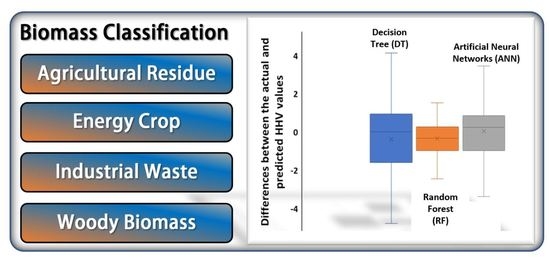
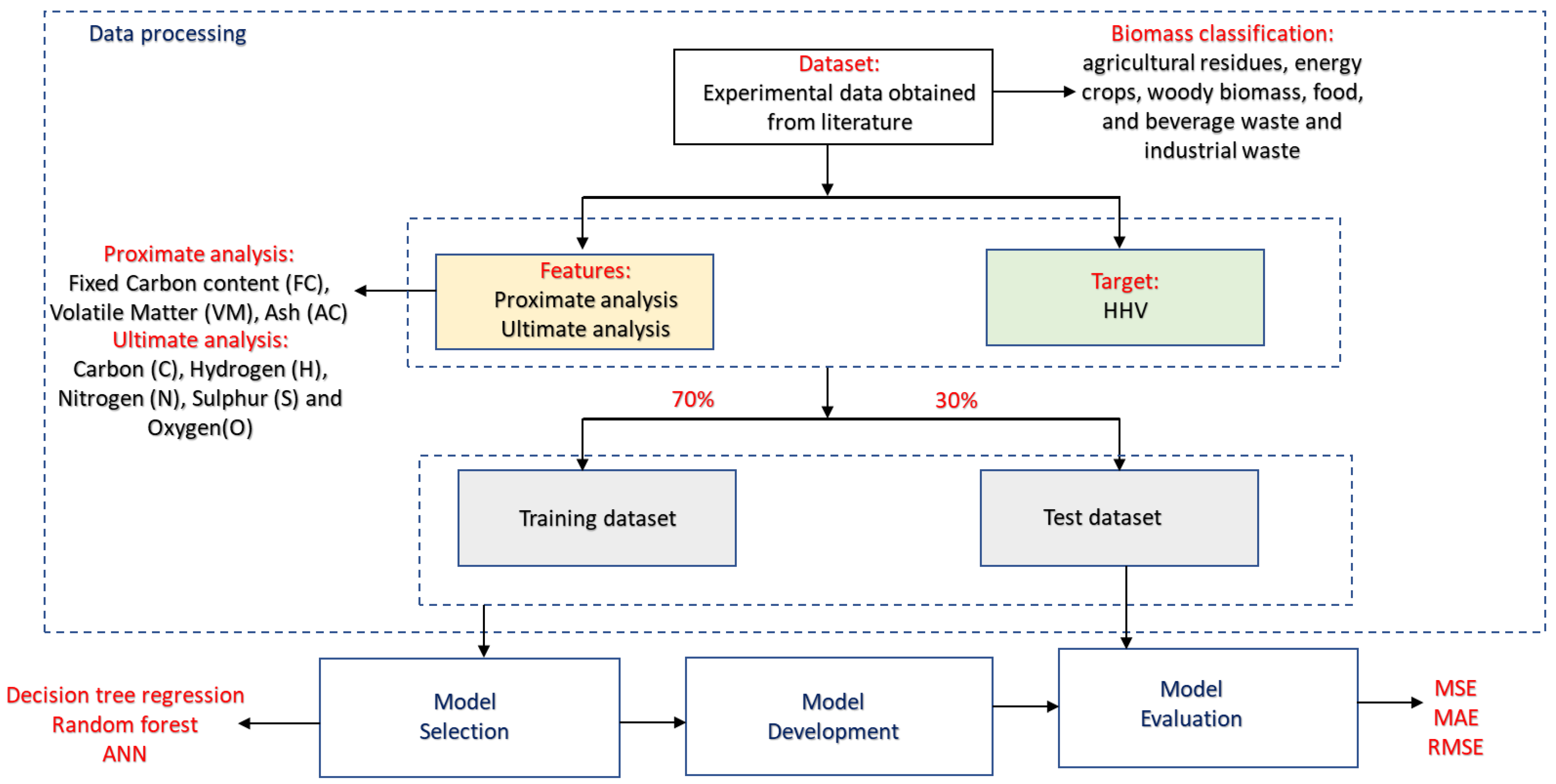
- This study proposes a comprehensive ML model comprising proximate and ultimate analysis and different biomass classification input features. Specifically, the biomass classification is selected to capture a wide range of materials, including agricultural residues, energy crops, woody biomass, and industrial waste.
- -
- This study applies a robust data set of 227 different biomass materials and computationally compares the performance of three different ML algorithms, including RF, DT, and ANN.
2. Methodology
2.1. Dataset Collection and Pre-Processing
2.2. Overview of the Machine Learning Algorithm
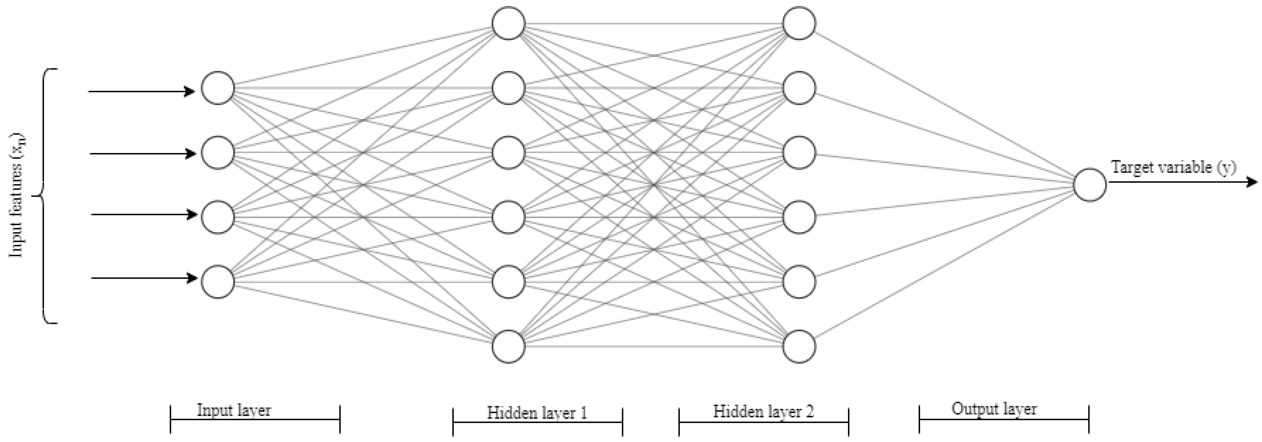
2.2.1. Artificial Neural Networks (ANN)
2.2.2. Decision Tree Regression (DT)
2.2.3. Random Forest (RF)
2.3. Empirical Correlations
3. Results and Discussion
3.1. Statistical Analysis of the Dataset
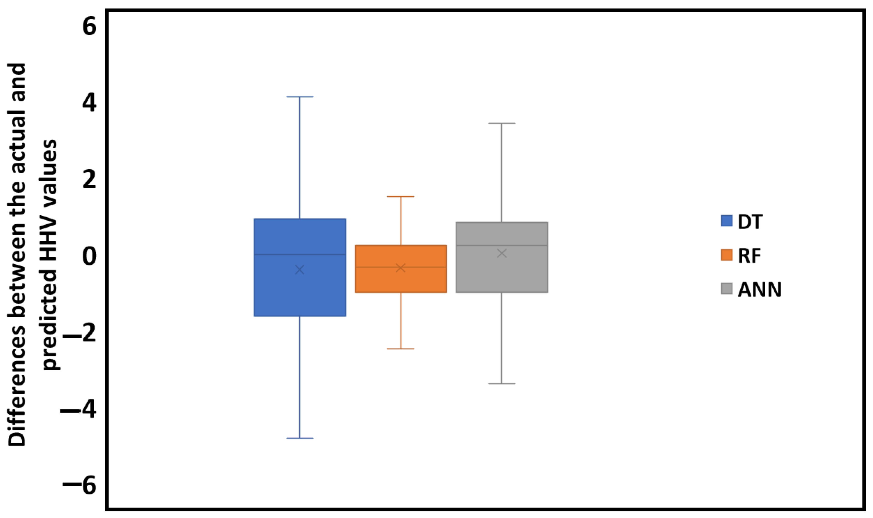
3.2. Model Performance Evaluation
3.3. Feature Analysis of the Best Model
3.4. Comparison of Other Models from Literature and Empirical Models
4. Conclusions
Supplementary Materials
Author Contributions
Funding
Institutional Review Board Statement
Informed Consent Statement
Data Availability Statement
Acknowledgments
Conflicts of Interest
Abbreviations
| AC | Ash content |
| ANN | Artificial neural network |
| ASTM | American Society for Testing and Materials |
| C | Carbon content |
| DT | Decision tree |
| FC | Fixed carbon content |
| H | Hydrogen content |
| HHV | Higher heating value |
| IEA | International Energy Agency |
| LHV | Lower heating value |
| MAE | Mean absolute error |
| ML | Machine learning |
| MSE | Mean Squared Error |
| N | Nitrogen content |
| O | Oxygen content |
| RF | Random Forest regression |
| RMSE | Root mean square error |
| S | Sulphur content |
| VM | Volatile matter |
References
- Okolie, J.A.; Nanda, S.; Dalai, A.K.; Kozinski, J.A. Hydrothermal gasification of soybean straw and flax straw for hydrogen-rich syngas production: Experimental and thermodynamic modeling. Energy Convers. Manag. 2020, 208, 112545. [Google Scholar] [CrossRef]
- IEA. International Energy Agency: Key World Energy Statistics. Statistics 2016, 78. Available online: http://www.oecd-ilibrary.org/energy/key-world-energy-statistics-2010_9789264095243-en (accessed on 3 June 2022).
- Cai, J.; He, Y.; Yu, X.; Banks, S.W.; Yang, Y.; Zhang, X.; Yu, Y.; Liu, R.; Bridgwater, A.V. Review of physicochemical properties and analytical characterization of lignocellulosic biomass. Renew. Sustain. Energy Rev. 2017, 76, 309–322. [Google Scholar] [CrossRef] [Green Version]
- Ohliger, A.; Förster, M.; Kneer, R. Torrefaction of beechwood: A parametric study including heat of reaction and grindability. Fuel 2013, 104, 607–613. [Google Scholar] [CrossRef]
- Channiwala, S.A.; Parikh, P.P. A unified correlation for estimating HHV of solid, liquid and gaseous fuels. Fuel 2002, 81, 1051–1063. [Google Scholar] [CrossRef]
- Friedl, A.; Padouvas, E.; Rotter, H.; Varmuza, K. Prediction of heating values of biomass fuel from elemental composition. Anal. Chim. Acta 2005, 544, 191–198. [Google Scholar] [CrossRef]
- Demirbaş, A. Calculation of higher heating values of biomass fuels. Fuel 1997, 76, 431–434. [Google Scholar] [CrossRef]
- Sheng, C.; Azevedo, J.L.T. Estimating the higher heating value of biomass fuels from basic analysis data. Biomass Bioenergy 2005, 28, 499–507. [Google Scholar] [CrossRef]
- Vaezi, M.; Passandideh-Fard, M.; Moghiman, M.; Charmchi, M. On a methodology for selecting biomass materials for gasification purposes. Fuel Process. Technol. 2012, 98, 74–81. [Google Scholar] [CrossRef] [Green Version]
- Yu, Z.T.; Xu, X.; Hu, Y.C.; Fan, L.W.; Cen, K.F. Prediction of higher heating values of biomass from proximate and ultimate analyses. Fuel 2011, 90, 1128–1132. [Google Scholar] [CrossRef] [Green Version]
- Qian, C.; Li, Q.; Zhang, Z.; Wang, X.; Hu, J.; Cao, W. Prediction of higher heating values of biochar from proximate and ultimate analysis. Fuel 2020, 265, 116925. [Google Scholar] [CrossRef]
- Choi, H.L.; Sudiarto, S.I.A.; Renggaman, A. Prediction of livestock manure and mixture higher heating value based on fundamental analysis. Fuel 2014, 116, 772–780. [Google Scholar] [CrossRef]
- Kieseler, S.; Neubauer, Y.; Zobel, N. Ultimate and proximate correlations for estimating the higher heating value of hydrothermal solids. Energy Fuels 2013, 27, 908–918. [Google Scholar] [CrossRef]
- Ighalo, J.O.; Adeniyi, A.G.; Marques, G. Application of linear regression algorithm and stochastic gradient descent in a machine-learning environment for predicting biomass higher heating value. Biofuels Bioprod. Biorefin. 2020, 14, 1286–1295. [Google Scholar] [CrossRef]
- Nieto, P.J.G.; García-Gonzalo, E.; Lasheras, F.S.; Paredes-Sánchez, J.P.; Fernández, P.R. Forecast of the higher heating value in biomass torrefaction by means of machine learning techniques. J. Comput. Appl. Math. 2019, 357, 284–301. [Google Scholar] [CrossRef]
- Taki, M.; Rohani, A. Machine learning models for prediction the Higher Heating Value (HHV) of Municipal Solid Waste (MSW) for waste-to-energy evaluation. Case Stud. Therm. Eng. 2022, 31, 101823. [Google Scholar] [CrossRef]
- Umenweke, G.C.; Afolabi, I.C.; Epelle, E.I.; Okolie, J.A. Machine learning methods for modeling conventional and hydrothermal gasification of waste biomass: A review. Bioresour. Technol. Rep. 2022, 17, 100976. [Google Scholar] [CrossRef]
- Xing, J.; Luo, K.; Wang, H.; Gao, Z.; Fan, J. A comprehensive study on estimating higher heating value of biomass from proximate and ultimate analysis with machine learning approaches. Energy 2019, 188, 116077. [Google Scholar] [CrossRef]
- Afolabi, I.C.; Popoola, S.I.; Bello, O.S. Modeling pseudo-second-order kinetics of orange peel-paracetamol adsorption process using artificial neural network. Chemom. Intell. Lab. Syst. 2020, 203, 104053. [Google Scholar] [CrossRef]
- Afolabi, I.C.; Popoola, S.I.; Bello, O.S. Machine learning approach for prediction of paracetamol adsorption efficiency on chemically modified orange peel. Spectrochim. Acta Part A Mol. Biomol. Spectrosc. 2020, 243, 118769. [Google Scholar] [CrossRef]
- Leng, E.; He, B.; Chen, J.; Liao, G.; Ma, Y.; Zhang, F.; Liu, S.; Jiaqiang, E. Prediction of three-phase product distribution and bio-oil heating value of biomass fast pyrolysis based on machine learning. Energy 2021, 236, 121401. [Google Scholar] [CrossRef]
- Li, J.; Zhu, X.; Li, Y.; Tong, Y.W.; Ok, Y.S.; Wang, X. Multi-task prediction and optimization of hydrochar properties from high-moisture municipal solid waste: Application of machine learning on waste-to-resource. J. Clean. Prod. 2020, 278, 123928. [Google Scholar] [CrossRef]
- Katongtung, T.; Onsree, T.; Tippayawong, N. Machine learning prediction of biocrude yields and higher heating values from hydrothermal liquefaction of wet biomass and wastes. Bioresour. Technol. 2021, 344, 126278. [Google Scholar] [CrossRef] [PubMed]
- Güleç, F.; Pekaslan, D.; Williams, O.; Lester, E. Predictability of higher heating value of biomass feedstocks via proximate and ultimate analyses—A comprehensive study of artificial neural network applications. Fuel 2022, 320, 123944. [Google Scholar] [CrossRef]
- Shenbagaraj, S.; Sharma, P.K.; Sharma, A.K.; Raghav, G.; Kota, K.B.; Ashokkumar, V. Gasification of food waste in supercritical water: An innovative synthesis gas composition prediction model based on Artificial Neural Networks. Int. J. Hydrogen Energy 2021, 46, 12739–12757. [Google Scholar] [CrossRef]
- Elmaz, F.; Yücel, Ö.; Mutlu, A.Y. Makine Öğrenmesi ile Kısa ve Elemental Analiz Kullanarak Katı Yakıtların Üst Isı Değerinin Tahmin Edilmesi. Int. J. Adv. Eng. Pure Sci. 2020, 32, 145–151. [Google Scholar] [CrossRef]
- Ozbas, E.E.; Aksu, D.; Ongen, A.; Aydin, M.A.; Ozcan, H.K. Hydrogen production via biomass gasification, and modeling by supervised machine learning algorithms. Int. J. Hydrogen Energy 2019, 44, 17260–17268. [Google Scholar] [CrossRef]
- Biau, G.; Devroye, L.; Lugosi, G. Consistency of random forests and other averaging classifiers. J. Mach. Learn. Res. 2008, 9, 2015–2033. [Google Scholar]
- Matin, S.S.; Chelgani, S.C. Estimation of coal gross calorific value based on various analyses by random forest method. Fuel 2016, 177, 274–278. [Google Scholar] [CrossRef]
- Parikh, J.; Channiwala, S.A.; Ghosal, G.K. A correlation for calculating HHV from proximate analysis of solid fuels. Fuel 2005, 84, 487–494. [Google Scholar] [CrossRef]
- Auret, L.; Aldrich, C. Interpretation of nonlinear relationships between process variables by use of random forests. Miner. Eng. 2012, 35, 27–42. [Google Scholar] [CrossRef]
- Ghugare, S.B.; Tiwary, S.; Elangovan, V.; Tambe, S.S. Prediction of Higher Heating Value of Solid Biomass Fuels Using Artificial Intelligence Formalisms. BioEnergy Res. 2013, 7, 681–692. [Google Scholar] [CrossRef]
- Tan, P.; Zhang, C.; Xia, J.; Fang, Q.Y.; Chen, G. Estimation of higher heating value of coal based on proximate analysis using support vector regression. Fuel Process. Technol. 2015, 138, 298–304. [Google Scholar] [CrossRef]
- Çakman, G.; Gheni, S.; Ceylan, S. Prediction of higher heating value of biochars using proximate analysis by artificial neural network. Biomass Convers. Biorefin. 2021, 1, 1–9. [Google Scholar] [CrossRef]
- Dai, Z.; Chen, Z.; Selmi, A.; Jermsittiparsert, K.; Denić, N.M.; Nešić, Z. Machine learning prediction of higher heating value of biomass. Biomass Convers. Biorefin. 2021, 1, 1–9. [Google Scholar] [CrossRef]


| Empirical Correlation | Equation for HHV in MJ/kg | Biomass Used | References |
|---|---|---|---|
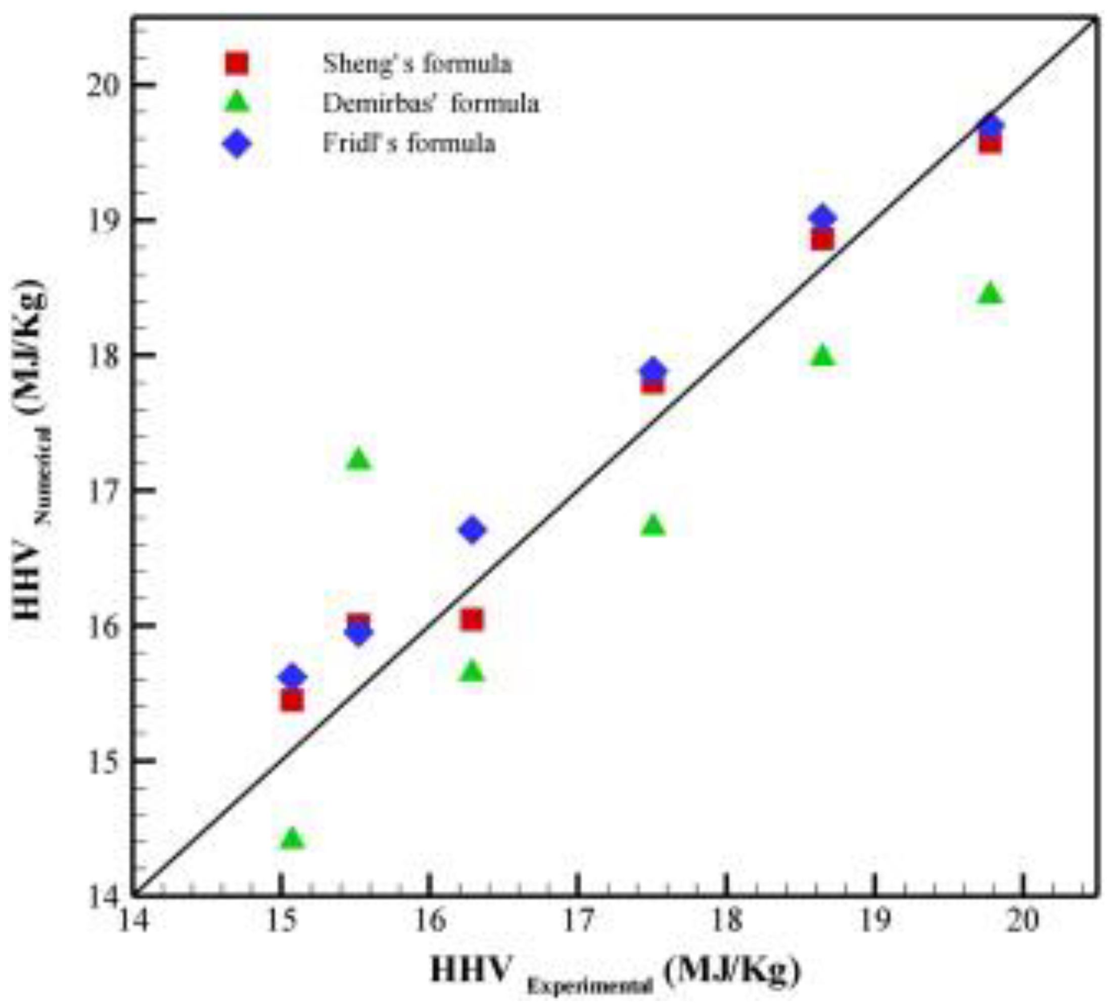
| Demirbas correlation | 0.01 (33.5C + 142.3H − 15.4O − 14.5 N) | Agricultural residues | Demirbaş [7] |
| Sheng correlation | −1.3675 + 0.3137C + 0.7009H + 0.0318O | Agricultural residues | Sheng and Azevedo [8] |
| Friedl correlation | 20600 + 3.55 C2 − 232C − 2230H + (51.2C × H) +131N | Wood, grass, rye, rape, reed, brewery waste, and poultry litter | Friedl et al. [6] |
| Yu correlation (Ultimate analysis) | 0.2949C + 0.8250H | Agricultural residues | Yu et al. [10] |
| Yu correlation (Proximate analysis) | 0.1905VM + 0.2521FC | Agricultural residues | Yu et al. [10] |
| Qian correlation (Ultimate analysis) | 32.9C + 162.7H − 16.2O − 954.4S + 1.408 | Biochars | Qian et al. [11] |
| Qian correlation (proximate analysis) | −30.3FC2 + 65.2Ash2 + 55.4FC − 48.5Ash + 9.591 | Biochars | Qian et al. [11] |
| ML Models | MAE | MSE | RMSE |
|---|---|---|---|
| DT | 1.48 | 4.36 | 2.09 |
| RF | 1.01 | 1.87 | 1.37 |
| ANN | 1.21 | 2.43 | 1.56 |
| Machine Learning Model | Input Feature | RMSE | References |
|---|---|---|---|
| RF | Proximate and ultimate analysis, biomass classes | 1.37 | This study |
| DT | Proximate and ultimate analysis, biomass classes | 2.09 | This study |
| ANN | Proximate and ultimate analysis, biomass classes | 1.56 | This study |
| ANN | Proximate analysis of biochars | 0.65 | Çakman et al., 2021 [34] |
| Extreme learning machine | Ultimate analysis | 1.93 | Dai et al. [35] |
| ANN | Ultimate analysis | 3.87 | Xing et al. [18] |
| RF | Ultimate analysis | 2.39 | Xing et al. [18] |
| SVM | Ultimate analysis | 2.53 | Xing et al. [18] |
| Genetic programming (GP) | Ultimate analysis | 0.95 | Ghugare et al. [32] |
| Multilayer perceptron neural network (MLP) | Ultimate analysis | 0.99 | Ghugare et al. [32] |
Publisher’s Note: MDPI stays neutral with regard to jurisdictional claims in published maps and institutional affiliations. |
© 2022 by the authors. Licensee MDPI, Basel, Switzerland. This article is an open access article distributed under the terms and conditions of the Creative Commons Attribution (CC BY) license (https://creativecommons.org/licenses/by/4.0/).
Share and Cite
Afolabi, I.C.; Epelle, E.I.; Gunes, B.; Güleç, F.; Okolie, J.A. Data-Driven Machine Learning Approach for Predicting the Higher Heating Value of Different Biomass Classes. Clean Technol. 2022, 4, 1227-1241. https://doi.org/10.3390/cleantechnol4040075
Afolabi IC, Epelle EI, Gunes B, Güleç F, Okolie JA. Data-Driven Machine Learning Approach for Predicting the Higher Heating Value of Different Biomass Classes. Clean Technologies. 2022; 4(4):1227-1241. https://doi.org/10.3390/cleantechnol4040075
Chicago/Turabian StyleAfolabi, Inioluwa Christianah, Emmanuel I. Epelle, Burcu Gunes, Fatih Güleç, and Jude A. Okolie. 2022. "Data-Driven Machine Learning Approach for Predicting the Higher Heating Value of Different Biomass Classes" Clean Technologies 4, no. 4: 1227-1241. https://doi.org/10.3390/cleantechnol4040075
APA StyleAfolabi, I. C., Epelle, E. I., Gunes, B., Güleç, F., & Okolie, J. A. (2022). Data-Driven Machine Learning Approach for Predicting the Higher Heating Value of Different Biomass Classes. Clean Technologies, 4(4), 1227-1241. https://doi.org/10.3390/cleantechnol4040075