Article

A Framework Based on Isoparameters for Clustering and Mapping Geophysical Data in Pedogeomorphological Studies

by
Gustavo Vieira Veloso
1,
Danilo César de Mello
1,
Heitor Paiva Palma
1,
Murilo Ferre Mello
1,
Lucas Vieira Silva
1,
Elpídio Inácio Fernandes-Filho
1,
Márcio Rocha Francelino
1,
Tiago Osório Ferreira
2,
José Cola Zanuncio
3,
Davi Feital Gjorup
1,
Roney Berti de Oliveira
4,
Marcos Rafael Nanni
4,
Renan Falcioni
4,* and
José A. M. Demattê
2
1
Department of Soil Science, Federal University of Viçosa, Campus Universitário, Av. Peter Henry Rolfs s/n, Viçosa 36570-900, MG, Brazil
2
Department of Soil Science, “Luiz de Queiroz” College of Agriculture (ESALQ), University of São Paulo, Av. Pádua Dias, 11, CP 9, Piracicaba 13418-900, SP, Brazil
3
Department of Entomology, Federal University of Viçosa, Campus Universitário, Av. Peter Henry Rolfs s/n, Viçosa 36570-900, MG, Brazil
4
Graduate Program in Agronomy, State University of Maringá, Av. Colombo, 5790, Maringá 87020-900, PR, Brazil
*
Author to whom correspondence should be addressed.
Soil Syst. 2025, 9(4), 124; https://doi.org/10.3390/soilsystems9040124 (registering DOI)
Submission received: 21 August 2025 / Revised: 17 October 2025 / Accepted: 4 November 2025 / Published: 8 November 2025
(This article belongs to the Special Issue Use of Modern Statistical Methods in Soil Science)

Abstract

Understanding soil variability supports improved land use and soil security. This study aimed to generate uniform geophysical classes by integrating data from three proximal geophysical sensors with synthetic soil and satellite images using machine learning, proposing a soil survey protocol. Geophysical data—natural gamma-ray emissions (eU, eTh, K40), magnetic susceptibility (κ), and apparent electrical conductivity (ECa)—were collected in Piracicaba, Brazil, and clustered into homogeneous geophysical-isoparameter classes. These classes were modeled alongside Synthetic Soil Images (SYSIs), Sentinel-2 (0.45–2.29 μm), Landsat (0.43–12.51 μm) imagery, and morphometric variables. Empirical validation compared the resulting geophysical-isoparameter map with conventional pedological and lithological maps. The Support Vector Machine (SVM) algorithm exhibited the best classification performance. Results demonstrated that geophysical sensors quantitatively and qualitatively capture soil attributes linked to formation processes and types. The geophysical-isoparameter map correlated well with pedological and lithological patterns. The proposed protocol offers soil scientists a practical tool to delineate soil and lithological units using combined sensor data. Promoting collaboration among pedologists, pedometric mappers, and remote sensing experts, this approach presents a novel framework to enhance soil survey accuracy and efficiency.

1. Introduction

In geography, isoparameters are used to represent zones of uniformity for a specific attribute, delineating areas that exhibit consistent values across a geographical landscape. A geophysical-isoparameter is defined as a spatially continuous unit characterized by statistically homogeneous combinations of geophysical variables (γ-ray spectrometry, magnetic susceptibility, and apparent electrical conductivity), together with satellite and morphometric covariates. These composite parameters capture the integrated geophysical signature of the landscape and act as proxy indicators of pedogenic and lithological processes. Through clustering and machine learning classification, geophysical-isoparameters can be used to delineate soil–lithological units with reduced subjectivity and improved quantitative reproducibility. This concept is particularly useful in soil surveying and mapping, as it facilitates the identification and analysis of regions with similar soil characteristics.
Soils are complex systems, having a great variability in physicochemical, mineralogical and biological attributes, both temporally and spatially [1], due to the varying interplays of soil-forming factors [2,3]. Hence, the understanding of soil spatial variability is essential to plan and achieve sustainable soil use and management [4]. Soil variability studies have been traditionally based on soil survey, mapping, and interpretation of data [5], but there are limitations related to financial and time constraints [6].
Remote sensing (RS) and proximal sensing (PS) have been used in soil survey and mapping, as well as spatial modeling due to the interaction between soil and many forms of energy detected [7]. Geophysical proximal sensors, such as gamma-ray spectrometry, magnetic susceptibility (κ), and apparent electrical conductivity (ECa), have recently found applications in soil science [8]. These sensors aid in comprehending soil processes and attributes by providing valuable data on soil properties and characteristics [9,10,11].
Gamma-ray spectrometry involves measuring natural gamma radiation emitted by potassium (K40), uranium (U238) and thorium (Th232), quantifying also the total radionuclides elements content, and total emissions from soil elements [12]. Soil magnetic susceptibility (κ) measures the magnetization capacity of soil particles due to ferrimagnetic minerals [13]. Soil apparent electrical conductivity (ECa) indicates the soil’s ability to conduct electricity [14]. The data obtained from the three sensors enable the assessment and inference of various pedological attributes, as well as pedogenic and surface processes associated with landscape dynamics [15,16].
Although remote sensing and proximal geophysical sensing datasets associated with machine learning have been widely used in geoscience, there are only few works that address the combined use of these techniques to discriminate soil attributes and types in pedological studies [8,17,18]. The combined use of these techniques can provide different datasets that relate to various soil characteristics and can facilitate cost-effective means to delineate management zones compared to traditional sampling methods, as well as prediction and spatialization of soil and lithology attributes that facilitate and refine current delineation methods in digital pedological and lithological mapping. However, the emerging generation of pedologists, blending pedometrics with traditional pedology, faces the challenge of establishing suitable protocols for pedological–lithological mapping.
Recent studies have increasingly explored the potential of integrating proximal geophysical sensors and machine learning techniques for digital soil mapping and pedological interpretation [8,17]. For example, gamma-ray spectrometry has been employed to evaluate weathering stages and mineralogical composition in tropical soils, demonstrating strong correlations with pedogenetic attributes such as clay content and base saturation [9,19,20,21]. Similarly, magnetic susceptibility has served as an effective proxy for inferring ferrimagnetic mineral content and identifying spatial trends related to pedogenetic and geomorphological processes [10,22,23]. Apparent electrical conductivity measurements have also been associated with soil texture, moisture, and salinity variations, offering valuable insights into subsurface heterogeneities [11,24,25]. When combined with satellite imagery and topographic variables, these sensor-derived datasets have shown promise in enhancing the resolution and accuracy of digital soil and lithology maps through machine learning approaches. However, despite these advancements, integrative frameworks that systematically combine multi-sensor geophysical data with remote sensing and machine learning to delineate homogeneous soil-lithological classes are still lacking. The present study aims to address this gap by proposing a novel protocol that synthesizes these techniques to improve classification accuracy and guide more efficient soil and geological surveys.
The debate persists among soil scientists about whether to concentrate on traditional coring or embrace more sophisticated proximate and remote sensing. Despite extensive efforts by the soil science community to enhance the utility of equipment in pedology, there is a lack of fundamental guidelines establishing standards for field operations that integrate different geophysical sensors, remote sensing, and machine learning techniques [16]. Consequently, formulating of effective strategies and protocols is crucial for the ongoing development of the pedological–lithological mapping community.
Integrating pedological and lithological attributes based on remote sensing and proximal sensing data provides substantial advantages over conventional geological surveys [15,16]. While traditional geological mapping typically focuses on rock structure and composition at broader spatial scales and emphasizes endogenous processes, the approach proposed herein enables the detection of more subtle surface variations critical for understanding pedological processes and land use planning. The combined use of geophysical sensors and satellite imagery facilitates a more detailed, dynamic, and cost-effective spatial characterization, allowing the identification of transition zones, surface heterogeneities, and pedological alterations that may not be detectable using geological variables or point-based attributes alone [8]. Thus, remote and proximal sensing technologies add significant value to the mapping process by enabling classification and high-resolution spatial modeling of homogeneous soil and lithological classes.
We aimed to propose a protocol for using proximal geophysical sensors and remote sensing techniques in soil survey work associated with machine learning, by focusing on the following topics: (i) to combine the use of geophysical data from proximal sensors to create homogeneous classes of geophysical parameters by machine learning; (ii) to use synthetic soil images and satellite images as covariates in modeling; (iii) to validate classes of geophysical parameters with pedological–lithological maps by analyzing the relationship between proximal and remote sensing.
Our primary hypothesis is that the integration of proximal geophysical sensors, satellite imagery, and morphometric variables can yield consistent “geophysical-isoparameters” that serve as valuable input data for soil type classification and serve as a base for a pedological–lithological survey and mapping.

2. Materials and Methods

2.1. Study Area

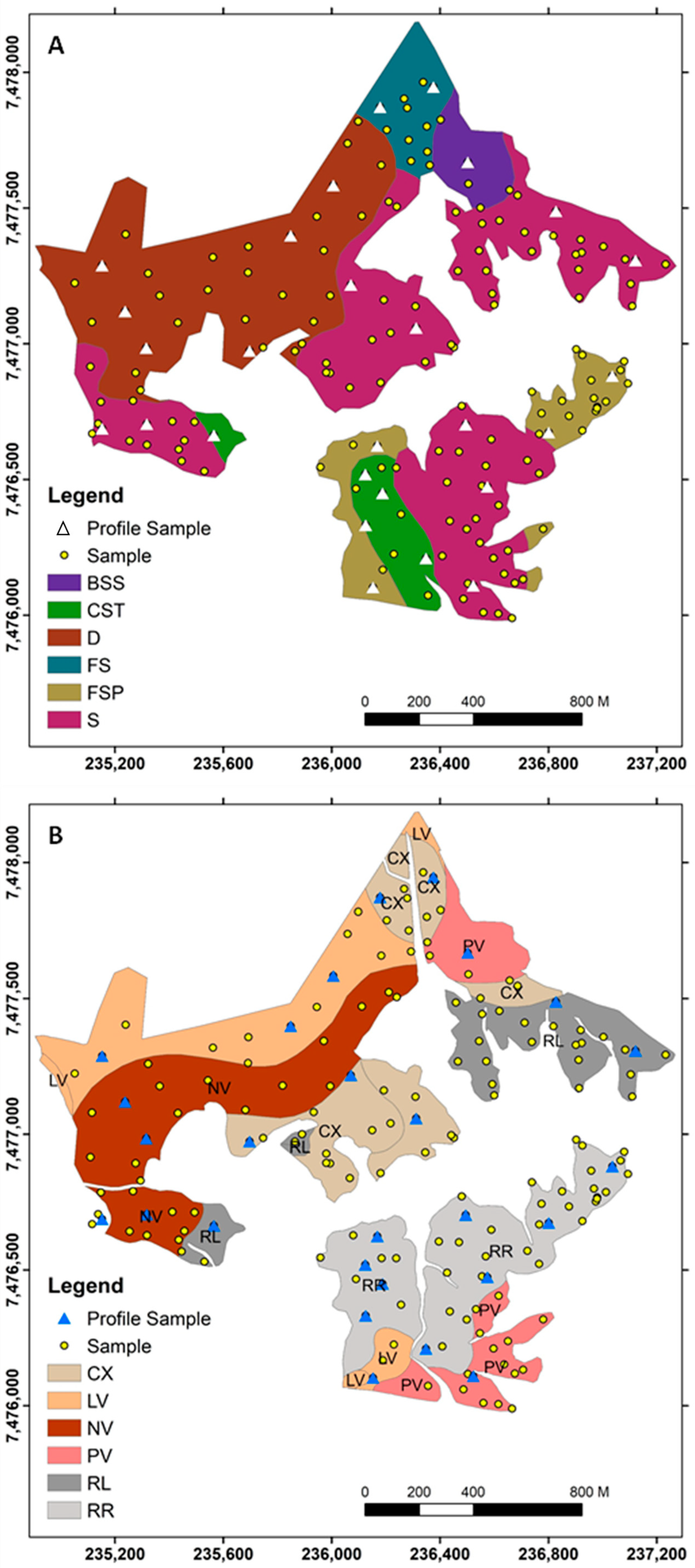
The research was undertaken in a rural area (165 ha) located at Piracicaba municipality, São Paulo state, Brazil (WGS 1984 −22.792333° S, −47.571245° W) (Figure 1). The elevation varies from 543 to 644 m, producing steep slopes, which contribute to soil variation. The area has a complex soils parent material, composed lithologically by igneous rock (basalts), sedimentary rocks (siltites and sandstones), basalt–siltite system (metamorphosed siltite) and, fluvial sediments (Figure 2B). The main soil types classified in study site, according to Bonfatti et al., (2020) [26] are: Rhodic Ferralsol, Rhodic Nitisol, Regosol Leptosol, Eutric Cambisol and, Rhodic Lixisol (Figure 2B). The pedological survey and mapping were conducted by a skilled pedologist utilizing a combination of remote sensing, fieldwork, and soil data at a scale of 1:10,000. The resulting maps were detailed, achieving a resolution of 30 m. The decision to select this area was primarily influenced by its landscape complexity, as we anticipated encountering a diverse range of parent materials and soil types, thereby enabling us to explore the potential of the sensor effectively. The lithological map was undertaken and detailed by Bonfatti (2020) [26]. with a scale of 1:100,000. However, we used an adapted map at 1:10,000 by an expert pedologist (Figure 2A).
The climate is subtropical mesothermal (Köppen classification) with average annual precipitation of 1200 mm and average temperatures of 18 °C in winter and 22° C in summer [27,28].

2.2. Acquisition of Proximal Geophysical Variables and Synthetic Soil Image (SYSI)

The geophysical measurement and soil samples were collected at 164 sample locations using three proximal geophysical sensors (Figure 1). The soil gamma-ray/radiometric, soil κ and soil ECa data were collected by using gamma-ray spectrometer (RS-230, Radiation Solutions Inc., Mississauga, ON, Canada), magnetic susceptibility meter (KT-10, Terraplus Inc., Richmond Hill, ON, Canada), conductivimeter (EM38, Geonics Limited, Mississauga, ON, Canada), respectively. The gamma-ray spectrometry corresponds to eU, eTh and K40 contents measurement. For more details on the collection, calibration methods and interpretation of results see Georesults (2021) [28].
The relationship and the ratios between the following radionuclides were calculated: eTh/K40; eU/K40; and (eU + eTh)/K40 (Table 1). In addition, four ratios between geophysical variables related to κ were calculated: K40/κ; eTh/κ; eU/κ and κ/ECa (Table 1). The calculations of these relationships aimed to acquire a more extensive range of information concerning the utilized sensors [29].
One of the main challenges in remote sensing for soil mapping, particularly in regions with dense and persistent vegetation cover, is the potential introduction of vegetation artifacts that can obscure or misrepresent underlying lithological features. This issue raises concerns about the reliability of satellite-derived data in accurately capturing soil properties. We implemented the Synthetic Soil Image (SYSI) approach to address this. SYSI is constructed by aggregating multispectral images from satellites such as Landsat and Sentinel, acquired over several years, and selectively compositing scenes with minimal vegetation cover, thereby capturing periods of bare soil exposure [30]. This technique is especially effective in tropical regions like Brazil, where consistent vegetation (agriculture or forests) can present significant obstacle to conventional soil analysis. By minimizing vegetation interference, SYSI enhances the visibility of soil spatial variability and supports more precise characterization of attributes such as texture, mineralogy, and fertility [31]. These synthetic images thus provide robust inputs for machine learning models applied in digital soil mapping, crop modeling, and environmental monitoring, ensuring more accurate predictions and reducing the risk of vegetation-induced biases.
To generate the SYSI, the GEOS3 methodology was used [31]. This method involved filtering the images from Landsat 5 satellite to extract only those captured during the dry season in the study area. Additionally, other objects in the area, apart from the soil, were filtered out. The GEOS3 method utilized satellite images representing dry seasons spanning from 1984 to 2011, selected due to reduced cloud coverage, a higher incidence of bare soil areas, and a diminished influence of moisture in the soil surface layer. The application of the GEOS3 technique during the dry season, when precipitation is virtually absent in the southeast and south of Brazil (except for rare extreme weather events related to global warming), minimizes the influence of soil moisture variability, thereby ensuring more uniform conditions for SYSI acquisition. For further details on the GEOS3 method, please refer to the additional information available in Demattê (2018) [31].
Here, the exclusion of vegetation indices (e.g., NDVI, SAVI, EVI) was intentional to maintain consistency with the SYSI approach, which minimizes vegetation and moisture interference by focusing on bare-soil reflectance. This design ensures that the modeled relationships reflect soil spectral and geophysical properties rather than vegetation dynamics. Nevertheless, in regions where complete bare-soil exposure is uncommon, vegetation indices could provide complementary, indirect information about soil properties. The proposed protocol can therefore be most effectively applied under conditions of partial or total soil exposure, while remaining adaptable for future integration of vegetation metrics where appropriate.

2.3. Satellite Images, Digital Elevation Model, and Morphometric Data

The spectral covariates (Table 2) were obtained by MSI (Multi Spectral Instrument) sensors coupled to the Sentinel-2 orbital system, and OLI (Operational Land Imager) and TIRS (Thermal Infrared) sensors coupled to the Landsat8 orbital system. Ten bands from the Sentinel-2 and 13 bands from Landsat 8 were used (Table 2). The satellite images were acquired between the months of June and July 2018 (mosaic). The satellite bands were resampled to 30 m pixels, using the raster package [32] in the R-software version 4.3.2 [33].
All images were cloud-filtered using built-in quality assurance (QA) bands. For Landsat 8, we applied the QA_PIXEL band to mask out clouds, cloud shadow, and snow. For Sentinel-2, we used the SCL (Scene Classification Layer) to remove cloud and water pixels. We did not apply additional filtering for vegetation or soil moisture, as our goal was to capture natural spectral variability across land cover types. We selected images from June to July 2018 to ensure minimal seasonal and atmospheric variation. In addition, this month represents the peak of the dry season, during which precipitation is virtually absent. This ensures relatively stable soil moisture conditions, which is important for SYSI measurements and geophysical sensor readings. The final mosaic was built using the best-available scenes from that period, prioritizing low cloud cover. Specific acquisition dates are now listed in the revised Table 2. All bands were resampled to a spatial resolution of 30 m to ensure compatibility across sensors. Sentinel-2 bands with higher resolution were downscaled; coarser thermal bands from Landsat were excluded from predictor selection to avoid spatial mismatch.
The digital elevation model (DEM) was generated utilizing a 1:10,000 scale planialtimetric map as the foundational base map, supplemented with 5 m contour lines. ESRI ArcGIS 10.4 software was employed for data geoprocessing purposes. This foundational map was originally compiled by the Campinas Geographic Institute (IGC). Subsequently, the finalized DEM was exported with a resolution set at 30 m. From the final DEM, 48 additional morphometric variables (Table 3) were extracted in R software (R Core Team, 2023) [32]. The spectral and morphometric covariates (Table 2 and Table 3, respectively), were grouped with the SYSI bands forming the base dataset for input into the modeling process.
All the sensor data values (from Table 1) were concatenated with the geographic coordinates of the 164 observation points. The geographic coordinates of the 164 points sampled were used to extract the values of the spectral and morphometric rasters. 21 variables derived from morphometric data and 29 variables from spectral data were also obtained, in addition to X and Y coordinates, totaling 52 variables. After that, the values of the morphometric and spectral covariates were extracted from all 164 collection points in R software [33]. This dataset (groups of predefined parameter values and covariate values) was used to create the final database for the modeling process.

2.4. Geophysical-Isoparameters, Principal Component Analysis and Modeling Process

We used the expression “geophysical-isoparameters” to refer to homogeneous classes of geophysical data, which are the results of the grouping of eU, eTh, K40, κ, and ECa. These homogeneous classes of geophysical parameters presented the smallest intragroup variation, maximum intergroup variation, and a high association with pedological and lithological classes.
The modeling process for generating the “geophysical-isoparameters” is illustrated in the flowchart (Figure 3) and can be categorized into four distinct phases: determining the number of clusters, covariate selection, training/testing, and spatialization. All processing was undertaken in R software [32,33,34].
The Principal Component Analysis (PCA) method was conducted using 12 parameters obtained from the geophysical dataset applied to all sampled points (164) (Table 1). PCA employs a linear transformation to orthogonal data, resulting in a new set of data called principal components (PCs). These PCs were used to explain the observed variation in the data, and are also used for data clustering [34]. Four principal components (PCs) were identified as the ideal set and subsequently used in the following steps. PCA was applied only to the geophysical dataset to generate clusters using the k-means method. At the same time, information from the Landsat and Sentinel satellites was directly incorporated into the model as covariates.
The ideal cluster number was selected by assessing homogeneity, specifically by identifying the minimum value assessing the Scattering-Density Index (“SDindex”) between the tested groups [35]. The Scattering-Density Index, introduced by Halkidi et al. (2000) [34], is a cluster validity measure that simultaneously evaluates intra-cluster compactness (density) and inter-cluster separation (scattering), providing a comprehensive assessment of clustering quality. This process was conducted in R software, using the NbClust function from the “NbClust” package [36]. Consequently, a total of five clusters were designated as the optimal number of classes. The data used in the cluster analysis were those generated by the PCA. In conjunction with the four principal components (PCs) generated in the preceding step, the optimal number of clusters was employed to form groups characterized by similar geophysical data values within each group, yet distinct between the groups. This processing phase involved employing the k-means grouping method, specifically utilizing the “k-means” function within the R software package [33].

2.5. Selection of Covariates

The covariate selection process was carried out by using Caret package [37] in R software (R Core Team, 2023) and this process involves three phases to streamline the final model and reduce computational effort and time. In the initial phase, covariates exhibiting no variability were eliminated based on their sampling variance, calculated using values extracted from the specific sampling point locations within the complete input dataset. Following this assessment, all 52 covariates (Table 2 and Table 3) that demonstrated sufficient variability were retained for the subsequent phase. The second phase removes covariates based on correlation. In this phase, covariates were analyzed in pairs using Spearman’s rank correlation. For each pair with a correlation coefficient greater than 95%, we calculated the sum of the absolute correlations between each covariate in the pair and all other covariates (excluding those with correlations above 95%). The covariate with the higher total correlation was considered more redundant, i.e., more strongly explained by the remaining variables, and was therefore removed). In this step, 19 covariates were removed as shown in Table 4.
The remaining covariates were then concatenated with value groups previously defined using PCA and k-means clustering, followed by a split into training and test sets. In this step, the dataset was partitioned into training and testing subsets, with 75% allocated for model training and 25% for testing, following the ‘nested repeated testing’ method. The training set played a key role in the variable removal process, given its importance in training the final model. Subsequently, the test subset was used to evaluate the predictive performance of the finalized model.
The third phase utilized Recursive Feature Elimination (RFE) to establish a parsimonious model, with 37 covariates from the correlation phase tested in subsets for four algorithms. The RFE was executed using the complete set of covariates that had undergone the selection process based on correlation (37) and 23 subsets of predictors: 5, 6, 7, …, 20, 25, and 30 predictors. The optimal subset of RFE was determined through cross-validation using accuracy as the metric.
The chosen covariates were then employed to train the final model for each algorithm [38]. Then, based on the accuracy of RFE, four algorithms were tested; Model Averaged Neural Network (avNNet), C5.0, k-Nearest Neighbors (KKNN), Random Forest (RF) and Support Vector Machines with Radial Basis Function Kernel (SVMRadialSigma). The SVM algorithm, rooted in statistical learning theory, aims to minimize model errors by reducing the confidence interval. This is achieved by projecting the data into a space where linear separation is possible [39]. Furthermore, the SVM algorithm constructs a hyperplane with well-defined margins, ensuring small errors. This results in excellent generalization capability, allowing the algorithm to minimize errors and enhance the precision of the model [40].

2.6. Training and Spatialization of Geophysical-Isoparameters

Each algorithm’s training process was conducted using the covariates selected based on importance. The cross-validation was employed with 10 folds and 10 repetitions to optimize the algorithms. Subsequently, the best hyperparameters were automatically selected during training, considering 5 values for each hyperparameter of each algorithm in the R software [32]. The training outcomes obtained for the tested algorithms were used to predict and spatialize geophysical-isoparameters maps.
Hyperparameters are internal settings of machine learning algorithms that can significantly influence model performance. Each algorithm has its own set of hyperparameters. In this study, the following hyperparameters were tuned: size, decay, and bag for avNNet; trials, model, and winnow for C5.0; kmax, distance, and kernel for KKNN; mtry for Random Forest; and sigma and C for Support Vector Machines with Radial Kernel (svmRadialSigma). Detailed descriptions of these hyperparameters are available in the Caret package documentation, Chapter 6: “Described Models”, accessible at: https://topepo.github.io/caret/train-models-by-tag.html accessed on 20 July 2025. The final model was applied to the test set to evaluate the algorithm’s performance and generate the class prediction map corresponding to the evaluated algorithm.

2.7. Model’s Performance Evaluation

Five parameters were used to evaluate the model’s performance: Global accuracy (EQ 1), F-1 score (EQ 2), mean sensitivity (EQ 3), mean specificity (EQ 4) and Kappa (EQ 5).
A c c u r a c y = x i   n × 100
where xi = sum of all diagonal elements of the confusion matrix; n = total number of samples.
F 1   S c o r e = 2 P r e c i s i o n   . R e c a l l / P r e c i s i o n + R e c a l l
F 1   S c o r e = T . P / [ T . P + 1 2 ( F . P + F .   N ) ]
where T.P = True positive; F.P = False positive; F.N = False negative
S e n s i t i v i t y = 1 n T P T P + F N n
S p e c i f i c i t y = 1 n T N T N + F P   n
where TN = number of true negatives; TP = number of true positives; FP = false positives; FN = false negatives; TP = false negatives; n = number of existing classes.
K a p p a = n i = 1 c n i i i = 1 c   n i + + n + i n 2 i = 1 c n i + n + i
where
Kappa = Kappa estimate;
nii = the value in row i and column i (observed agreement); ni+ = sum of row i, and n+i is the sum of column i of the confusion matrix (product of the marginals, being the expected agreement); n = total number of samples; C = total number of classes.
These performance metrics were selected as they are among the most widely used in studies employing machine learning techniques on both balanced and imbalanced datasets. The F1-score and Kappa coefficient are particularly appropriate for imbalanced data scenarios, while accuracy and Kappa are commonly applied to balanced datasets. Additional validation metrics were considered but ultimately excluded due to the lack of required data. For example, the Overall Agreement and Overall Disagreement indices necessitate a confidence (or certainty) map, which was unavailable for the study area.

2.8. Generation of Final Maps and Final Statistics

The phases of variable importance-based removal, model training, class map prediction, and final model optimization and performance evaluation were repeated 100 times using different training and validation subsets. This iterative process enhances result robustness by exposing the algorithms to varied training conditions and data distributions, thereby providing a more reliable assessment of model performance [38].
The final geophysical-isoparameter maps were created by aggregating the mode values of the 100 individual maps produced by each tested algorithm. The mode value was calculated from each cluster’s stack of 100 maps. To quantify prediction errors, a prediction error map was generated by calculating the frequency at which the algorithm did not select the mode class for each pixel. The best performance (algorithm and predicted map) was selected based on the highest F1-Score and Kappa values. The 11 parameters derived from and/or calculated from sensors data (Table 1) were associated with the geophysical-isoparameters groups. To assess potential statistical differences within this set, we performed the Kruskal–Wallis and Dunn’s post hoc test (with a significance level of 5%), as described earlier [38,39,40,41].
The non-parametric Kruskal–Wallis’s test at 5% significance, with the accuracy parameter being evaluated. Dunn’s post hoc test of multiple comparisons [41] were performed for the accuracy values that presented statistically significant differences between the algorithms.

3. Results and Discussion

3.1. The Performance of the Model in Predicting Geophysical Parameters

The model’s performance was evaluated mainly in terms of the F-1 Score due to the use of unbalanced data (Table 5). The SVM algorithm exhibited the highest performance in classifying geophysical isoparameters (F1-Score test = 0.497, Kappa = 0.371, Accuracy = 0.491, sensitivity = 0.430, and specificity = 0.879) (Table 5). Subsequently, the SVM model was chosen to spatialize the geophysical isoparameters. These values can be considered satisfactory for the modeling process based on unprocessed sensor data acquired directly during field campaigns. The moderate model’s performance values may be associated with the high complexity of lithology/soil types in the study site and/or limited distribution of samples on some substrates associated with small variation of the dataset [42].
A high number of clusters tends to increase the classification error rate. This behavior is consistent with the findings reported by [43], which indicate that reducing model sensitivity, for instance, by decreasing the number of clusters, results in higher specificity. Therefore, using five clusters can be considered relatively high and may have increased the likelihood of sample misclassification among groups.
The SVM algorithm exhibits a sensitivity of 0.430 (Table 5), indicating moderate precision in accurately predicting the geophysical-isoparameters, as reflected in the mean sensitivity values. Our results are consistent with those obtained by [44,45,46,47] who also used SVM to model soil attributes, and obtained satisfactory performance results.
The soil attributes that affect modeling and sensor data acquisition vary heterogeneously across the landscape of the study area. The algorithms make generalized predictions in a uniform manner, but there are instances where samples from one class may be misclassified due to overlapping features or other challenges in the data. As a result, it could belong to a different category, one that the algorithm did not anticipate, indicating that points collected within the same cluster can exhibit different outcomes. For the SVM algorithm, the specificity value was 0.88. (Table 5).
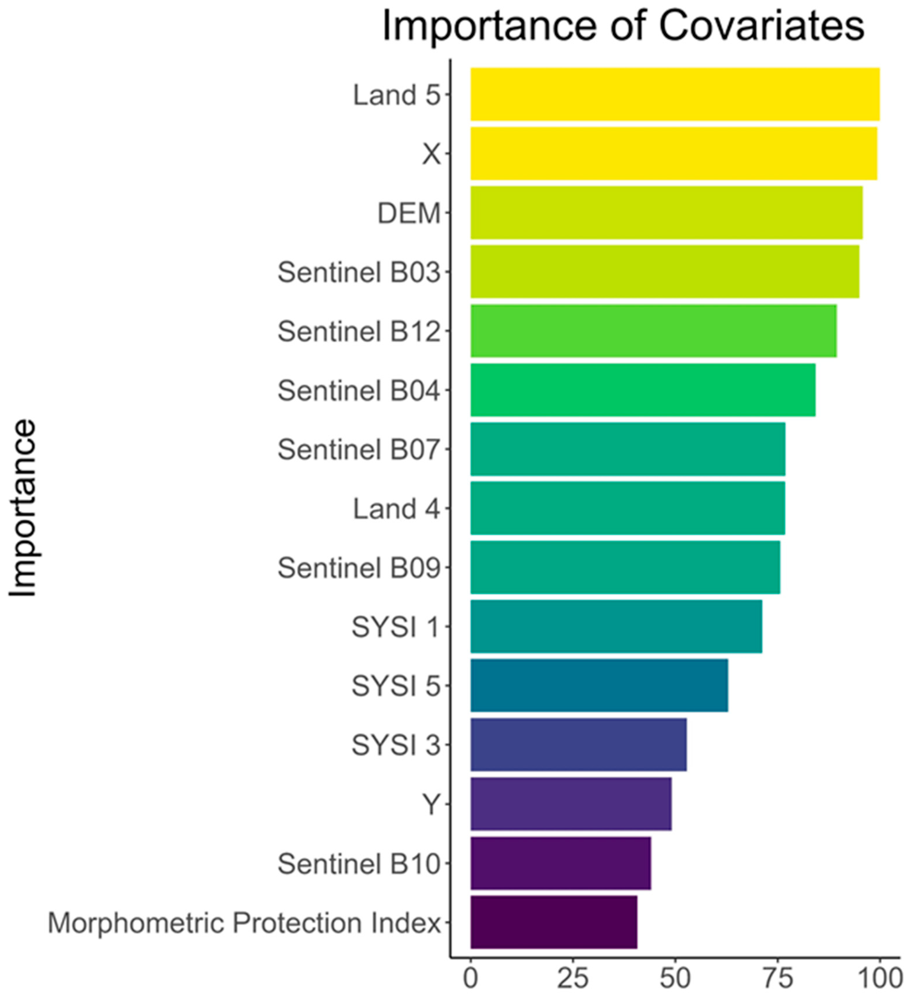
The relatively large number of clusters (5) increased the probability of samples to be classified into an incorrect cluster. Segoni et al. (2012) [42] obtained a standard result confirming that a decrease in the model’s sensitivity positively impact its specificity. This finding aligns with our own results. The satellite bands, SYSI, and geographical coordinates (X and Y) emerged as the most significant variables, contributing to over 50% in the creation of geophysical isoparameters for the SVM algorithm (Figure 4). Although machine learning models initially assign equal weights to all covariates, the availability, resolution, and nature of the input data can influence the calculated relative importance. In this study, RS covariates showed higher importance compared to topographic variables, reflecting a stronger association between RS-derived metrics and the target variable, considering the study area and the sensor characteristics used. However, we recognize that variations in spatial resolution, processing methods, or the inclusion of new environmental variables could alter this importance hierarchy. Future studies exploring a broader range of predictors or different modeling approaches may enhance the understanding of these relationships.
The greater contribution of satellite bands was expected once the soil spectral reflectance is directly related to their attributes, mainly texture (clay and sand content), mineralogy, soil moisture, organic matter content and soil types [48]. In addition, lithology, soil texture, processes and types are directly related to all geophysical variables used and landscapes [21]. The X and Y coordinates demonstrate the effect of the spatial distribution of the samples in the environment. Close samples tend to have similar values of geophysical variables and, therefore, belong to the same class in the modeling process.

3.2. Relationship Between Geophysical-Isoparameters Classes, Lithology and Soil Types

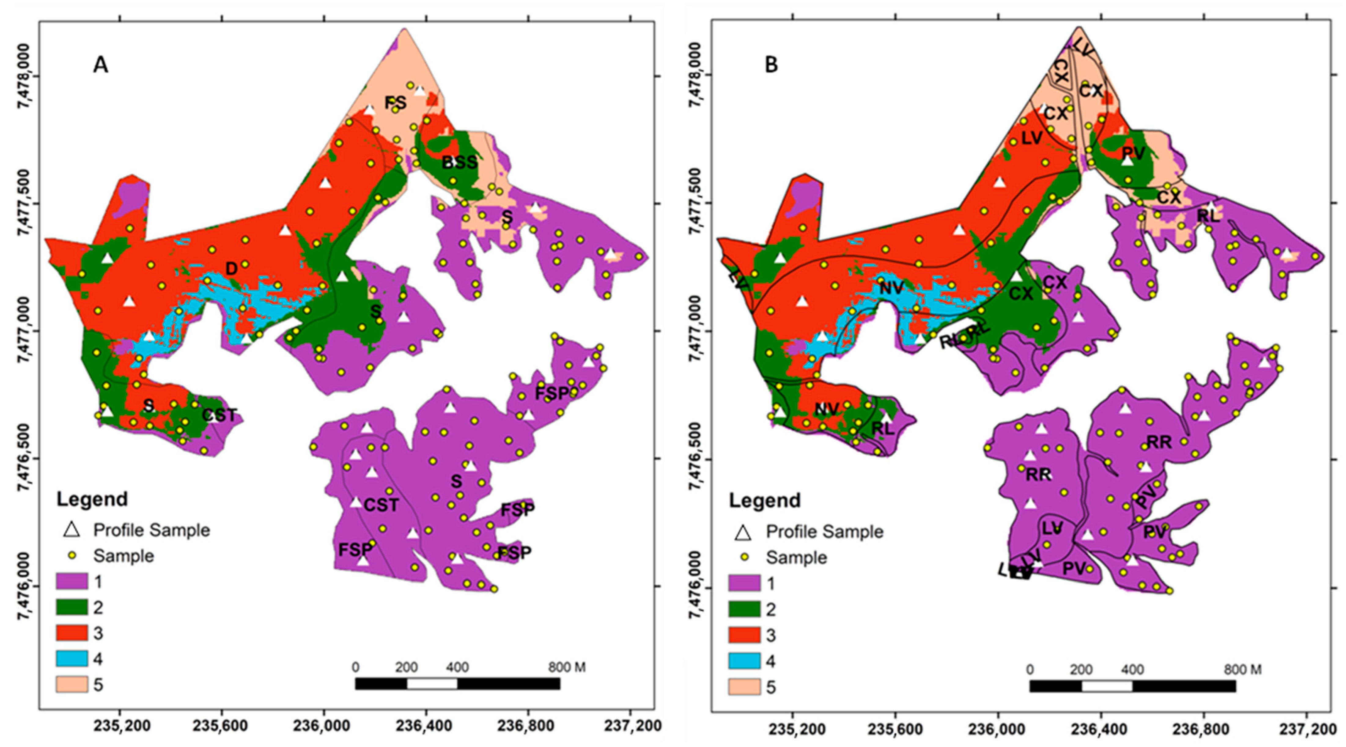
The method efficiently separated geophysical-isoparameters in 1, 3 and 5 classes (Table 6, Figure 5). The main statistical differences between the geophysical variables are observed between classes 1 and 5, and between those and class 3. On the other hand, classes 2 and 4 did not show statistical differences and corresponded to the highest percentage of prediction error (Table 6, Figure 6). The explanation for these statistical differences and separation efficiency of the method is due to the lithological characteristics and to extent, to soils. Class 1 is located on lithology consisting of coarse sedimentary materials (sandstones and siltstones) (Figure 5). These rocks have varied amounts of radionuclides and a low content of ferrimagnetic minerals in the parent material.
Class 3 is located on a system rich in mafic rocks, basalt, and/or associated siltstones (Figure 5), with lower radionuclides contents. On the other hand, Class 3 has higher content of ferrimagnetic minerals in the parent material. Class 5 is located on fluvial sediments (Figure 5) that vary in stratigraphy and, consequently in mineralogical composition and content of radionuclides and ferrimagnetic minerals. Several authors [12,49,50,51] found greater variations in radionuclide content in sedimentary rocks as a function of the type of sediment and degree of weathering.
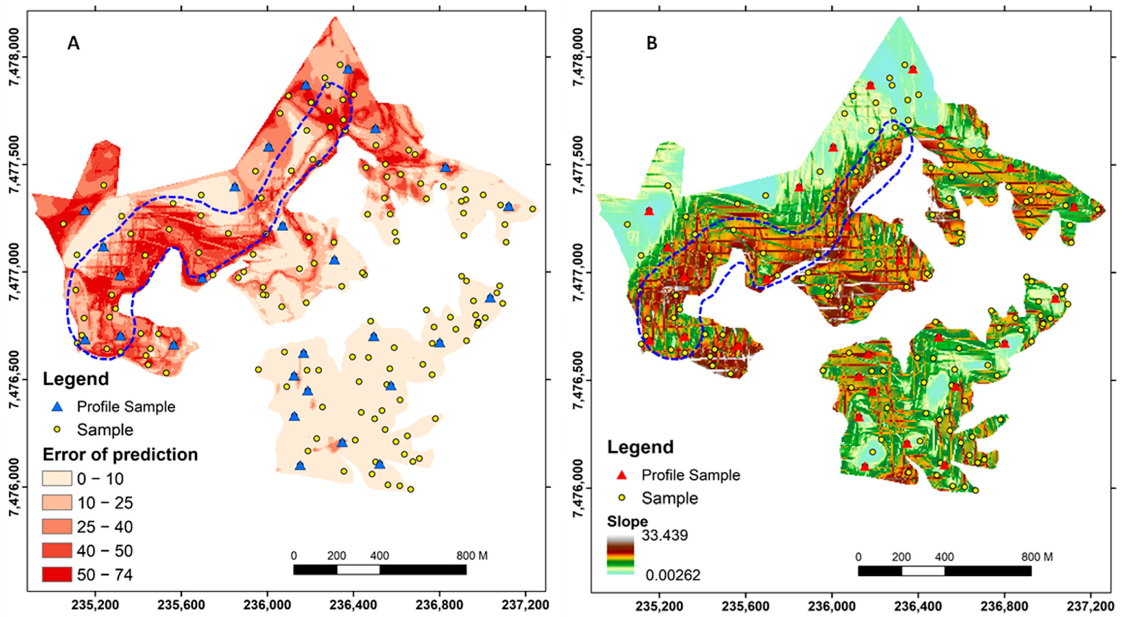
Class 4 is a transition area between two lithological substrates with the influence of basalt and siltstone (Figure 5). Hence, these two classes were not well separated and did not show statistical differences (Table 6, Figure 6). In agreement, Dickson and Scott, (1997) [12] and Mello et al. (2023) [16] demonstrated a decrease in radionuclide content in mafic rocks compared to felsic rocks and a direct relationship between soil κ and the presence of mafic minerals. On the siltstone, the surrounding diabase dike probably increases siltstones in mafic minerals [52], which also affects the intermediate values of ECa. Class 2 is an area of lithological transition and relief (Figure 5A), where mixed colluvial deposition of materials from the upper part of the landscape may have influenced the content of radionuclides and ferrimagnetic minerals, reducing the model performance. The influence of mixing lithologies over another, which affects radionuclide concentration and magnetic susceptibility, was presented and discussed in detail by Mello et al., (2023) [16]. The highest prediction errors in isoparameter classes 2 and 4 occur primarily within lithological transition zones and steep slopes. These environments are characterized by increased mixing of parent materials, variable weathering intensities, and greater heterogeneity in soil mineralogy and texture. Such complexity produces overlapping geophysical signatures that challenge the classification process. For instance, the juxtaposition of mafic and felsic materials introduces sharp contrasts in magnetic mineral content, leading to local fluctuations in soil κ values. Similarly, the redistribution of fine and coarse materials by colluvial processes alters both soil moisture and ionic concentration, directly influencing apparent electrical conductivity (ECa) readings. In gamma-ray spectrometry, radionuclide concentrations (K40, Th, U) tend to vary nonlinearly due to the differential weathering and dilution of source minerals, generating mixed radiometric signals. Consequently, the superposition of these geophysical effects in transitional zones results in signal interference and reduced separability between clusters, which quantitatively explains the higher model errors observed in these areas. These findings emphasize that the transitional zones represent areas of high geophysical complexity where standard clustering methods may underestimate the true variability of the underlying litho-pedological system.
The types of soils in class 1 are constituted sandy/silty soils (Figure 5B), with low cation exchange capacity CEC and low potential to retain radionuclides and to form ferrimagnetic minerals. This is because quartz greatly predominates in the sand fraction, with little iron available forms of secondary ferrimagnetic minerals, such as maghemite. Therefore, the radionuclide content and magnetic susceptibility are lower than class 3.
Class 3 (Figure 5B) constituted by clayey soils (N and LV) with higher clay content, CEC, and higher potential to retain radionuclides [53,54,55]. In addition, there is a predominance of iron-rich minerals that, when weathered, release greater amounts of this element in the system and allow greater formation of ferrimagnetic minerals [56].
Figure 6 also demonstrates a relationship between the largest prediction errors associated with the lower slopes in the landscape. This is because there was greater erosion and deposition of different materials from the higher parts of the landscape, which affects both the radionuclide content and the ECa and k values.

3.3. A Systematic Methodology for Soil Scientists Engaged in Soil-Lithological Surveys

The results obtained in this study demonstrate the feasibility and potential of integrating proximal geophysical sensors, remote sensing data, and machine learning techniques to generate and classify “geophysical-isoparameters.” These quantitative indicators represent coherent combinations of geophysical responses that reflect variations in soil–lithological properties across the landscape. The outcomes validate the central hypothesis proposed in this work, that the integration of field-based geophysical data, satellite imagery, and morphometric attributes can yield consistent and interpretable spatial patterns that serve as a foundation for soil–lithological mapping.
The geophysical-isoparameter concept represents a step forward in transforming raw sensor measurements into meaningful geospatial information. Each isoparameter class reflects a consistent geophysical “fingerprint” that integrates lithological composition, weathering degree, mineralogical content, and soil physical–chemical attributes. Unlike individual sensor variables, which can be noisy or locally variable, geophysical-isoparameters summarize the stable relationships among these datasets, allowing the derivation of reproducible, spatially coherent patterns. Thus, the framework acts as an intermediate layer between primary geophysical data and final pedological–lithological mapping units.
First, we identified optimal locations for soil sampling using augering, data acquisition from three geophysical sensors, and profile evaluation through satellite imagery (Figure 1). These methods were selected due to their low cost, ease of data acquisition, and practicality. Remote and proximal sensing (satellite/SYSI and geophysical sensors) revealed patterns consistent with variations in certain soil attributes, mainly soil color, texture, and moisture [57,58]. In addition, the combined geophysical variables (radiometric, magnetic, and electric) presented differences between soil types, mainly related to soil mineralogy and texture [8]. These attributes are directly related to soil density, structure, and CEC used in land use and management [59,60]. Therefore, combining gamma-ray spectrometry, magnetic susceptibility, and electrical conductivity enhances the knowledge and reduces subjectivity in digital soil classification procedures [8].
The combined geophysical data acquisition should be performed on the topsoil and soil profiles through diagnostic horizons, concomitantly with soil sampling collected for physico-chemical analyses (Figure 1). To quantify and analyze geophysical variables, it is advisable to interpret the patterns of each variable directly on computers through clustering analysis. This approach helps identify differences and similarities between classes (geophysical isoparameters). Adopting this approach makes the process more time-efficient, reduces the need for extensive soil analyses, and decreases reliance on subjective judgments for soil classification [60].
The geophysical–soil dataset provides valuable insights into soil characteristics, particularly mineralogy, texture, and CEC, thereby supporting pedological information. When profiles and surface collection points are adequately described and accurately positioned, integrating proximal and remote sensing data can facilitate the spatialization process and reveal pattern information for extensive areas, as demonstrated in this study using machine learning techniques. The observed surface patterns played a crucial role in delineating soil–lithological mapping units. The clustering of surface information exhibited a clear association with the corresponding soil types and lithology, ultimately leading to the creation of the final map unit.
This integrative approach demonstrates that the proposed “geophysical-isoparameter” framework goes beyond the descriptive nature of conventional soil mapping by transforming qualitative expert interpretation into quantitative, spatially explicit indicators of soil–lithological variability. The methodology enables the identification of consistent geophysical signatures associated with pedogenetic processes and lithological controls, providing a transferable and reproducible foundation for digital soil–lithological surveys. While expert validation remains an essential step, the integration of proximal and remote sensing with machine learning represents a substantial methodological advance, enhancing objectivity, scalability, and reproducibility in soil mapping practices. This work therefore offers a bridge between traditional pedological knowledge and data-driven geophysical analytics, advancing the field toward the next generation of quantitative soil–lithological mapping.
The inclusion of a broad set of terrain attributes may involve some degree of redundancy due to correlations among derived variables (e.g., slope, curvature, and topographic indices). Nevertheless, this comprehensive approach was deliberately adopted to enhance the protocol’s robustness and versatility, enabling the feature selection algorithms to objectively identify the most informative predictors while minimizing subjective or experience-based bias. Rather than compromising interpretability, this design choice reflects a trade-off aimed at ensuring reproducibility and adaptability across different landscapes. Future applications of the protocol may further refine the selection of terrain attributes based on domain expertise, once its overall performance and stability have been validated. In addition, the relatively low contribution of morphometric indices, including the Morphometric Protection Index (MPI) (Figure 4), can be attributed to the geomorphological characteristics of the study area, which is predominantly gentle to moderately undulating. In such landscapes, topographic variation exerts limited control over soil variability compared to spectral and geophysical factors. However, the inclusion of a wide range of morphometric predictors was intentional to guarantee the transferability of the protocol to more complex terrains where relief plays a stronger role in soil formation and distribution. This approach ensures flexibility and objectivity, allowing the model to evaluate the relevance of terrain attributes in a data-driven manner without introducing human bias.
Computational aspects of the proposed protocol: The entire modeling workflow—including data preprocessing, clustering, and classification—was conducted in the R environment (version 4.3.0). The algorithms were implemented using the caret framework, along with the nnet, C50, kknn, randomForest, and kernlab packages. All analyses were performed on a workstation equipped with dual Intel® Xeon® E5-2680 v4 processors (2.4 GHz), 256 GB of DDR4 RAM, and an AMD Radeon RX 580 GPU (8 GB, 2048 stream processors). On average, the data preprocessing and clustering stages required approximately five days (≈120 h) to complete. These computational demands are considered moderate and can be efficiently handled by standard laboratory-grade computers, allowing the protocol to be implemented in most research settings without the need for high-performance computing infrastructure.

4. Conclusions

  • This study introduces a conceptual and operational framework based on “geophysical-isoparameters,” integrating proximal geophysical sensing, remote sensing, and morphometric data to generate quantitative descriptors of soil–lithological variability. The concept represents both a methodological and theoretical advance by transforming qualitative expert interpretation into quantitative, reproducible indicators of soil and lithological variation.
  • The SVM algorithm efficiently classified geophysical-isoparameter classes through the integration of gamma-ray spectrometry, magnetic susceptibility (κ), apparent electrical conductivity (ECa), and satellite imagery. The clustering of geophysical variables successfully captured distinct soil attributes linked to pedogenic and lithological processes, confirming the capacity of multi-source sensing to represent soil–landscape variability.
  • The resulting geophysical-isoparameter maps showed strong correspondence with pedological and lithological units, with prediction errors mainly occurring in transitional zones between lithologies and on steep slopes, areas that are inherently complex for both conventional and digital soil mapping.
  • Satellite bands and SYSI, combined with morphometric variables, were the most influential predictors in the modeling process. Statistical analysis grouped the geophysical variables into two main clusters, while k-means clustering revealed finer distinctions, enhancing mapping detail and interpretability.
  • The proposed protocol establishes a systematic and data-driven approach for delineating soil–lithological units by integrating proximal geophysical data, satellite imagery, and machine learning. This framework reduces subjectivity, improves reproducibility, and provides a consistent quantitative foundation for generating homogeneous classes of geophysical parameters (geophysical-isoparameters).
  • While expert judgment remains essential for final interpretation and validation, the geophysical-isoparameter framework bridges the gap between traditional qualitative surveys and modern data-driven mapping approaches. It fosters interdisciplinary collaboration and advances innovative methodologies for soil–lithology characterization through the combined use of gamma-ray spectrometry, magnetic and electrical surveys, and morphometric data.
  • Future research should focus on refining the integration of additional environmental covariates, testing the protocol in diverse geomorphological and geological settings, and automating class recognition and validation. In doing so, the geophysical-isoparameter framework may serve as a cornerstone for the next generation of objective, quantitative, and transferable soil–lithological mapping methodologies.

Author Contributions

Conceptualization: G.V.V. and D.C.d.M.; methodology: G.V.V. E.I.F.-F.; software: G.V.V.; validation: G.V.V. and D.C.d.M.; formal analysis: G.V.V. and D.C.d.M.; investigation: G.V.V. and D.C.d.M.; resources: R.F., R.B.d.O., M.R.N. and J.A.M.D.; data curation: M.R.F., T.O.F., J.C.Z. and D.F.G.; writing—original draft preparation: D.C.d.M.; writing—review and editing: M.R.F., T.O.F., J.C.Z., D.F.G., H.P.P., M.F.M. and L.V.S.; visualization: H.P.P., M.F.M. and L.V.S.; supervision: J.A.M.D.; project administration, J.A.M.D.; funding acquisition: R.F., and R.B.d.O., M.R.N. and J.A.M.D. All authors have read and agreed to the published version of the manuscript.

Funding

This research received funding from National Council for Scientific and Technological Development (CNPq) for awarding the first author’s scholarship (grant No. 134608/2015-1; grant number 305996/2018-5), and to the São Paulo Research Foundation (FAPESP) for their invaluable support and provision of essential resources to the Laboratory of Remote Sensing Applied to Soils at the “Luiz de Queiroz” College of Agriculture (ESALQ/USP) and, for the scholarship awarded to the first author (project 2024/06285-1), which enabled the completion of this manuscript at another institution (ESALQ/USP).

Data Availability Statement

The original contributions presented in this study are included in the article. Further inquiries can be directed to the corresponding author.

Acknowledgments

We express our sincere appreciation to the National Council for Scientific and Technological Development (CNPq) for awarding the G.V.V., scholarship (grant No. 134608/2015-1; grant number 305996/2018-5), and to the São Paulo Research Foundation (FAPESP) for their invaluable support and provision of essential resources to the Laboratory of Remote Sensing Applied to Soils at the “Luiz de Queiroz” College of Agriculture (ESALQ/USP). We also extend our gratitude to Fundação de Amparo a Pesquisa do Estado de São Paulo (FAPESP) for the scholarship awarded to the second author (project 2024/06285-1), which enabled the completion of this manuscript at another institution (ESALQ/USP). This study was financed in part by the Coordenação de Aperfeiçoamento de Pessoal de Nível Superior—Brazil (CAPES)—Finance Code 001”; This study was financed in part by the Programa de Apoio à Fixação de Jovens Doutores no Brasil (CNPq 168180/2022–7), Fundação Araucária (CP 19/2022—Jovens Doutores). We would like to express our appreciation to the Geotechnologies in Soil Science group (GeoCis) and LabGeo—UFV (Programa de Pós-Graduação em Solos e Nutrição de Plantas—PGSNP) at the Soil Department of the Universidade Federal de Viçosa, Brazil, as well as the Institute of Geosciences at Campinas State University, Brazil, for their valuable support.

Conflicts of Interest

The authors declare that they have no conflicts of interest. The funders had no role in the design of the study; in the collection, analyses, or interpretation of data; in the writing of the manuscript; or in the decision to publish the results.

References

  1. Burrough, P.A. Soil Variability: A Late 20th Century View. Soils Fert. 1993, 56, 529–562. [Google Scholar]
  2. Jenny, H. Factors of Soil Formation; McGraw-Hill: New York, NY, USA, 1941. [Google Scholar]
  3. Jenny, H. Factors of Soil Formation: A System of Quantitative Pedology; Dover Publication: New York, NY, USA, 1994. [Google Scholar]
  4. Keesstra, S.D.; Bouma, J.; Wallinga, J.; Tittonell, P.; Smith, P.; Cerdà, A.; Montanarella, L.; Quinton, J.N.; Pachepsky, Y.; Van Der Putten, W.H. The Significance of Soils and Soil Science towards Realization of the United Nations Sustainable Development Goals. Soil 2016, 2, 111–128. [Google Scholar] [CrossRef]
  5. Montanarella, L.; Pennock, D.J.; McKenzie, N.J.; Badraoui, M.; Chude, V.; Baptista, I.; Mamo, T.; Yemefack, M.; Singh Aulakh, M.; Yagi, K. World’s Soils Are under Threat. Soil 2015, 2, 1263–1272. [Google Scholar] [CrossRef]
  6. Lagacherie, P.; McBratney, A.B. Spatial Soil Information Systems and Spatial Soil Inference Systems: Perspectives for Digital Soil Mapping. Dev. Soil Sci. 2006, 31, 3–22. [Google Scholar]
  7. Stenberg, B. Effects of Soil Sample Pretreatments and Standardised Rewetting as Interacted with Sand Classes on Vis-NIR Predictions of Clay and Soil Organic Carbon. Geoderma 2010, 158, 15–22. [Google Scholar] [CrossRef]
  8. de Mello, D.C.; Veloso, G.V.; de Lana, M.G.; Mello, F.A.d.O.; Poppiel, R.R.; Cabrero, D.R.O.; Di Raimo, L.A.D.L.; Schaefer, C.E.G.R.; Leite, E.P.; Demattê, J.A.M. A New Methodological Framework for Geophysical Sensor Combinations Associated with Machine Learning Algorithms to Understand Soil Attributes. Geosci. Model Dev. 2022, 15, 1219–1246. [Google Scholar] [CrossRef]
  9. de Mello, D.C.; Alexandre Melo Demattê, J.; Alcantara de Oliveira Mello, F.; Roberto Poppiel, R.; ElizabetQuiñonez Silvero, N.; Lucas Safanelli, J.; Barros e Souza, A.; Augusto Di Loreto Di Raimo, L.; Rizzo, R.; Eduarda Bispo Resende, M.; et al. Applied Gamma-Ray Spectrometry for Evaluating Tropical Soil Processes and Attributes. Geoderma 2021, 381, 114736. [Google Scholar] [CrossRef]
  10. Mello, D.; Demattê, J.A.M.; Silvero, N.E.Q.; Di Raimo, L.A.D.L.; Poppiel, R.R.; Mello, F.A.O.; Souza, A.B.; Safanelli, J.L.; Resende, M.E.B.; Rizzo, R. Soil Magnetic Susceptibility and Its Relationship with Naturally Occurring Processes and Soil Attributes in Pedosphere, in a Tropical Environment. Geoderma 2020, 372, 114364. [Google Scholar] [CrossRef]
  11. de Mello, D.C.; Safanelli, J.L.; Poppiel, R.R.; Veloso, G.V.; Cabrero, D.R.O.; Greschuk, L.T.; Mello, F.A.d.O.; Francelino, M.R.; Ker, J.C.; Leite, E.P.; et al. Soil Apparent Electrical Conductivity Survey in Different Pedoenvironments by Geophysical Sensor EM38: A Potential Tool in Pedology and Pedometry Studies. Geocarto Int. 2022, 37, 13057–13078. [Google Scholar] [CrossRef]
  12. Dickson, B.L.; Scott, K.M. Interpretation of Aerial Gamma-Ray Surveys—Adding the Geochemical Factors. AGSO J. Aust. Geol. Geophys. 1997, 17, 187–200. [Google Scholar]
  13. Rochette, P.; Jackson, M.; Aubourg, C. Rock Magnetism Andn the Interpretation of Magnetic Susceptibility. Rev. Geophys. 1992, 30, 209–226. [Google Scholar] [CrossRef]
  14. Corwin, D.L.; Lesch, S.M. Application of Soil Electrical Conductivity to Precision Agriculture: Theory, Principles, and Guidelines. Agron. J. 2003, 95, 455–471. [Google Scholar] [CrossRef]
  15. Mello, D.C.; Veloso, G.V.; Moquedace, C.M.; de Angeli Oliveira, I.; de Oliveira, F.S.; Gomes, L.C.; de Souza, J.J.L.L.; Francelino, M.R.; Fernandes-Filho, E.I.; Schaefer, C.E.G.R.; et al. Radiometric and Magnetic Susceptibility Characterization of Soil Profiles: Geophysical Data and Their Relationship with Antarctic Periglacial Processes, Pedogenesis, and Lithology. CATENA 2023, 232, 107427. [Google Scholar] [CrossRef]
  16. Mello, D.C.; Vieira, G.; Marques, C.; De Angeli, I.; Soares, F.; Oliveira, D.; Demattê, M. Chemical Weathering Detection in the Periglacial Landscapes of Maritime Antarctica: New Approach Using Geophysical Sensors, Topographic Variables and Machine Learning Algorithms. Geoderma 2023, 438, 116615. [Google Scholar] [CrossRef]
  17. de Mello, D.C.; Ferreira, T.O.; Veloso, G.V.; de Lana, M.G.; de Oliveira Mello, F.A.; Di Raimo, L.A.D.L.; Cabrero, D.R.O.; de Souza, J.J.L.L.; Fernandes-Filho, E.I.; Francelino, M.R. Digital Mapping of Soil Weathering Using Field Geophysical Sensor Data Coupled with Covariates and Machine Learning. J. S. Am. Earth Sci. 2023, 128, 104449. [Google Scholar] [CrossRef]
  18. Rentschler, T.; Werban, U.; Ahner, M.; Behrens, T.; Gries, P.; Scholten, T.; Teuber, S.; Schmidt, K. 3D Mapping of Soil Organic Carbon Content and Soil Moisture with Multiple Geophysical Sensors and Machine Learning. Vadose Zone J. 2020, 19, e20062. [Google Scholar] [CrossRef]
  19. Luiz do Carmo Leal, A.; da Costa Lauria, D.; Ribeiro, F.C.A.; Viglio, E.P.; Franzen, M.; de Albuquerque Medeiros Lima, E. Spatial Distributions of Natural Radionuclides in Soils of the State of Pernambuco, Brazil: Influence of Bedrocks, Soils Types and Climates. J. Environ. Radioact. 2020, 211, 106046. [Google Scholar] [CrossRef]
  20. Ribeiro, F.C.A.; Lauria, D.d.C.; do Rio, M.A.P.; da Cunha, F.G.; de Oliveira Sousa, W.; de Albuquerque Medeiros Lima, E.; Franzen, M. Mapping Soil Radioactivity in the Fernando de Noronha Archipelago, Brazil. J. Radioanal. Nucl. Chem. 2017, 311, 577–587. [Google Scholar] [CrossRef]
  21. Ribeiro, F.C.A.; Silva, J.I.R.; Lima, E.S.A.; do Amaral Sobrinho, N.M.B.; Perez, D.V.; Lauria, D.C. Natural Radioactivity in Soils of the State of Rio de Janeiro (Brazil): Radiological Characterization and Relationships to Geological Formation, Soil Types and Soil Properties. J. Environ. Radioact. 2018, 182, 34–43. [Google Scholar] [CrossRef]
  22. Silva, F.M.; Silva, S.H.G.; Andrade, R.; Coblinski, J.A.; Inda, A.V.; Frosi, G.; Lima, S.d.S.F.; de Menezes, M.D.; Tavares, T.R.; Guilherme, L.R.G.; et al. Proximal Sensors for Modeling Clay Mineralogy and Characterization of Soil Textural Fractions Developed from Contrasting Parent Materials. CATENA 2024, 241, 108053. [Google Scholar] [CrossRef]
  23. Ramos, P.V.; Dalmolin, R.S.D.; Marques Júnior, J.; Siqueira, D.S.; De Almeida, J.A.; Moura-Bueno, J.M. Magnetic Susceptibility of Soil to Differentiate Soil Environments in Southern Brazil. Rev. Bras. Cienc. Do Solo 2017, 41, 1–13. [Google Scholar] [CrossRef]
  24. Farzamian, M.; Monteiro Santos, F.A.; Khalil, M.A. Application of EM38 and ERT Methods in Estimation of Saturated Hydraulic Conductivity in Unsaturated Soil. J. Appl. Geophys. 2015, 112, 175–189. [Google Scholar] [CrossRef]
  25. Narjary, B.; Meena, M.D.; Kumar, S.; Kamra, S.K.; Sharma, D.K.; Triantafilis, J. Digital Mapping of Soil Salinity at Various Depths Using an EM38. Soil Use Manag. 2019, 35, 232–244. [Google Scholar] [CrossRef]
  26. Bonfatti, B.R.; Demattê, J.A.M.; Marques, K.P.P.; Poppiel, R.R.; Rizzo, R.; Mendes, W.d.S.; Silvero, N.E.Q.; Safanelli, J.L. Digital Mapping of Soil Parent Material in a Heterogeneous Tropical Area. Geomorphology 2020, 367, 107305. [Google Scholar] [CrossRef]
  27. Alvares, C.A.; Stape, J.L.; Sentelhas, P.C.; De Moraes Gonçalves, J.L.; Sparovek, G. Köppen’s Climate Classification Map for Brazil. Meteorol. Z. 2013, 22, 711–728. [Google Scholar] [CrossRef]
  28. Georesults. Terraplus KT-10 v2 User Manual 2021, User’s Guide Ver. 2.1; Georesults: Cumming, GA, USA, 2021. [Google Scholar]
  29. de Sousa, G.P.B.; Bellinaso, H.; Rosas, J.T.F.; de Mello, D.C.; Rosin, N.A.; Amorim, M.T.A.; dos Anjos Bartsch, B.; Cardoso, M.C.; Mallah, S.; Francelino, M.R.; et al. Assessing Soil Degradation in Brazilian Agriculture by a Remote Sensing Approach to Monitor Bare Soil Frequency: Impact on Soil Carbon. Soil Adv. 2024, 2, 100011. [Google Scholar] [CrossRef]
  30. Demattê, J.A.M.; Fongaro, C.T.; Rizzo, R.; Safanelli, J.L. Geospatial Soil Sensing System (GEOS3): A Powerful Data Mining Procedure to Retrieve Soil Spectral Reflectance from Satellite Images. Remote Sens. Environ. 2018, 212, 161–175. [Google Scholar] [CrossRef]
  31. Hijmans, R.J.; Van Etten, J. Raster: Geographic Data Analysis and Modeling; R Package Version 2.5-8; R Core Team: Vienna, Austria, 2016. [Google Scholar]
  32. R Core Team. R: A Language and Environment for Statistical Computing; R Core Team: Vienna, Austria, 2023. [Google Scholar]
  33. Matsuura, D.; Chounan, Y.; Sugahara, Y.; Takeda, Y. Wearable Working Assist Mechanism for Hemiplegics Capable of Changing Step Length and Walking Direction. In New Trends in Medical and Service Robotics; Springer: Berlin/Heidelberg, Germany, 2019; pp. 126–133. [Google Scholar]
  34. Halkidi, M.; Vazirgiannis, M.; Batistakis, Y. Quality Scheme Assessment in the Clustering Process. In Proceedings of the Principles of Data Mining and Knowledge Discovery: 4th European Conference, PKDD 2000, Lyon, France, 13–16 September 2000; Proceedings 4. Springer: Berlin/Heidelberg, Germany, 2000; pp. 265–276. [Google Scholar]
  35. Charrad, M.; Ghazzali, N.; Boiteau, V.; Niknafs, A. NbClust: An R Package for Determining the Relevant Number of Clusters in a Data Set. J. Stat. Softw. 2014, 61, 1–36. [Google Scholar] [CrossRef]
  36. Kuhn, M. Building predictive models in R using the caret package. J. Stat. Softw. 2008, 28, 1–26. [Google Scholar] [CrossRef]
  37. Meng, E.; Huang, S.; Huang, Q.; Fang, W.; Wu, L.; Wang, L. A Robust Method for Non-Stationary Streamflow Prediction Based on Improved EMD-SVM Model. J. Hydrol. 2019, 568, 462–478. [Google Scholar] [CrossRef]
  38. Deka, P.C. Support Vector Machine Applications in the Field of Hydrology: A Review. Appl. Soft Comput. 2014, 19, 372–386. [Google Scholar] [CrossRef]
  39. Gomes, L.C.; Faria, R.M.; de Souza, E.; Veloso, G.V.; Ernesto, C.; Schaefer, G.R.; Inácio, E.; Filho, F. Modelling and Mapping Soil Organic Carbon Stocks in Brazil. Geoderma 2019, 340, 337–350. [Google Scholar] [CrossRef]
  40. Zar, J.H. Biostatistical Analysis; Prentice Hall: Upper Saddle River, NJ, USA, 1999. [Google Scholar]
  41. Islam, F.; Ahmad, M.N.; Janjuhah, H.T.; Ullah, M.; Islam, I.U.; Kontakiotis, G.; Skilodimou, H.D.; Bathrellos, G.D. Modelling and Mapping of Soil Erosion Susceptibility of Murree, Sub-Himalayas Using GIS and RS-Based Models. Appl. Sci. 2022, 12, 12211. [Google Scholar] [CrossRef]
  42. Segoni, S.; Rossi, G.; Catani, F. Improving Basin Scale Shallow Landslide Modelling Using Reliable Soil Thickness Maps. Nat. Hazards 2012, 61, 85–101. [Google Scholar] [CrossRef]
  43. Barman, U.; Choudhury, R.D. Soil Texture Classification Using Multi Class Support Vector Machine. Inf. Process. Agric. 2020, 7, 318–332. [Google Scholar] [CrossRef]
  44. Al Masmoudi, Y.; Bouslihim, Y.; Doumali, K.; Hssaini, L.; Ibno Namr, K. Use of Machine Learning in Moroccan Soil Fertility Prediction as an Alternative to Laborious Analyses. Model. Earth Syst. Environ. 2021, 8, 3707–3717. [Google Scholar] [CrossRef]
  45. Azadnia, R.; Jahanbakhshi, A.; Rashidi, S. Developing an Automated Monitoring System for Fast and Accurate Prediction of Soil Texture Using an Image-Based Deep Learning Network and Machine Vision System. Measurement 2022, 190, 110669. [Google Scholar] [CrossRef]
  46. Nguyen, T.T.; Pham, T.D.; Nguyen, C.T.; Delfos, J.; Archibald, R.; Dang, K.B.; Hoang, N.B.; Guo, W.; Ngo, H.H. A Novel Intelligence Approach Based Active and Ensemble Learning for Agricultural Soil Organic Carbon Prediction Using Multispectral and SAR Data Fusion. Sci. Total Environ. 2022, 804, 150187. [Google Scholar] [CrossRef]
  47. Ben-Dor, E.; Taylor, R.G.; Hill, J.; Demattê, J.A.M.; Whiting, M.L.; Chabrillat, S.; Sommer, S. Imaging Spectrometry for Soil Applications. Adv. Agron. 2008, 97, 321–392. [Google Scholar]
  48. Arnedo, M.A.; Rubiano, J.G.; Alonso, H.; Tejera, A.; González, A.; González, J.; Gil, J.M.; Rodríguez, R.; Martel, P.; Bolivar, J.P. Mapping Natural Radioactivity of Soils in the Eastern Canary Islands. J. Environ. Radioact. 2017, 166, 242–258. [Google Scholar] [CrossRef]
  49. Boyle, R.W. Geochemical Prospecting for Thorium and Uranium Deposits; Elsevier Scientific Publishing Company: Amsterdam, The Netherlands, 1982. [Google Scholar]
  50. Wilford, J.R.; Bierwirth, P.N.; Craig, M.A. Application of Airborne Gamma-Ray Spectrometry in Soil/Regolith Mapping and Applied Geomorphology. AGSO J. Aust. Geol. Geophys. 1997, 17, 201–216. [Google Scholar]
  51. Sawyer, E.W. The Influence of Source Rock Type, Chemical Weathering and Sorting on the Geochemistry of Clastic Sediments from the Quetico Metasedimentary Belt, Superior Province, Canada. Chem. Geol. 1986, 55, 77–95. [Google Scholar] [CrossRef]
  52. Dierke, C.; Werban, U. Relationships between Gamma-Ray Data and Soil Properties at an Agricultural Test Site. Geoderma 2013, 199, 90–98. [Google Scholar] [CrossRef]
  53. Herrmann, L.; Schuler, U.; Rangubpit, W.; Erbe, P.; Surinkum, A.; Zarei, M.; Stahr, K. The Potential of Gamma-Ray Spectrometry for Soil Mapping. In Proceedings of the 19th World Congress of Soil Science, Brisbane, Australia, 1–6 August 2010; pp. 117–120. [Google Scholar]
  54. Wilford, J.; Minty, B. The Use of Airborne Gamma-Ray Imagery for Mapping Soils and Understanding Landscape Processes. Dev. Soil Sci. 2006, 31, 207–610. [Google Scholar]
  55. Lourenço, A.M.; Sequeira, E.; Sant’Ovaia, H.; Gomes, C.R. Magnetic, Geochemical and Pedological Characterisation of Soil Profiles from Different Environments and Geological Backgrounds near Coimbra, Portugal. Geoderma 2014, 213, 408–418. [Google Scholar] [CrossRef]
  56. Fabre, S.; Briottet, X.; Lesaignoux, A. Estimation of Soil Moisture Content from the Spectral Reflectance of Bare Soils in the 0.4–2.5 Μm Domain. Sensors 2015, 15, 3262–3281. [Google Scholar] [CrossRef]
  57. Mohamed, E.S.; Saleh, A.M.; Belal, A.B.; Gad, A. Application of Near-Infrared Reflectance for Quantitative Assessment of Soil Properties. Egypt. J. Remote Sens. Space Sci. 2018, 21, 1–14. [Google Scholar] [CrossRef]
  58. Haile, G.; Itanna, F.; Teklu, B.; Agegnehu, G. Variation in Soil Properties under Different Land Use Types Managed by Smallholder Farmers in Central Ethiopia. Sustain. Environ. 2022, 8, 2093058. [Google Scholar] [CrossRef]
  59. Batista, R.F.; Reichert, J.M.; Holthusen, D.; Batistão, A.C.; Daher, M.; Schünemann, A.L.; Fernandes Filho, E.I.; Schaefer, C.E.G.R.; Francelino, M.R. Freeze–thaw Cycles Affecting Rheological Properties of Antarctic Soils. Geoderma 2022, 428, 116220. [Google Scholar] [CrossRef]
  60. Odgers, N.P.; McBratney, A.B.; Minasny, B. Bottom-up Digital Soil Mapping. I. Soil Layer Classes. Geoderma 2011, 163, 38–44. [Google Scholar] [CrossRef]
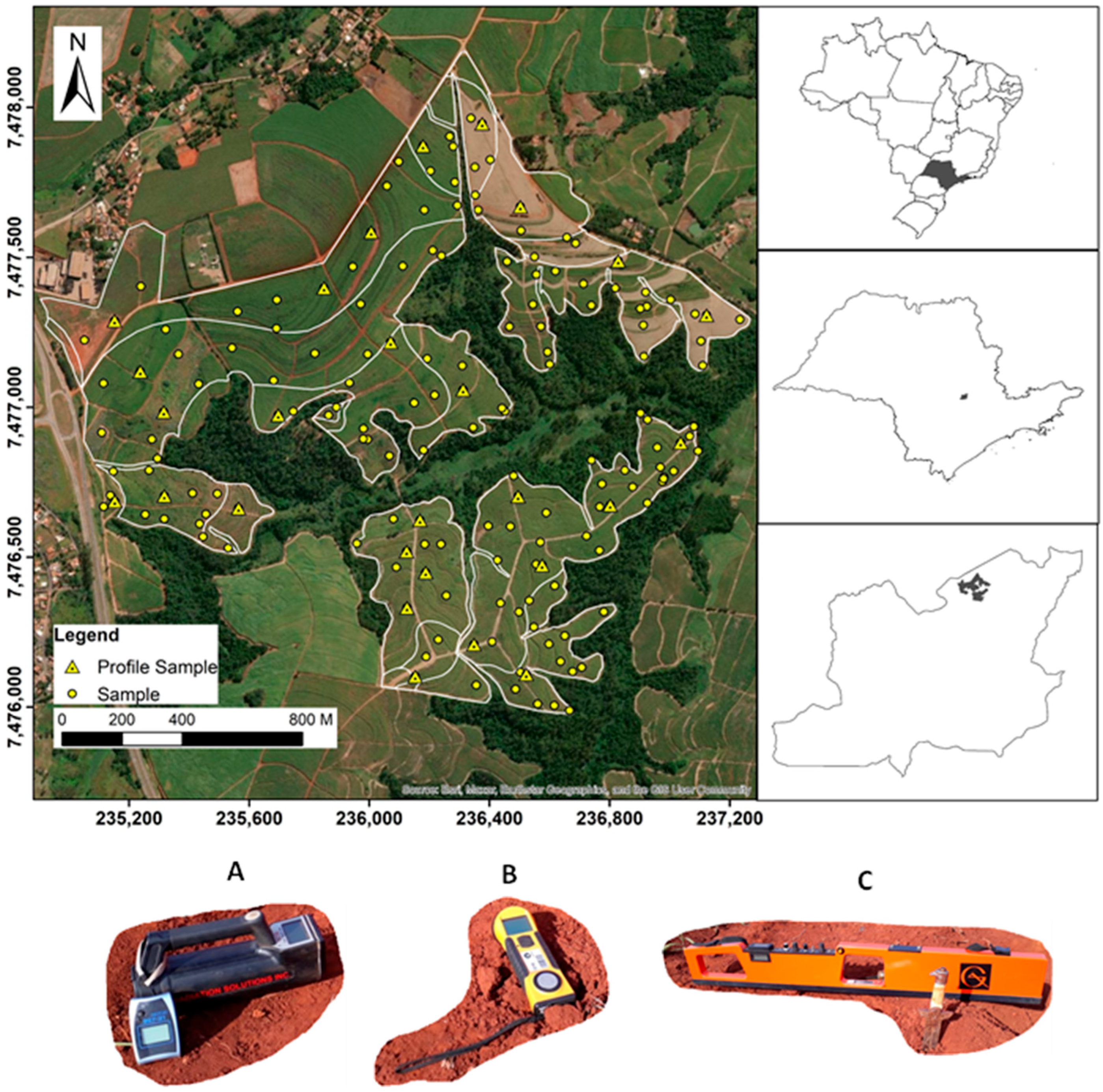
Figure 1. Study site: (A): Gamma-ray spectrometer RS-230; (B): Magnetic susceptibilimeter KT-10 Terraplus; (C): Conductivimeter EM38-Geonics. Note: Soil classes - CX: Haplic Cambisol; LV: Rhodic Ferralsol; NV: Rhodic Nitisol; PV: Rhodic Lixisols; RL: Lithic Leptosol; RR: Dystric Regosol.
Soilsystems 09 00124 g001
Figure 2. (A) Lithology: BSS: basalt–siltite system; CST: sandstone tubarão; D: Diabase; FS: Fluvial sediments; FSP: sandstone pirambóia; S: siltite; (B) Soil classes: CX: Haplic Cambisol; LV: Rhodic Ferralsol; NV: Rhodic Nitisol; PV: Rhodic Lixisols; RL: Lithic Leptosol; RQ: Dystric Arenosol; RR: Dystric Regosol.
Soilsystems 09 00124 g002
Figure 3. Methodological flowchart showing the sequence of methodologies applied for geophysical-isoparameters final map.
Soilsystems 09 00124 g003
Figure 4. Importance of covariate of predictors. The “viridis” color scale indicates the relative importance of the covariates along the axis, where blue tones denote lower importance, and yellow tones denote higher importance.
Soilsystems 09 00124 g004
Figure 5. (A): Geophysical isoparameters classes and lithology; (B): Geophysical isoparameters classes and soil types: D: Diabase: BSS: Basalt–Siltite System; S: Siltite: FS: Fluvial Sediments: FSP: Fine Sandstone Pirambóia; CST: Coarse-Sandstone Tubarão; LV: Rhodic Ferralsol; NV: Rhodic Nitisol; RR: Regosol; RL: Leptosol; CX: Eutric Cambisol; PV: Rhodic Lixisol.
Soilsystems 09 00124 g005
Figure 6. (A): Error of prediction; (B): Slope. The dashed lines in blue indicate a relationship between the highest prediction errors and the highest slope of the terrain.
Soilsystems 09 00124 g006
Table 1. Geophysical parameters used in clusterization (input data). All parameters were generated from the original data and calculated by equations.
Geophysical DataAbbreviationsBrief Description
Equivalent uraniumeUEstimated concentrations of uranium, derived indirectly by measuring the gamma radiation emitted by its daughter products (Bi-214 for uranium-238)
Equivalent thoriumeThEstimated concentrations of thorium, derived indirectly by measuring the gamma radiation emitted by its daughter products (Tl-208 for thorium-232).
Potassium 40K40refers to the estimated concentration of potassium derived indirectly by measuring the gamma radiation emitted by the naturally occurring radioactive isotope potassium-40 (K-40).
Soil apparent electric conductivityECathe ability of the soil to conduct electrical current
Soil magnetic susceptibilityκthe degree to which soils can be magnetized
Ratio equivalent thorium/potassium 40eTh/K40Indicates the relative abundance of thorium compared to potassium-bearing minerals; useful for assessing weathering intensity and mineralogical variations in soils.
Ratio equivalent uranium/potassium 40eU/K40Reflects the enrichment or depletion of uranium relative to potassium; helps infer pedogeochemical processes such as leaching, mineral alteration, or secondary uranium mobility.
Ratio equivalent uranium + equivalent thorium/potassium 40(eU + eTh)/K40Measures the combined relative enrichment of heavy radioactive elements (U + Th) compared to potassium; often used as an index of soil or rock evolution and weathering degree.
Ratio potassium 40/soil magnetic susceptibilityK40Relates the potassium content to the concentration of magnetic minerals; provides insight into soil formation processes and the balance between mineral weathering and ferrimagnetic mineral input.
Ratio equivalent thorium/soil magnetic susceptibilityeTh/κIndicates thorium enrichment relative to magnetic mineral content; useful for tracing sediment sources and differentiating soil types.
Ratio equivalent uranium/soil magnetic susceptibilityeU/κAssesses uranium distribution relative to ferrimagnetic minerals; can reveal soil-forming processes, pollution sources, or geochemical anomalies.
Ratio soil magnetic susceptibility/Soil apparent electrical conductivityκ/ECaCombines magnetic and electrical soil properties; helps differentiate between soil texture, moisture conditions, and mineralogical composition.
Table 2. Description of satellite bands used from Sentinel 2 and Landsat 8.
Sentinel 2Landsat 8
BandWavelength Range (μm)Center Wavelength (μm)FWHM (nm)BandWavelength Range (μm)Center Wavelength (μm)FWHM (nm)
Band 2 (Blue)0.45–0.520.48570Band 1 (Coastal/Aerosol)0.43–0.450.4430
Band 3 (Green)0.54–0.580.5670Band 2 (Blue)0.45–0.510.4860
Band 4 (Red)0.65–0.680.66530Band 3 (Green)0.53–0.590.5660
Band 5 (Red-edge)0.69–0.720.70515Band 4 (Red)0.64–0.670.65530
Band 6 (Red-edge)0.73–0.750.7415Band 5 (NIR)0.85–0.880.86530
Band 7 (Red-edge)0.77–0.790.7820Band 6 (SWIR-1)1.57–1.651.6180
Band 8 (NIR)0.78–0.890.835106Band 7 (SWIR-2)2.11–2.292.20180
Band 8A (NIR narrow)0.85–0.870.8620Band 8 (Panchromatic)0.50–0.680.59180
Band 9 (Water vapour)0.93–0.950.9420Band 10 (TIR-1)10.6–11.1910.895590
Band 9 (Cirrus/SWIR-1)1.36–1.391.37520Band 11 (TIR-2)11.5–12.5112.0051010
Band 10 (SWIR-1)1.57–1.651.6190----
Band 11 (SWIR-2)2.11–2.292.20180----
Table 3. Terrain attributes generated from the digital elevation model.
Terrain AttributesAbbreviationsBrief Description
AspectASSlope orientation
Convergence indexCIConvergence/divergence index in relation to runoff
Cross sectional curvatureCSCMeasures the curvature perpendicular to the down slope direction
Diurnal anisotropic heatingDAHContinuous measurement of exposure dependent energy
Flow line curvatureFLCRepresents the projection of a gradient line to a horizontal plane
General curvatureGCThe combination of both plan and profile curvatures
HillHIAnalytical hill shading
Hill indexHIINDEXAnalytical index hill shading
Longitudinal curvatureLCMeasures the curvature in the down slope direction
Mass balance indexMBIBalance index between erosion and deposition
Maximal curvatureMAXCMaximum curvature in local normal section
Mid-slope positionMSPRepresents the distance from the top to the valley, ranging from 0 to 1
Minimal curvatureMINCMinimum curvature for local normal section
Multiresolution index of ridge top flatnessMRRTFIndicates flat positions in high altitude areas
Multiresolution index of valley bottom flatnessMRVBFIndicates flat surfaces at bottom of valley
Normalized heightNHVertical distance between base and ridge of normalized slope
Plan curvaturePLANCDescribed as the curvature of the hypothetical contour line passing through a specific cell
Profile curvaturePROCDescribes surface curvature in the direction of the steepest incline
Real surface areaRSAActual calculation of cell area
SlopeSRepresents local angular slope
Slope heightSHVertical distance between base and ridge of slope
Slope IndexSIRepresents a local angular slope index
Standardized heightSTANHVertical distance between base and standardized slope index
Surface specific pointsSSPIndicates differences between specific surface shift points
Tangential curvatureTANCMeasured in the normal plane in a direction perpendicular to the gradient
Terrain ruggedness indexTRIQuantitative index of topography heterogeneity
Terrain surface convexityTSCRatio of the number of cells that have positive curvature to the number of all valid cells within a specified search radius
Terrain surface textureTSTSplits surface texture into 8, 12, or 16 classes
Total curvatureTCGeneral measure of surface curvature
Topographic position indexTPIDifference between a point elevation with surrounding elevation
Valley depthVDCalculation of vertical distance at drainage base level
ValleyVACalculation fuzzy valley using the Top Hat approach
Valley IndexVACalculation fuzzy valley index using the Top Hat approach
Vector ruggedness measureVRMMeasures the variation in terrain roughness
Topographic wetness indexTWIDescribes the tendency of each cell to accumulate water as a function of relief
Table 4. Removed Covariates.
No.Covariate NameNo.Covariate Name
s1land_111Sentinel_B11
2land_212SYSI_2
3land_313SYSI_4
4land_614SYSI_6
5land_715curv_cross sectional
6Sentinel_B0216curv_plan
7Sentinel_B0517curv_profile
8Sentinel_B0618mass_balance_index
9Sentinel_B0819terrain_ruggedness_index
10Sentinel_B8A
Table 5. Model’s performance in terms of F1-Score, accuracy, kappa, sensitivity, and specificity.
Parameter of PerformanceAlgorithms
avNNetC5.0kknnRFSVM
F-1 Score0.495 a 0.467 a0.473 a 0.473 a0.497 a
Accuracy0.547 b0.514 b0.549 a0.543 b0.565 a
Kappa0.351 ab0.318 b0.367 a0367 b 0.37 ab
Sensitivity0.421 a0.418 a0.442 a0.435 a0.430 a
Specificity0.875 b0.866 b0.879 b0.875 ab0.879 ab
avNNet: Model Averaged Neural Network; C5.0: Classificatory 5.0; kknn: k-Nearest Neighbors; RF: Random Forest: SVM: Support Vector Machine. Different letters indicate significant differences among the Parameters of Performance at p ≤ 0.05, according to the Kruskal–Wallis test followed by Dunn’s post hoc test.
Table 6. Statistical analysis for the five clusters, for the geophysical isoparameters by the Kruskal–Wallis.
Geophysical
Isoparameters Classes
eU (ppm)eTh (ppm)K40 (%)κ (m3 kg−1)ECa (mSm−1)Th/KU/KU + (K/Th)K. κTh. κU. κκ. ECa
13.44 a13.02 ab0.98 a2.47 a25.67 a17.32 a5.13 a22.44 a1.75 a19.86 a5.21 a0.12 a
23.93 ab11.34 ab0.49 b22.36 b−12.83 b134.70 b49.83 b184.56 b0.17 b2.90 b1.07 bc−0.32 ab
33.73 a10.83 a0.16 b32.2 b−27.48 b645.78 c239.84 b885.64 b0.18 b2.83 b0.77 b−0.55 b
42.98 a9.40 ab0.12 b50.18 b−47.25 ab75.08 bc22.58 b97.65 b0.2 b0.20 b0.08 b−0.48 ab
55.59 b14.30 b0.31 b5.55 ab9.93 ab275.72 bc140.29 b416.01 b9.44 ab9.44 ab3.15 ac−0.19 a
Notes: Different letters indicate significant differences among the five clusters, for the geophysical isoparameters at p ≤ 0.05, according to the Kruskal–Wallis test followed by Dunn’s post hoc test.
Disclaimer/Publisher’s Note: The statements, opinions and data contained in all publications are solely those of the individual author(s) and contributor(s) and not of MDPI and/or the editor(s). MDPI and/or the editor(s) disclaim responsibility for any injury to people or property resulting from any ideas, methods, instructions or products referred to in the content.