Soil Mapping of Small Fields with Limited Number of Samples by Coupling EMI and NIR Spectroscopy

Abstract

Precision agriculture relies on highly detailed soil maps to optimize resource use. Proximal sensing methods, such as EMI, require a certain number of soil samples and laboratory analysis to interpolate the characteristics of the soil. NIR diffuse reflectance spectroscopy offers a rapid, low-cost alternative that increases datapoints and map accuracy. This study tests and optimizes a methodology for high-detail soil mapping in a 2.5 ha hazelnut grove in Grosseto, Southern Tuscany, Italy, using both EMI sensors (GF Mini Explorer, Brno, Czech Republic) and a handheld NIR spectrometer (Neospectra Scanner, Si-Ware Systems, Menlo Park, CA, USA). In addition to two profiles selected by clustering, another 35 topsoil augerings (0–30 cm) were added. Laboratory analyses were performed on only five samples (two profiles + three samples from the augerings). Partial least square regression (PLSR) with a national spectral library, augmented by the five local samples, predicted clay, sand, organic carbon (SOC), total nitrogen (TN), and cation exchange capacity (CEC). The 37 predicted datapoints were used for spatial interpolation, using the ECa map, elevation, and DEM derivatives as covariates. Kriging with external drift (KED) was used to spatialize the results. The errors of the predictive maps were calculated using five additional validation points analyzed by conventional methods. The validation showed good accuracy of the predictive maps, particularly for SOC and TN.

1. Introduction

Knowledge of soil spatial variability at the field scale is fundamental for site-specific agriculture [1]. Traditional soil sampling and laboratory analysis methods provide detailed information about soil at specific locations but are often limited in number and spatial coverage. At the field scale, mapping the spatial variability of soil properties using only traditional point methods is expensive, impractical, and is usually characterized by low spatial accuracy [2]. In the last two decades, proximal soil sensing (PSS) methods have been widely used to fill the data gap between sampling points and suitable high-detail soil maps [3,4,5,6,7,8].

Among PSS methods, electromagnetic induction (EMI) sensing is one of the most widely used methods to map soil spatial variability, and it has also found several agronomic applications by private companies and consultants supporting precision agriculture [9,10,11]. The success of this PSS technique has been mainly due to its speed of measurement, its relatively low cost, and the volume of the soil investigated [12]. The possibility to use mobile EMI sensors, synchronized with GPS positioning data, allows continuous measurements to be made and a large amount of spatial data to be obtained. EMI sensors measure the apparent electrical conductivity (ECa) of the soil without direct contact with the surface. ECa is an indirect indicator of several physical and hydrological parameters of the soil, as well as of eventual salinity [13]. All these soil parameters influence the electrical conductance pathways into the soil [14]. In non-saline soils, the factors that mostly influence ECa are clay content and mineralogy, cation exchange capacity (CEC), coarse fragments, soil porosity, and moisture content [12,15,16]. Since ECa is influenced by numerous soil properties, an accurate interpretation of the collected data is necessary to understand how the spatial variability of ECa is correlated with the spatial variability of individual soil properties [15]. The direct correlation between ECa and a single soil property is mainly site-specific and sometimes subjected to temporal variation, as in the case of soil moisture [17]. Sometimes, the correlation between ECa and a single soil property can be very low, because the spatial variation of ECa is driven by multiple soil parameters, both in the topsoil and in the subsoil. Therefore, the calibration of inference models to predict soil properties, using ECa maps as covariates, must be based on targeted soil observation and analysis, and, sometimes, the inference model may be unreliable [16]. A calibration sampling design that covers the entire study area and its spatial variability is needed [4]. On the other hand, field-scale soil mapping must be economically sustainable, to be performed by consultants and professional users. For commercial use of proximal soil sensing and mapping, typically no more than one or two samples per hectare can be collected and analyzed by laboratory methods [9]. This sampling frequency can be a major problem when the surveyed area is only a few hectares wide, making the proximal sensing method unviable for small farms.

The information collected from the EMI sensor can be combined with other sources of information, both proximal and remote, to increase the reliability of the soil properties estimation [18,19]. Diffuse reflectance spectroscopy (DRS) in the visible (VIS) and/or near-infrared (NIR) range is increasingly being used for rapid soil analysis due to its low-cost acquisition methods [20,21]. This technique offers several advantages, including minimal or no sample preparation, rapid and non-destructive measurements, and the ability to analyze multiple soil properties simultaneously. Today, vis–NIR DRS is considered a valuable alternative to laboratory wet chemistry analysis to predict several characteristics of the soil, particularly organic carbon (SOC), texture, calcium carbonate (CaCO₃), cation exchange capacity (CEC) and total nitrogen (TN) [22,23,24,25,26]. According to a recent review on the use of vis–NIR spectroscopy to determine soil characteristics [26], the authors reported that, of the 115 published articles, SOC (28.2%) and TN (11.5%) are the most frequently predicted soil characteristics by this method.

Recently, low-cost, miniaturized, and hand-held NIR spectrometers based on Micro-Electromechanical Systems (MEMS) have become available in the market, making the technique more economically sustainable and suitable for professional use. Although these spectrometers are relatively new to the market, their performance and reliability for soil science seem to be comparable with traditional spectrometers, as reported by some recent papers [27,28,29].

Coupling a detailed mapping of covariates related to soil spatial variability, such as ECa measured by the EMI proximal sensor, with a cost-effective method to increase the number of datapoints, such as NIR-DRS, can successfully improve the precision of soil maps without incurring additional costs.

The objective of this work is to evaluate and enhance the effectiveness of combining EMI proximal sensing and NIR spectroscopy for more accurate mapping of topsoil features, while minimizing the need for laboratory analysis.

2. Materials and Methods

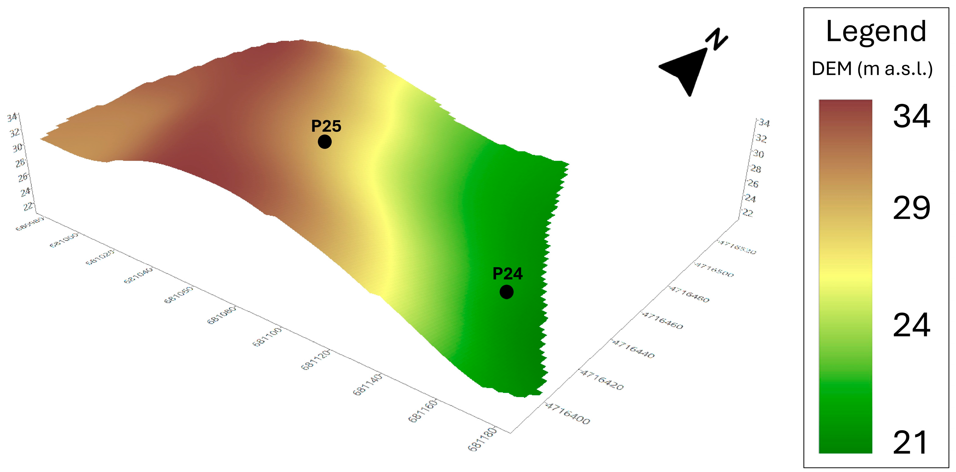
2.1. Study Area

The study field is a hazelnut orchard of approximately 2.5 hectares in size (Figure 1), situated in a hilly landscape of Grosseto province, Central Italy (42°34’45” N 11°12’22” E). This area is situated around 5 km from the coast of the Tyrrhenian Sea and is characterized by small hills with gentle slopes bordering the coastal plain. The area has recently been used for the cultivation of hazelnut trees, but the most common land uses are pastures, cereals, vineyards, and olive groves.

The climate is Mediterranean (Cs), according to Köppen’s classification, with an average precipitation of 550 mm, which is less frequent in the dry months, while it increases in the months following the summer season, and a mean annual temperature of 15.6 °C. According to the regional geological map, the study area is characterized by sandy and clayey marine deposits from the Early Pliocene [30]. The regional soil map reported the Eutric Cambisols as the most probable soils at this site, from loam to sandy clay loam in texture [31].

2.2. EMI Proximal Sensing

A proximal soil survey was carried out using the GF Mini Explorer EMI sensor by GF Instruments (Brno, Czech Republic). It consists of a system of a transmitting (Tx) coil, which operates at 30 kHz, and three receiving parallel coils (Rx), spaced 0.32, 0.71 and 1.18 m from the Tx. The survey was carried out with the coil in a vertical position, also called vertical coplanar mode (VCP). Such survey modality allows apparent electrical conductivity (ECa) to be detected at 3 different depths, typically 0–50 (ECa₁), 0–100 (ECa₂), and 0–150 cm (ECa₃). The sensor is also equipped with a GNSS system with a RTK correction to georeference the points detected and to obtain a map of the digital model of the terrain (DEM) with a resolution of 1 m, interpolating the measurement points by ordinary kriging. These information layers were used to perform a k-means clustering to individuate two homogeneous zones (HZ) in terms of morphology (DEM) and soil physical–hydrological features (ECa). The ECa and DEM data were normalized, from 0 (minimum value) to 1 (maximum value), before k-means clustering. Normalization and k-means clustering of the grids were carried out by SAGA-Gis 9.2.0 (System for Automated Geoscientific Analyses, www.saga-gis.org, accessed 4 December 2024). The soil of each HZ was described and analyzed by two soil profiles, dug near the extremes of ECa values, to a depth of about 1.2 m. The soils were classified according to WRB 2022 [32]. The polygons of HZs define the geometry of the soil map, whereas the description, analysis, and classification of the two soil profiles define the information of the soil typological units (STUs). This is the conventional and discrete soil mapping approach used by professional users and consultants working at field or farm scale. Although this discrete approach was commonly used in the soil mapping of small and medium fields, there is no information on the internal spatial variability of the STUs and no validation of the STU mapping.

2.3. NIR Spectroscopy

Producing accurate maps of soil spatial variability, also using geostatistics or spatial statistics analysis, implies collecting a minimum number of samples for laboratory analysis. To perform a kriging interpolation at the field scale, Ref. [33] proposed about 50 sampling units to perform a reliable semivariogram. In most cases, the collection and laboratory analysis of such a large number of samples, primarily for small and medium farms, is not cost-effective. To increase the number of datapoints with soil analysis without a relevant increase in costs for analysis, NIR spectroscopy was used. Covering the whole field area, 35 topsoil samples (0–30 cm) were randomly collected by augering for NIR spectroscopy.

The samples were dried at 30 °C and then passed through a sieve with a 2 mm mesh. Spectra were measured using Neospectra Scanner (NS), Si-Ware (USA), which is based on Micro-Electromechanical Systems (MEMS) Fourier transform (FT-NIR) technology. This type of sensor operates in the spectral range from 1350 to 2500 nm, with 252 bands at an original resolution of 16 nm, resampled by spline to 4.5 nm. Although the resolution was lower than that of traditional spectrometers, some recent studies demonstrated that the prediction accuracy of the most common soil features is comparable [27,28,29]. In addition, the source of the slightly higher prediction error of the FT-MEMS spectrometer was mainly due to the lack of the visible range rather than the instrument resolution [29].

NS was used on about 5 g of sieved soil placed in a laboratory glass dish and compressed only by the weight of the NS instrument. The NS was calibrated by its internal white reference about every 15 min.

A large spectral library characterized by spectra and associated laboratory analysis is needed to calibrate multivariate predictive models of soil features. The research group involved in this work is developing an Italian spectral library, performed by Neospectra Scanner, which includes 615 soil spectra. However, the spectral library was reduced to 362 spectra, removing forest soil samples, to include only soil samples from agricultural lands, different soil typologies, and different depths, although more than 70% belonged to the topsoil. To perform a site-specific calibration of NIR-based models, the spiking technique is one of the most used [33,34,35]. The principal aim of this method is to augment the calibration dataset with some samples of the target site, in order to achieve an improved estimation of a target soil variable. To increase the statistical weight of local samples within the general spectral library, some authors [33,35] proposed to add several copies of the spiking subset into the calibration matrix (extra-weight spiking). To select another three topsoil samples for laboratory analysis, representative of the variability of the entire data set, a k-means clustering based on the spectral data was used. The clustering used the 2 samples of the A horizons of the described profiles and the 35 topsoil samples collected by augerings. Five groups were selected for clustering. The two samples of the profiles, belonging to two different clusters (1 and 2), and one random member of each remaining cluster (3, 4 and 5) were selected for the calibration dataset and analyzed by traditional laboratory analysis. Laboratory analyses followed the official Italian protocol of soil analysis [36,37]. In particular, texture was analyzed by the pipette method, according to USDA textural thresholds; pH and EC were measured in a 1:5 soil-to-water solution; soil organic carbon (SOC) and total nitrogen by the humid methods of Walkley–Black and Kjeldhal, respectively; total carbonates by the gas–volumetric method using the Dietrich–Fruhling calcimeter; cation exchange capacity and exchangeable bases by extraction in a 1 N ammonium acetate solution.

The local calibration set (5) was then added in triplicate into the spectral library (SSL), following the extra-weighted spiking approach [36], reaching a total number of spectra of 377. The pre-treatments of the spectral library were as follows: (i) Savitzky–Golay filter through 5 points and a polynomial model to remove eventual noise; (ii) standard normal variate (SNV) to remove scattering effects (Figure 2).

Predictive models to determine sand, clay, soil organic carbon (SOC), total calcium carbonate (CaCO₃), cation exchange capacity (CEC), and total nitrogen (TN) were calibrated using partial least square regression (PLSR). PLSR is the most widely used multivariate statistical method in diffuse reflectance spectroscopy of soil samples and the most efficient method, as demonstrated in a recent review [26]. To determine the performance of PLSR in the prediction of local soil features, the PLSR validation was calculated only on the 5 local samples. The PLSR models of the soil features were used to predict the remaining datapoints (n = 32) not analyzed by traditional laboratory methods. Spectral pre-treatments, clustering, and PLSR were performed using Unscrambler X software 10.4 (Camo Software, Oslo, Norway).

2.4. Interpolation of the Maps and Validation

The soil features of the topsoil (0–30 cm), namely sand, clay, SOC, CaCO₃, CEC and TN, were interpolated within the study field, using (i) the data predicted by NIR and PLSR of the 32 augerings; (ii) the laboratory analysis of the A horizons of the two profiles (P24 and P25); and (iii) the laboratory analysis of the 3 augerings selected for calibration (T29, T36, T39). Therefore, the total datapoints for interpolation were 37 within a field of 2.5 hectares, but the datapoints analyzed with traditional laboratory methods were only 5, namely 2 analyses per hectare.

Such a limited number of datapoints (n = 37) did not allow the use of complex interpolation approaches like machine learning methods. Moreover, it can be assumed that the spatial distribution of the soil data was not stationary, since the field was characterized by two soil typologies (STUs) and slope morphology, and that probably the soil features were statistically correlated with environmental covariates. Therefore, the non-stationary interpolation method, namely kriging with external drift (KED), was used to spatialize the datapoints, using the digital elevation model (DEM), slope, the topographic wetness index (TWI), and the electrical conductivity of the shallowest layer (ECa₁), as covariates. Specifically, for each variable, only those covariates that showed significant correlation were selected and used, according to the values obtained through Pearson’s index. KED is a kriging technique with an external trend, calculated by a deterministic function between the target variable and the explanatory variables [38,39]. The interpolations were performed with Saga-Gis 9.2.0, using the universal kriging module. Universal kriging (UK) is often used as a synonym for KED, although several authors consider the two techniques to be different. The UK is a special case of kriging with a changing mean, where the trend is modelled as a function of coordinates [40]. If, instead of using the coordinates in the UK equations, the drift is defined externally through some auxiliary variables, the technique is called “kriging with external drift” [41]. The use of KED was preferred to other non-stationary methods based on regression, like regression kriging, because of moderate statistical relationships between target variables and covariates.

To measure the accuracy of the predicted maps, 5 additional augerings were carried out and analyzed. The locations of the validation augerings were randomly selected. From the differences between measured values and predicted values, extracted by the interpolated maps, the root mean square error (RMSE), bias, and coefficient of determination (R²) were calculated.

3. Results and Discussion

3.1. Maps Produced by EMI Proximal Survey

The proximal soil survey carried out by an electromagnetic induction (EMI) sensor showed the shallowest conductivity values (ECa₁ 0–50 cm), between 15 and 48 mS∙m⁻¹, with average values around the 20 mS∙m⁻¹ value; intermediate conductivity (ECa₂ 0–75 cm) showed values between 15 and 63 mS∙m⁻¹, whereas the deepest conductivity (ECa₃ 0–150 cm) varied between 15 and 61 mS∙m⁻¹. Higher conductivity values of ECa₂ and ECa₃ were mainly found in the central and southern part of the field and indicated a deep layer with high conductivity, probably characterized by high clay content. K-means clustering using the ECa layers (Figure 3) and the DEM (Figure 4) identified two potential soil typological units (STU). STU1 showed lower ECa values, on average 19 mS∙m⁻¹ for ECa₁ and 23 mS∙m⁻¹ for ECa₂ and ECa₃, but a mean higher altitude (30 m). STU2 showed higher ECa values, from 26 to 33 mS∙m⁻¹. Two profiles (Figure 4 and Figure 5) were dug to a depth of 1.5 m, to have a complete view and description of the soils. The analysis of the two profiles, reported in

Table 1. Descriptive statistics of the soil features of Profile P24.

Feature	Units	Ap 0–25 cm	Bw2 50–80 cm	Cg 90–110 cm
Clay	g·100 g−1	24	29	48
Sand	g·100 g−1	58	49	15
SOC	g·100 g−1	0.69	0.34	n.d.
TN	g·kg−1	0.77	0.43	n.d.
CEC	meq·100 g−1	18.3	21.95	n.d.
CaCO3	g·100 g−1	3.3	4.9	n.d.
pH		8.2	8.7	8.5
EC	mS·cm−1	0.26	0.38	0.50

and

Table 2. Descriptive statistics of the soil features of Profile P25. n.d.: not determined.

Feature	Units	Ap 0–25 cm	Bw2 50–75 cm	BC 90–110 cm
Clay	g·100 g−1	26	24	23
Sand	g·100 g−1	56	63	60
SOC	g·100 g−1	0.54	0.35	n.d.
TN	g·kg−1	0.62	0.43	n.d.
CEC	meq·100 g−1	17.94	18.11	n.d.
CaCO3	g·100 g−1	0.5	0.5	n.d.
pH		8.1	8.1	8.1
EC	mS·cm−1	0.14	0.15	0.15

, showed very similar features and analytical parameters in the shallower horizons A and Bw (0–75 cm). Both the soils showed a sandy clay loam texture and a low content of organic carbon (SOC) and calcium carbonate. The soil salinity, measured by laboratory electrical conductivity (EC, 1:5 solution), was always low (EC < 0.5 mS cm⁻¹), whereas the pH was sub-alkaline (8.2–8.4) and slightly alkaline (8.5–8.7) in the deeper horizons of P24 (Table 1).

The clearest difference between the soil profiles is due to the deepest horizon, deeper than 80 cm. P24 showed a Cg clayey horizon (clay = 48 g·100 g⁻¹), massive and characterized by a greyish color of strong redox conditions. On the contrary, P25 showed a BC horizon, scarcely structured, but with a texture similar to the topsoil (sandy clay loam). This clear difference between the deepest horizons was the main cause that discriminated the higher ECa values in STU 2, described by P24, compared to the lower ECa values of STU 1 (P25). Although the ECa₁ surveyed by Mini Explorer in VCP mode was indicatively referred to a depth of about 50 cm, the sensitivity of the electromagnetic field with respect to depth can be defined by functions, as reported by the instrument manual and by Bonsall et al. (2013) [42]. The function of Mini Explorer ECa₁ reported that about 80% of the sensitivity is between the surface and 0.5 m, but the remaining 20% of the sensitivity is calculated to a depth of about 2 m. Therefore, deep soil horizons partially affect the measurements of the shallowest ECa₁. For this reason, a theoretical field having homogeneous topsoil (0–50 cm) but different deep soil horizons can show spatial variability also in ECa₁. This is the case in this study field. The results obtained from the EMI sensor survey highlighted two very different areas: STU1, which is located at higher elevations, shows low and constant ECa values, probably related to a higher sand content, both in surface and in depth, as demonstrated by the analyses carried out on the P25 profile (Figure 6). STU2, which is in the lower part of the slope, showed a major increase in ECa between the surface layer (ECa₁) and the deeper layer (ECa₃), most likely due to the strong increase in clay with depth.

3.2. Topsoil Predicted by NIR

The analyzed samples collected by augerings (0–30 cm), three for calibration and five for validation, randomly taken within the field (Figure 7), showed moderate variability (

Table 3. Descriptive statistics of the soil features of 8 soil samples.

Feature	Units	Mean	SD	Min	Max
Clay	g·100 g−1	24	8.66	14	36
Sand	g·100 g−1	60	6.92	52	77
SOC	g·100 g−1	0.77	0.29	0.31	1.31
TN	g·kg−1	0.85	0.28	0.39	1.37
CEC	meq·100 g−1	18.89	3.98	13.08	24.32
CaCO3	g·100 g−1	2.38	2.71	0.5	8.3

). The sand content varied from 53 (T2) to 77 g·100 g⁻¹ (T33), clay from 14 (T33) to 36 g·100 g⁻¹ (T36); calcium carbonate (CaCO₃) was low (2–5 g·100 g⁻¹), although a few samples showed slightly higher values (T29 = 8. 3 g·100 g⁻¹). SOC showed mean values of 0.77 g·100 g⁻¹, whereas TN was 0.85 g·kg⁻¹, on average. The cation exchange capacity (CEC) had a mean of 18.9 cmol·kg⁻¹, with values ranging from 13.1 (T33) to 24.3 cmol·kg⁻¹ (T36). The NIR spectra of the three calibration augerings and of the soil horizons of the two profiles (P24 and P25) were included in the spectral library (in triplicate), as explained in the previous chapter, to perform PLSR predictive models. The total number of spectra used to carry out the PLSR predictive models was then 377, including 362 spectra of the SSL and five local samples (two profiles and three augerings) in triplicate.

Calibration of the PLSR models used nine factors for most of the variables, except for CEC and CaCO₃, which performed better with five and three factors, respectively. The PLSR predictions for clay, sand, and CEC show the lowest R² values, namely 0.76, 0.68, and 0.79, respectively. Higher R² values were calculated for SOC (0.93), TN (0.95), and CaCO₃ (0.95). The root mean square error of prediction (RMSEP), calculated only in the five local samples, as explained in the previous chapter, shows lower values for SOC (0.08 g·100 g⁻¹), TN (0.11 g·kg⁻¹), and CEC (1.27 cmol·kg⁻¹), but higher ones for CaCO₃ (2.19 g·100 g⁻¹), clay (4.98 g·100 g⁻¹) and sand (14.48 g·100 g⁻¹) (

Table 4. Results of PLSR models of NIR spectra to estimate clay, sand, SOC, TN, CEC and CaCO₃.

Variable		Loc 5
Clay	PLSR factors	9
	RMSEP (g·100 g−1)	4.98
	R2	0.76
Sand	PLSR factors	9
	RMSEP (g·100 g−1)	14.48
	R2	0.68
SOC	PLSR factors	9
	RMSEP (g·100 g−1)	0.08
	R2	0.93
TN	PLSR factors	9
	RMSEP (g·kg−1)	0.11
	R2	0.95
CEC	PLSR factors	5
	RMSEP (meq·100 g−1)	1.27
	R2	0.79
CaCO3	PLSR factors	3
	RMSEP (g·100 g−1)	2.19
	R2	0.95

). The results obtained by the PLSR models in terms of R² and RMSEP can be considered satisfactory for a quantitative prediction of the soil features. The prediction of sand was the only one with excessive RMSEP, although R² showed acceptable results. This was mainly due to a general underestimation of the model for this soil feature. A possible explanation could be given by the non-parametric distribution of the sand, both in the five local samples and in the total calibration set (global + local). Unfortunately, the distribution of the data,—homogeneous frequency for low and medium values, lower frequency for high values—did not allow us to apply efficient data transformations to improve the parametric distribution of the data. In the case of sand, we must accept a semi-quantitative prediction of the PLSR. In the context of laboratory analysis, cost is a critical variable, especially when a large number of samples are required for analysis. The introduction of near-infrared (NIR) spectroscopy has resulted in significant cost savings. In this work example, a lab-based methodology would have required 35 samples to be processed, whereas the use of NIR spectroscopy reduced this number to only five samples. Considering that the cost of soil analysis is between EUR 80 and EUR 100 per sample, the total cost of the analysis could be between EUR 2800 and EUR 3500. However, if only five samples were analyzed by a laboratory, and the rest of datapoints were predicted by NIR, the total costs for analysis could be reduced to around EUR 500, saving more than 80% of total costs. This technology makes it possible to obtain equally reliable information with far fewer samples, resulting in significant savings for companies facing routine or large-scale analysis.

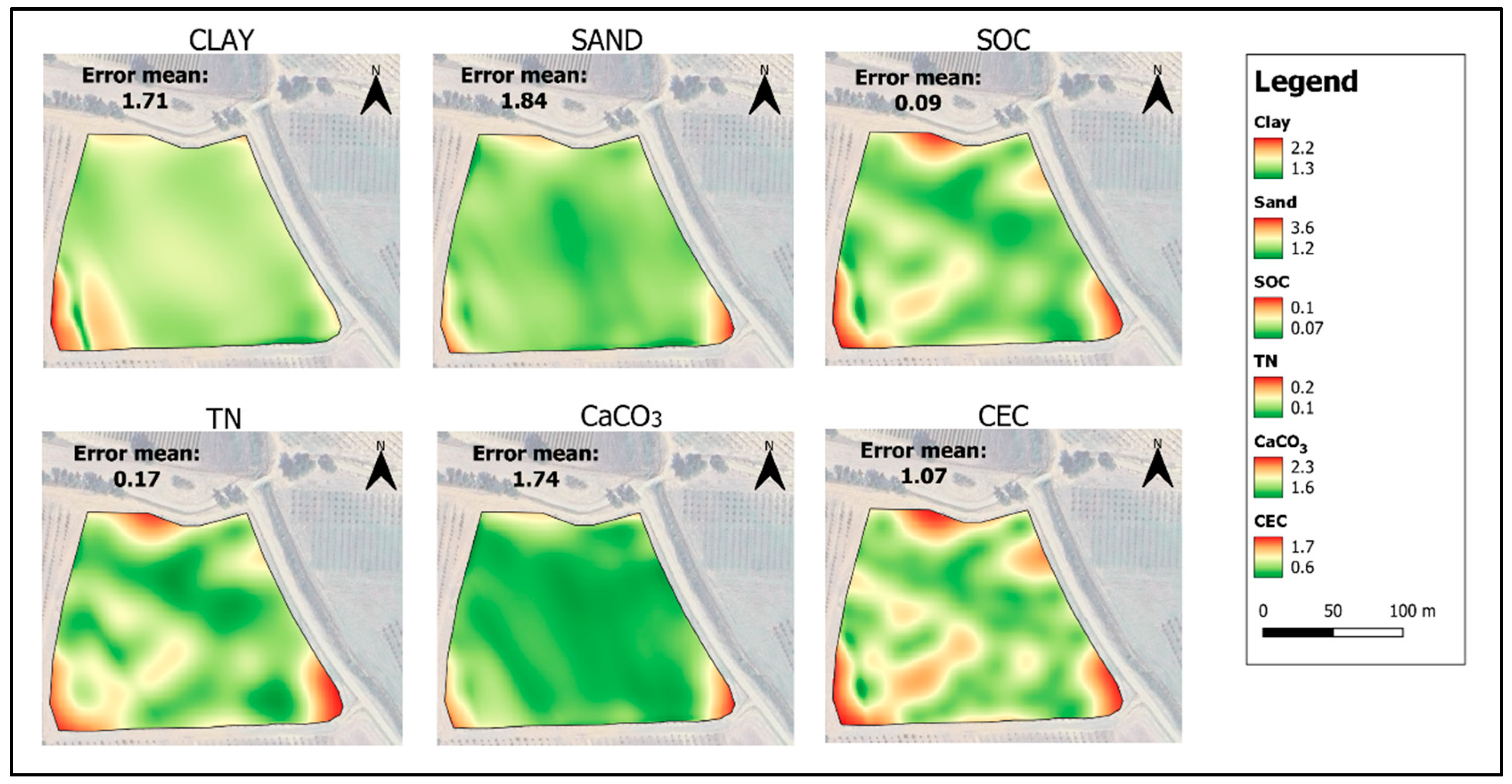
3.3. Interpolation of Topsoil Parameters

The maps of topsoil features were generated by the interpolation of the NIR predicted values (n = 32) and the five datapoints (two profiles and three augerings) analyzed by traditional laboratory analysis using kriging with external drift (KED). As already mentioned in the previous chapter, KED was preferred to other regression methods, such as regression kriging, because of the moderate statistical relationships between covariates and target variables (

Table 5. Pearson’s correlations between topsoil features, predicted by NIR, and covariates used for spatialization. In bold, significant correlations for p < 0.05.

	DEM	Slope	TWI	ECa1	ECa2	ECa3
Clay	0.561	0.111	−0.657	0.101	0.119	0.003
Sand	−0.304	−0.426	0.572	−0.161	−0.156	−0.055
SOC	−0.637	−0.241	0.678	−0.060	−0.042	0.131
TN	−0.244	−0.333	0.399	−0.207	−0.182	−0.074
CEC	0.642	−0.024	−0.563	−0.010	−0.001	−0.102
CaCO3	−0.129	0.440	−0.261	0.300	0.259	0.198

). The covariates selected as drift for KED were selected based on a significant correlation between the target variable and the covariates. Therefore, TWI was selected for all the interpolation models, whereas elevation (DEM) and slope were alternatively selected: the first for Clay, SOC and CEC; the second for sand, TN and CaCO₃ (Table 5).

Semivariogram modeling for kriging was possible with this number of datapoints (n = 37). The average distance between all pairs of sampling points was 85 m (median = 70 m), with a minimum distance of 9 m and a maximum distance of 190 m. To model the semivariograms of the different variables, a lag distance of 20–30 m and a range varying from 140 to 180 m were selected, according to the best semivariogram performance. Linear or Gaussian models were selected, according to the best performance (R²).

The maps obtained by KED show a variability from 20 to 32 g·100 g⁻¹ for clay, from 40 to 60 g·100 g⁻¹ for sand, and from 0.30 to 0.95 g·100 g⁻¹ for SOC (Figure 8), and a variability from 0.60 to 1.15 g·kg⁻¹ for TN, from 17 to 23 meq·100 g⁻¹ for CEC and from 0.02 and 8.80 g·100 g⁻¹ for CaCO₃ (Figure 9). The highest map errors occur for clay, sand and CaCO3 (Figure 10).

Table 6. Validation of the KED for clay, sand, SOC, TN, CEC, and CaCO₃. It was carried out on the 5 samples not used in the calibration model (T2, T11, T14, T23 and T33).

	R2	RMSE	BIAS
Clay	0.53	1.90	0.29
Sand	0.70	3.62	2.09
SOC	0.93	0.11	−0.07
TN	0.27	0.18	−0.14
CEC	0.46	1.62	0.46
CaCO3	0.49	2.84	−2.20

shows the results of the validation performed on the five additional samples (T2, T11, T14, T23, and T33), not used during PLSR or even during map interpolation (Figure 11). Although such a number of external validation points was very low, and then the calculation of errors could be highly subject to randomness, it is possible to verify the reliability of the soil feature spatialization in such a small field. Clay and sand predicted versus measured showed a good coefficient of determination (R² 0.53 and 0.70, respectively, Table 6), which demonstrates a good spatialization pattern. The RMSEP of these maps was low, at 1.90 and 3.62 g·100 g⁻¹, respectively. Better results were provided by the map of SOC, which showed R² of 0.93 and RMSEP of 0.11 g·100 g⁻¹, demonstrating a high accuracy of prediction. TN, CaCO₃, and CEC showed lower R² (0.27 to 0.49) but acceptable errors of prediction. These low R² together with the moderate error of prediction (RMSEP) can be explained by the low number of validation data used. For this reason, RMSEP data are more efficient for evaluating the reliability of the model with this low number of validation sampling points.

The method proposed in this work allows the discrete maps of soil typological units (STUs) of small fields to be improved, taking into account the spatial variability of the topsoil features, namely clay, sand, SOC, TN, CEC, and CaCO₃. The innovation of this approach is related to the very low number of samples required for traditional laboratory analysis, which includes the samples of the two soil profiles, describing the STUs, and three manual augerings, in a total surface area of about 2.5 hectares. The use of NIR spectroscopy allowed to increase the number of sampling points required for spatial interpolation of soil features, without significant costs.

4. Conclusions

The main objective of the study was to improve the accuracy of soil mapping of small- and medium-sized fields without significantly increasing the cost of analysis. The high cost of laboratory analysis did not allow a sampling frequency greater than 1–2 samples per hectare, which does not allow spatial interpolation of soil characteristics in small and medium fields. Although the grids correlated with soil features, such as DEM and ECa maps obtained by EMI proximal sensing, supported the interpolation of soil feature data, a minimum amount of data are required to perform spatial or regression analysis.

NIR spectroscopy and PLSR prediction allow the number of soil datapoints to be multiplied at low cost and appropriate spatial interpolation of the data to be performed. Kriging with external drift (KED), using the most correlated covariates as drift, produced accurate maps of clay, sand, and SOC, as well as fair accuracy for maps of TN, CEC, and CaCO₃.

Further improvements should be made in sampling strategies and in the use of other low-cost covariates, such as those derived from remote sensing, that can support and enhance spatial interpolation of soil characteristics.

References

1. Bramley, R.G. Lessons from nearly 20 years of Precision Agriculture research, development, and adoption as a guide to its appropriate application. Crop Pasture Sci. 2009, 60, 197–217. [Google Scholar] [CrossRef]
2. Viscarra Rossel, R.A.; Adamchuk, V.I. Proximal soil sensing. In Precision Agriculture for Sustainability and Environmental Protection; Earthscan: Oxford, UK, 2013; pp. 99–118. [Google Scholar] [CrossRef]
3. Hedley, C.B.; Yule, I.J.; Eastwood, C.R.; Shepherd, T.G.; Arnold, G. Rapid identification of soil textural and management zones using electromagnetic induction sensing of soils. Soil Res. 2004, 42, 389–400. [Google Scholar] [CrossRef]
4. Castrignanò, A.; Buttafuoco, G.; Quarto, R.; Vitti, C.; Langella, G.; Terribile, F.; Venezia, A. A combined approach of sensor data fusion and multivariate geostatistics for delineation of homogeneous zones in an agricultural field. Sensors 2017, 17, 2794. [Google Scholar] [CrossRef] [PubMed]
5. Adhikari, K.; Smith, D.R.; Collins, H.; Hajda, C.; Acharya, B.S.; Owens, P.R. Mapping within-field soil health variations using apparent electrical conductivity, topography, and machine learning. Agronomy 2022, 12, 1019. [Google Scholar] [CrossRef]
6. Ji, W.; Adamchuk, V.I.; Chen, S.; Su, A.S.M.; Ismail, A.; Gan, Q.; Shi, Z.; Biswas, A. Simultaneous measurement of multiple soil properties through proximal sensor data fusion: A case study. Geoderma 2019, 341, 111–128. [Google Scholar] [CrossRef]
7. Vasques, G.M.; Rodrigues, H.M.; Coelho, M.R.; Baca, J.F.M.; Dart, R.O.; Oliveira, R.P.; Teixeira, W.G.; Ceddia, M.B. Field Proximal Soil Sensor Fusion for Improving High-Resolution Soil Property Maps. Soil Syst. 2020, 4, 52. [Google Scholar] [CrossRef]
8. Andrade, R.; Silva, S.H.G.; Faria, W.M.; Poggere, G.C.; Barbosa, J.Z.; Guilherme, L.R.G.; Curi, N. Proximal sensing applied to soil texture prediction and mapping in Brazil. Geoderma Reg. 2020, 23, e00321. [Google Scholar] [CrossRef]
9. Priori, S.; Barbetti, R.; Meini, L.; Morelli, A.; Zampolli, A.; D’avino, L. Towards economic land evaluation at the farm scale based on soil physical-hydrological features and ecosystem services. Water 2019, 11, 1527. [Google Scholar] [CrossRef]
10. Becker, S.M.; Franz, T.E.; Abimbola, O.; Steele, D.D.; Flores, J.P.; Jia, X.; Scherer, T.F.; Rudnick, D.R.; Neale, C.M. Feasibility assessment on use of proximal geophysical sensors to support precision management. Vadose Zone J. 2022, 21, e20228. [Google Scholar] [CrossRef]
11. Martelli, R.; Civitarese, V.; Barbanti, L.; Ali, A.; Sperandio, G.; Acampora, A.; Misturini, D.; Assirelli, A. Multi-Parametric Approach to Management Zone Delineation in a Hazelnut Grove in Italy. Sustainability 2023, 15, 10106. [Google Scholar] [CrossRef]
12. Doolittle, J.A.; Brevik, E.C. The use of electromagnetic induction techniques in soils studies. Geoderma 2014, 223, 33–45. [Google Scholar] [CrossRef]
13. Rhoades, J.D.; Manteghi, N.A.; Shouse, P.J.; Alves, W.J. Soil electrical conductivity and soil salinity: New formulations and calibrations. Soil Sci. Soc. Am. J. 1989, 53, 433–439. [Google Scholar] [CrossRef]
14. Corwin, D.L.; Lesch, S.M. Apparent soil electrical conductivity measurements in agriculture. Comput. Electron. Agric. 2005, 46, 11–43. [Google Scholar] [CrossRef]
15. Sudduth, K.A.; Drummond, S.T.; Kitchen, N.R. Accuracy issues in electromagnetic induction sensing of soil electrical conductivity for precision agriculture. Comput. Electron. Agric. 2001, 31, 239–264. [Google Scholar] [CrossRef]
16. Corwin, D.L.; Scudiero, E. Field-scale apparent soil electrical conductivity. Soil Sci. Soc. Am. J. 2020, 84, 1405–1441. [Google Scholar] [CrossRef]
17. Martini, E.; Werban, U.; Zacharias, S.; Pohle, M.; Dietrich, P.; Wollschläger, U. Repeated electromagnetic induction measurements for mapping soil moisture at the field scale: Validation with data from a wireless soil moisture monitoring network. Hydrol. Earth Syst. Sci. 2017, 21, 495–513. [Google Scholar] [CrossRef]
18. Piikki, K.; Wetterlind, J.; Söderström, M.; Stenberg, B. Three-dimensional digital soil mapping of agricultural fields by integration of multiple proximal sensor data obtained from different sensing methods. Precis. Agric. 2015, 16, 29–45. [Google Scholar] [CrossRef]
19. Ciampalini, A.; André, F.; Garfagnoli, F.; Grandjean, G.; Lambot, S.; Chiarantini, L.; Moretti, S. Improved estimation of soil clay content by the fusion of remote hyperspectral and proximal geophysical sensing. J. Appl. Geophys. 2015, 116, 135–145. [Google Scholar] [CrossRef]
20. Rossel, R.V.; McBratney, A.B. Soil chemical analytical accuracy and costs: Implications from precision agriculture. Aust. J. Exp. Agric. 1998, 38, 765–775. [Google Scholar] [CrossRef]
21. Wetterlind, J.; Stenberg, B.; Söderström, M. The use of near infrared (NIR) spectroscopy to improve soil mapping at the farm scale. Precis. Agric. 2008, 9, 57–69. [Google Scholar] [CrossRef]
22. Conforti, M.; Matteucci, G.; Buttafuoco, G. Using laboratory Vis-NIR spectroscopy for monitoring some forest soil properties. J. Soils Sediments 2018, 18, 1009–1019. [Google Scholar] [CrossRef]
23. Jaconi, A.; Vos, C.; Don, A. Near infrared spectroscopy as an easy and precise method to estimate soil texture. Geoderma 2019, 337, 906–913. [Google Scholar] [CrossRef]
24. Leone, A.P.; Leone, G.; Leone, N.; Galeone, C.; Grilli, E.; Orefice, N.; Ancona, V. Capability of Diffuse Reflectance Spectroscopy to Predict Soil Water Retention and Related Soil Properties in an Irrigated Lowland District of Southern Italy. Water 2019, 11, 1712. [Google Scholar] [CrossRef]
25. Zhao, D.; Arshad, M.; Li, N.; Triantafilis, J. Predicting soil physical and chemical properties using vis-NIR in Australian cotton areas. Catena 2021, 196, 104938. [Google Scholar] [CrossRef]
26. Ahmadi, A.; Emami, M.; Daccache, A.; He, L. Soil properties prediction for precision agriculture using visible and near-infrared spectroscopy: A systematic review and meta-analysis. Agronomy 2021, 11, 433. [Google Scholar] [CrossRef]
27. Ng, W.; Anggria, L.; Siregar, A.F.; Hartatik, W.; Sulaeman, Y.; Jones, E.; Minasny, B. Developing a soil spectral library using a low-cost NIR spectrometer for precision fertilization in Indonesia. Geoderma Reg. 2020, 22, e00319. [Google Scholar] [CrossRef]
28. Thomas, F.; Petzold, R.; Becker, C.; Werban, U. Application of Low-Cost MEMS Spectrometers for Forest Topsoil Properties Prediction. Sensors 2021, 21, 3927. [Google Scholar] [CrossRef]
29. Priori, S.; Mzid, N.; Pascucci, S.; Pignatti, S.; Casa, R. Performance of a Portable FT-NIR MEMS Spectrometer to Predict Soil Features. Soil Syst. 2022, 6, 66. [Google Scholar] [CrossRef]
30. Available online: https://www502.regione.toscana.it/geoscopio/geologia.html (accessed on 4 December 2024).
31. IUSS Working Group WRB. World reference base for soil resources. In International Soil Classification System for Naming Soils and Creating Legends for Soil Maps, 4th ed.; International Union of Soil Sciences (IUSS): Vienna, Austria, 2022. [Google Scholar]
32. Kerry, R.; Oliver, M.A. Comparing sampling needs for variograms of soil properties computed by the method of moments and residual maximum likelihood. Geoderma 2007, 140, 383–396. [Google Scholar] [CrossRef]
33. Guerrero, C.; Stenberg, B.; Wetterlind, J.; Viscarra Rossel, R.A.; Maestre, F.T.; Mouazen, A.M.; Zornoza, R.; Ruiz-Sinoga, J.D.; Kuang, B. Assessment of soil organic carbon at local scale with spiked NIR calibrations: Effects of selection and extra-weighting on the spiking subset. Eur. J. Soil Sci. 2014, 65, 248–263. [Google Scholar] [CrossRef]
34. Nawar, S.; Mouazen, A.M. Predictive performance of mobile vis-near infrared spectroscopy for key soil properties at different geographical scales by using spiking and data mining techniques. Catena 2017, 151, 118–129. [Google Scholar] [CrossRef]
35. Seidel, M.; Hutengs, C.; Ludwig, B.; Thiele-Bruhn, S.; Vohland, M. Strategies for the efficient estimation of soil organic carbon at the field scale with vis-NIR spectroscopy: Spectral libraries and spiking vs. local calibrations. Geoderma 2019, 354, 113856. [Google Scholar] [CrossRef]
36. MIPAF-Ministero per le Politiche Agricole e Forestali. Metodi Ufficiali di Analisi Fisica del Suolo. DM 1st August 1997, Gazzetta Ufficiale n. 204, 2/09/97. 1997. Available online: https://www.gazzettaufficiale.it/eli/id/1997/09/02/097A6592/sg (accessed on 4 December 2024).
37. MIPAF-Ministero per le Politiche Agricole e Forestali. Metodi Ufficiali di Analisi Chimica del Suolo. DM 13/09/99, Gazzetta Ufficiale n. 204, 21/10/99. 1999. Available online: https://www.gazzettaufficiale.it/eli/id/1999/10/21/099A8497/sg (accessed on 4 December 2024).
38. Nielsen, D.R.; Wendroth, O. Spatial and Temporal Statistics. Geoecology Textbook; Catena Verlag GMBH: Reiskirchen, Germany, 2003. [Google Scholar] [CrossRef]
39. Webster, R.; Oliver, M.A. Geostatistics for Environmental Scientists; John Wiley & Sons: Hoboken, NJ, USA, 2007. [Google Scholar] [CrossRef]
40. Matheron, G. Le krigeage Universel. Vol. 1. Cahiers du Centre de Morphologie Mathematique; Ecole des Mines de Paris: Fontainebleau, Paris, France, 1969. [Google Scholar] [CrossRef]
41. Hengl, T.; Geuvelink, G.B.M.; Stein, A. Comparison of Kriging with External Drift and Regression-Kriging; Technical Note; ITC: Tokyo, Japan, 2003. [Google Scholar]
42. Bonsall, J.; Fry, R.; Gaffney, C.; Armit, I.; Beck, A.; Gaffney, V. Assessment of the CMD mini-explorer, a new low-frequency multi-coil electromagnetic device, for archaeological investigations. Archaeol. Prospect. 2013, 20, 219–231. [Google Scholar] [CrossRef]
Figure 1. Framework for the study area.
Soilsystems 08 00128 g001
Figure 2. Pretreatments applied to the spectral library with local samples (n = 377): on the left the Savitzky–Golay filter; on the right, the application of the standard normal variate.
Soilsystems 08 00128 g002
Figure 3. Maps of electrical conductivity (ECa) measured at different depths by EMI sensor. The black dots show the soil profiles (P24 and P25), whereas the polygons show the two STUs delineated by k-means clustering.
Soilsystems 08 00128 g003
Figure 4. Digital elevation model (DEM) with selected profiles.
Soilsystems 08 00128 g004
Figure 5. Profile P24.
Soilsystems 08 00128 g005
Figure 6. Profile P25.
Soilsystems 08 00128 g006
Figure 7. Total random augerings. The blue dots are the points selected for the local calibration set.
Soilsystems 08 00128 g007
Figure 8. Maps of clay (g·100 g−1), sand (g·100 g−1) and SOC (g·100 g−1), interpolated by KED, using the values of the sampling datapoints predicted by NIR spectroscopy and the most related covariates according to Pearson’s correlation index.
Soilsystems 08 00128 g008
Figure 9. Maps of TN (g·kg−1), CEC (meq·100 g−1) and CaCO3 (g·100 g−1), interpolated by KED, using the values of the sampling datapoints predicted by NIR spectroscopy and the most related covariates according to Pearson’s correlation index.
Soilsystems 08 00128 g009
Figure 10. Error map of clay (g·100 g−1), sand (g·100 g−1), SOC (g·100 g−1), TN (g·kg−1), CEC (meq·100 g−1), and CaCO3 (g·100 g−1), interpolated by KED, using the values of the sampling datapoints predicted by NIR spectroscopy and the most related covariates according to Pearson’s index.
Soilsystems 08 00128 g010
Figure 11. Total random augerings. Blue dots are the points selected for the local calibration set; red dots are the points collected for the local validation set.
Soilsystems 08 00128 g011