Article

Environmental Impact of Sulaimani Steel Plant (Kurdistan Region, Iraq) on Soil Geochemistry

by
Roshna A. Hamarashid
1,*,
Željka Fiket
2 and
Ibrahim M. J. Mohialdeen
1
1
Department of Geology, College of Science, University of Sulaimani, Sulaymaniyah 334, Iraq
2
Divison for Marine and Environmental Research, Ruđer Bošković Institute, 10000 Zagreb, Croatia
*
Author to whom correspondence should be addressed.
Soil Syst. 2022, 6(4), 86; https://doi.org/10.3390/soilsystems6040086
Submission received: 13 September 2022 / Revised: 8 November 2022 / Accepted: 15 November 2022 / Published: 18 November 2022

Abstract

:
Steel is an indispensable material that is used in a wide range of products and that contributes significantly to economic development. However, steel production can affect soil quality and is associated with the pollution of local areas. Therefore, the objective of this study was to investigate the mineral and geochemical composition of soils in the vicinity of the Sulaimani Steel Plant (SSP) in Bazian Region, Kurdistan, Iraq. A total of 35 soil samples were collected in the vicinity of SSP. The samples were analyzed for their mineral and geochemical composition, including 10 major, and 40 trace and rare earth elements. In addition, the soils were analyzed for their particle size distribution, pH, and organic matter content. The distribution of elements in the soils was found to be influenced by the texture, organic matter content (0.34–9.28%), and prevailing wind direction. The assessment of soil contamination near the steel plant confirmed high to extremely high enrichment with Cr (EF up to 20.7), Ni (EF up to 14.2), Pb (EF up to 80.4), and Th (EF up to 50.4), indicating that it is a significant source of heavy metals and poses a high risk to soil health.

1. Introduction

The future of environmental management is based on predictive models for assessing the impacts and pollution risks resulting from the indiscriminate use of natural resources and harmful anthropogenic substances [1] and their application in various production plants, including steel mills. In the last 20 years, environmental issues have become a widespread national concern, although “environment” has not always been an issue [2]. In this sense, steel mills also contribute negatively, considering that the demand for steel has increased to 1.4 billion tons per year and is expected to double by 2050, with the steel industry responsible for about one-tenth of global energy-related CO2 emissions [3]. Indeed, steel production is responsible for a quarter of all industrial CO2 emissions and 9% of global CO2 emissions from energy and industrial processes. This makes the steel industry’s carbon footprint the largest of all industrial sectors [4]. In addition, iron and steel production generates waste products such as slag, which is enriched with many heavy metals (e.g., Mn, Zn, and Pb [5]). Some volatile trace metals are released into the environment by atmospheric processes and particulate emissions [6]. Such airborne particles settle in the environment after leaving the plant and affect the soil quality in the area, which is often used by local residents as a recreational area or for agricultural purposes. As a result, soil pollution is increasingly becoming a problem for the environment and human health [7]. Despite the fact that soil acts as a filter for purifying and immobilizing many pollutants [8], and despite regulations and chemical standards enacted to maintain soil health [9], sites near steel and iron works continue to be heavily polluted by operational activities. Schulin et al. [10] studied the heavy metal contamination of the soil near a Bulgarian ironworks. It was found that the dust emitted from the ironworks polluted the agricultural soils near the ironworks with As, Pb and Zn. Yuan et al. [11] conducted a comprehensive study to evaluate the quality of topsoil near an abandoned steel smelter in Beijing, China, and found greater amounts of Cu, Pb, Cd, and Zn compared to background levels. Mohiuddin et al. [12] studied the distribution of trace metals in atmospheric particles near the iron and steel industry sites in Australia. The authors found significantly higher concentrations of trace metals such as Co, Cr, Cu, Fe, Mn, Ni, Ti, V, and Zn in the atmospheric particles collected in areas near iron and steel industry sites compared to background levels, and they were differently related to the size fractions. Akporido et al. [13] showed the impact of steel production on soil quality in the Udu section of the Warri River near a steel plant in Nigeria. They found that the sampling sites near the steel plant were more polluted with heavy metals Fe, Pb, Cd, Ni and Zn than the other sites. Namuhani and Kimumwe [14] evaluated the heavy metal contamination of soil near steel rolling mills in Jinja municipality, Uganda. The concentrations of the heavy metals Cu and Cd near the rolling mill showed moderate and moderate to severe pollution, respectively. Ladonin [15] studied the rare earth elements (REEs) in soils at different distances from the Cherepovets steel plant in Vologda oblast, Russia, and found that the levels of Pr and Tb were higher in soils near the plant. Previous studies in the Bazian region mainly investigated the chemical and biological properties of air, groundwater, and soil as well as oil reservoirs [16,17,18,19]. Mohialdeen et al. [16] studied the geochemistry of crude oil from a near-surface well in the Bazian region. They concluded that the origin of the heavy oil was in the Kolosh formation. Rasheed and Faqesaleh [17] studied the evaluation of some heavy metals in the water and soil of a Bazian oil refinery. They found that the plant has a significant impact on the pollution of groundwater and soil by the heavy metals Cr, Pb, Cd, Cu, Zn, and Ni. Al-Taay et al. [18] studied the impact of a Bazian cement plant on water and found that the concentrations of various heavy metals such as Cd, Cr, Pb, Cu, Ni, Fe and Zn were similar to background levels. Ahmed [19] described the mapping of groundwater potential and well protection areas in Bazian sub-basin. Hamakarim [20] studied the assessment of some heavy metals in soils surrounding scrap metal recycling factories in the Sulaimani governorate, Iraq. The authors found that the spatial distribution of the studied metals decreased in the following order: Fe > Mn > Ni > Cr > V > Co, while the pollution indices only indicate minor pollution. However, no studies have examined the effects of the Sulaimani Steel Plant on the composition of the surrounding soils, although such and similar plants are known to be sources of numerous heavy metals [10,11,12,13], which can have various adverse effects on the soil and environmental health.
Therefore, the aim of this study was to determine the geochemical composition of the soil in the vicinity of the Sulaimani steel plant (SSP) and to investigate the impact of the steel plant on the surrounding soils by, also taking into account the prevailing wind directions as the predominant direction of material transport. For this purpose, the concentrations of selected major and trace elements, including rare earth elements, as well as the organic matter content and grain size distribution were studied in soil samples collected near the Sulaimani steel plant.

2. Materials and Methods

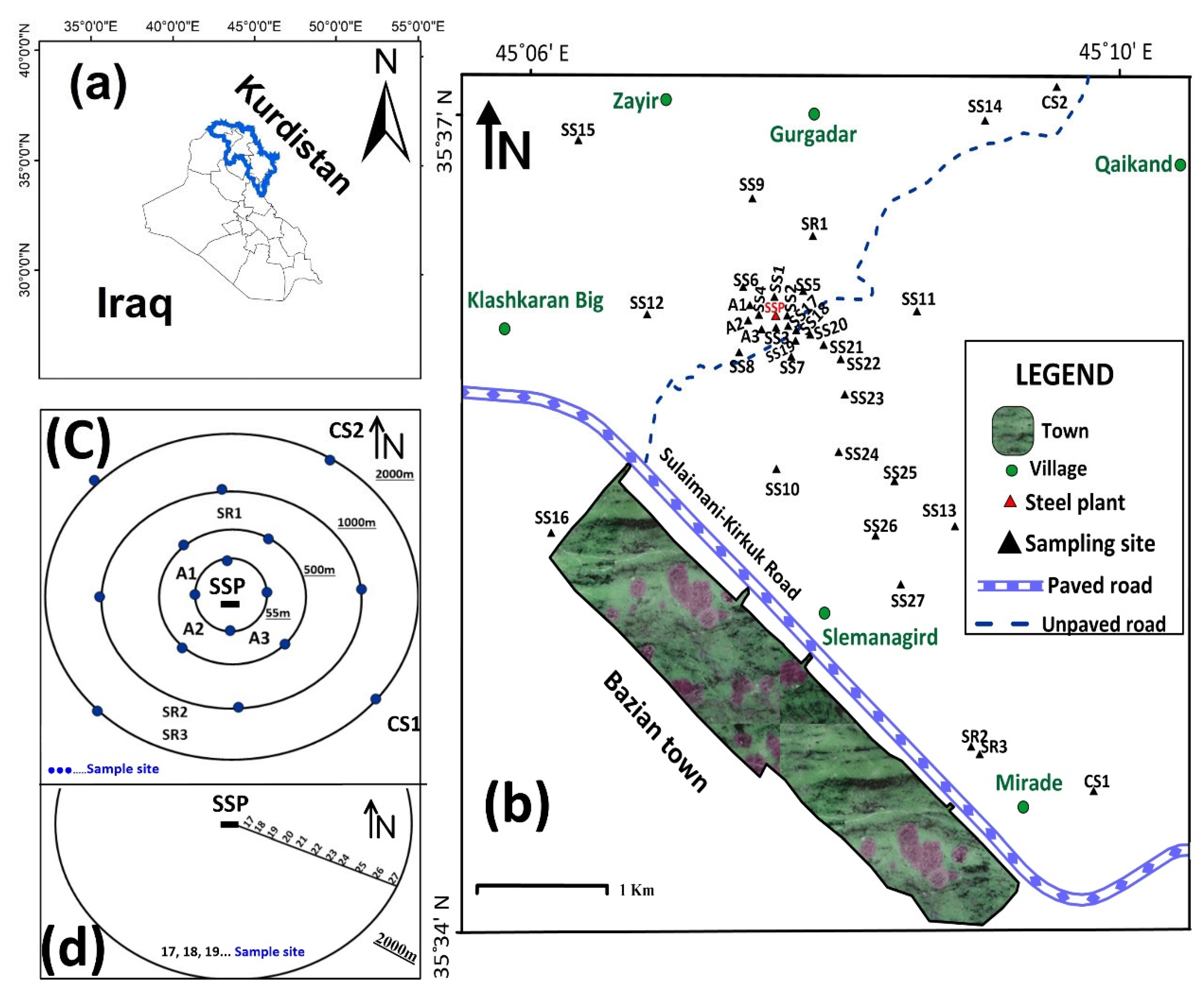
2.1. Geologic Setting and the Study Area

The SSP site is located on the main Sulaimani-Kirkuk road in the town of Bazian, approximately 30 km west of the city of Sulaimani in the Kurdistan Region of Iraq (Figure 1a,b). Tectonically, the Bazian Basin is located within a High Fold Zone (HFZ), and the area has been strongly deformed due to strong tectonic activity at an earlier geologic time [21]. According to Hamamin [22], the main lithostratigraphic units from the oldest to the youngest in this area are the following formations: the Kolosh Formation, Sinjar Formation, Gercus Formation, Pila-Spi Formation and finally Quaternary deposits. SSP was built on Tasluja Mountains, which are mainly the Sinjar Formation, and SSP, is mainly located on the Sinjar Formation and partly on theKolosh Formation. The Kolosh Formation is deposited as flysch facies of sandstones, marls, shales, intraformative conglomerates and thin beds of arenic limestone. Recently, Ahmad [23] stated that the Sinjar Formation consists of a thick, massive and extremely fossiliferous limestone with occasional layers of dolomitic limestone.

2.2. Sampling and Sample Preparation

The sampling campaign was conducted in August and September 2021 in the vicinity of the Sulaimani steel plant in Kurdistan region, Iraq (Figure 1a,b). A total of 35 samples, including 32 soil samples and three source rock samples, were collected at varying distances from SSP (Figure 1c,d). Three soil samples were collected near the plant (A1, A2 and A3) and 16 soil samples were collected at 55 m, 500 m, 1000 m and 2000 m from SSP (Figure 1c). Three samples of local source rock (SR1, SR2, and SR3) and two reference soil samples (CS1 and CS2) were also collected. According to wind direction and prevailing air currents, the greatest environmental impact of SSP was expected to be in the east and southeast directions. Therefore, an additional 11 samples were collected at different distances from SSP: 55 m, 100 m, 150 m, 200 m, 300 m, 500 m, 750 m, 1000 m, 1250 m, 1500 m, and 2000 m (Figure 1d). In general, the soils are reddish-brown in color and only contain a sporadic gravel fraction. The GPS coordinates of the sampling sites are listed in Table S1.
At each site, approximately 1 kg of topsoil (the first 10 cm) was collected with a shovel and stored in plastic containers. In the laboratory, the soil samples were air dried, homogenized, and sieved through a 2 mm sieve to remove pebbles and biota. The samples prepared in this way were subjected to granulometric analysis, while the remaining samples were pulverized and stored for other analyses.
Prior to trace element analysis, soil sub-samples (0.05 g) were subjected to total digestion in a microwave oven (Multiwave 3000, Anton Paar, Graz, Austria). The procedure consisted of digestion with a mixture of 4 mL nitric acid (HNO3, 65%, pro analysi, Kemika, Zagreb, Croatia), 1 mL hydrochloric acid (HCl) and 1 mL hydrofluoric acid (HF, 48%, pro analysi, Kemika, Zagreb, Croatia), followed by the addition of 6 mL boric acid (H3BO3, Fluka, Steinheim, Switzerland). Prior to analysis, the digests were diluted tenfold, acidified with 2% (v/v) HNO3 (65%, supra pure, Fluka, Steinheim, Switzerland), and In (1 μg L−1) was added as an internal standard. A detailed method description is given elsewhere [24].

2.3. Sample Analysis

2.3.1. Grain Size Distribution

Grain size distribution analysis was performed on all sediment samples except SR1. The analysis was conducted at the Sulaimani construction laboratory according to ASTM standards using sieve and hydrometer analysis [25] and specific gravity [26].

2.3.2. Organic Matter Content and pH

Total organic carbon (TOC) was determined for all described samples using the method described by El-Wakeel and Riley [27], while the organic matter content (OM) was calculated as follows [28]:
% Organic Matter = % Total Organic Carbon × 1.724
The pH was determined with a multimeter in a suspension with a 1:10 ratio of soil and liquid phase according to the following protocol: 5 g of the soil sample was mixed with 50 mL of deionized water and measured with a pH meter (Hanna Instruments, Woonsocket, RI, USA).

2.3.3. Mineral Composition

Mineral composition analysis was performed by X-ray powder diffraction (XRPD, Bruker D8 Advanced, Bruker AXS GmbH, Karlsruhe, Germany) at XRD Laboratory, East Amethyst, Pardis Science and Technology Park, Iran, for all of the samples studied. X-ray diffraction was performed using anX’Pert analytical powder diffractometer with Cu-Kα radiation (λ = 1.542 Å) at a voltage of 40 kV and a beam current of 30 mA with 10 counts/s over a 2θ range from 4° to 60° and a step size of 0.02°.

2.3.4. XRF Measurements

The content of the major elements in soil was determined by X-ray fluorescence (Panalytical XRF, PANalytical B.V., Almelo, The Netherlands) at the XRF Laboratory, East Amethyst, Pardis Science and Technology Park, Iran, and reported as oxides. Analytical uncertainties ranged from 0.04% to 0.1% for the major elements. The detection limit for the major oxides was 0.002–0.04 wt%. The total loss on ignition (LOI) was estimated from the weight difference after annealing at 1000 °C using Master Data Management (M D M) and was −5.1%.

2.3.5. ICP-MS Measurements

Multielement analysis of the prepared soil digests was performed by high-resolution inductively coupled plasma mass spectrometry (HR ICP-MS) using an Element 2 instrument (Thermo, Bremen, Germany) at the Ruđer Bošković Institute in Zagreb, Croatia. The typical instrument conditions and measurement parameters used throughout the work are presented in Table 1.
All samples were analyzed for the total concentration of 40 elements (As, Ba, Be, Bi, Cd, Ce, Co, Cr, Cs, Cu, Dy, Er, Eu, Gd, Ho, La, Li, Lu, Mo, Nd, Ni, P, Pb, Pr, Rb, S, Sb, Sc, Sm, Sn, Sr, Tb, Tl, Tm, U, V, Y, Yb, and Zn). Quality control of the analytical procedure was performed by simultaneous analysis of the blank sample and the certified reference material for soil (NCS DC 77.302, China National Analysis Center for Iron and Steel, Beijing, China). Good agreement was obtained for all elements between the analyzed and certified concentrations within their analytical uncertainties (~10%).

2.4. Data Analysis

2.4.1. Statistical Analysis

In this study, matrix and correlation coefficient analyses were applied to the geochemical data using STATISTICA and SPSS 26 programs, and principal component analysis (PCA) was used to determine the relationships among elements around SSP. Alpine Quest with Grapher software were used to generate maps, while Surfer (version 16, Golden Software, Golden, CO, USA) was used to determine the pollution intensity of heavy metals and REE. Grapher (version 16, Golden Software, Golden, CO, USA) was used for normalization plots and for the spatial distribution of the REE concentration in the study area.

2.4.2. The Assessment of Soil Pollution

Different calculation approaches have been used to evaluate the degree of metal enrichment in sediments and soils [29,30,31]. In this study, the enrichment factors [32] and the geoaccumulation index [33] were used to evaluate the degree of contamination and metal distribution in the vicinity of SSP.
The enrichment factor (EF) is a common normalization method for classifying metal enrichment in soils or sediments. To identify anomalous metal contents, geochemical normalization of metal data is applied to conservative elements such as Al, Fe, or Si. Al was used in the present study. The EF is defined as follows:
EF = ( C x / C A l   ) s a m p l e ( B x / B A l   ) b a c k g r o u n d
where Cx and CAl (sample) are the concentrations of an investigated element x and a reference element, respectively, in a soil sample, while Bx and BAl (background) are the concentrations of an investigated element x and a reference element, respectively, in the background
According to Loska et al. [32], there are the following contamination categories: insufficient to minimal enrichment (EF < 2), moderate enrichment (EF = 2–5), significant enrichment (EF = 5–20), very high enrichment (EF = 20–40), and extremely high enrichment (EF > 40).
The geoaccumulation index (Igeo) proposed by Ref. [33] is calculated to estimate the degree of soil contamination using seven accumulation classes based on the increasing numerical values of the index. This index is calculated as follows:
I g e o = log 2 C x 1.5 B x
where Cx is the content of element x in the soil sample and Bx is the background value of element x according to Kabata-Pendias and Mukherjee [34] for trace elements and Rudnick and Gao [35] for REEs. The factor of 1.5 is introduced to minimize the effects of possible variations in background values that may be due to lithological variations in the sediment. As described in Ref. [33], there are six Igeo classes: practically uncontaminated (Igeo ≤ 0), uncontaminated to moderately contaminated (0 < Igeo < 1), moderately contaminated (1 < Igeo < 2), moderately to heavily contaminated (2 < Igeo < 3), heavily contaminated (3 < Igeo < 4), heavily to extremely contaminated (4 < Igeo < 5), and extremely contaminated (5 < Igeo).

3. Results

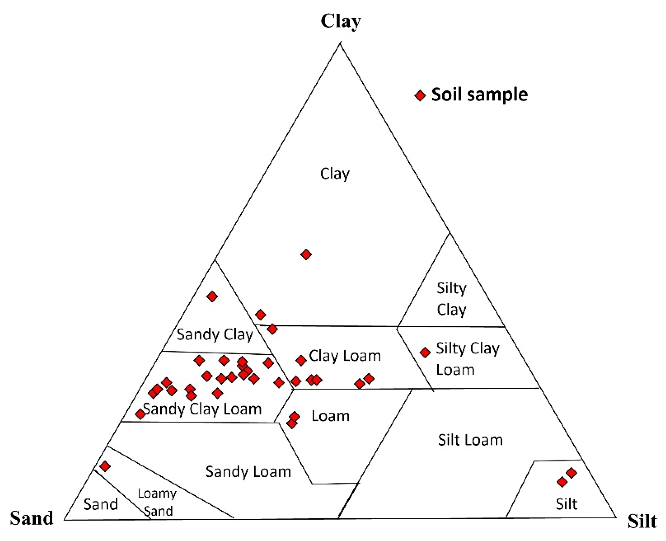
3.1. Grain Size Analysis

Based on the results of the grain size analysis of the surface sediments in the study area, clay is the predominant grain size (average 51%), followed by silt and sand with 27% and 22%, respectively (Table 2). According to the USDA ternary diagram [36], the sediment samples are classified as sandy loam to clay loam (Figure 2). The clay content varies from 3.18% to 87.3%. At most sites, the clay content exceeds 70%, such as at sites SS10, SS14, SS23, and CS1 with 73.4%, 74.6%, 76.8%, and 87.2%, respectively. The silt content in these samples ranged from 6.02% to 57.1%, while the sand content was very heterogeneous (2.6–88.9%). The highest silt content was found in the soils at sites CS2, SS24 and SS9 with 57.1%, 42.7% and 41.4%, respectively (Table 2).

3.2. Organic Matter (OM) Content and pH Value

As shown in Table 2, the content of organic matter in the samples studied ranged from 1.48 to 9.28%. The lowest value of OM (1.48%) was found at site SS18, while the highest value (9.28%) was found at site SS22. The pH values of the studied soils varied from 8.22 to 9.92 (Table 2). The lowest pH value (8.22) was obtained at site SS13, but the highest pH value (9.92) was obtained at site SR1.

3.3. Mineralogy of Studied Soils

In Table 3, the bulk and clay mineralogy of studied soils is presented. The following minerals predominate in the bulk: calcite, quartz, serpentine, feldspar, clinochlorite, and pyroxene, with small amounts of hematite and gypsum. Only magnesiohoreblende is present in SS6 at 8.96% and chabazite is only present at 8.2% in SS20 (Table 3). The clay mineral phases noted are montmorillonite, palygorskite, illite and chlorite.

3.4. Geochemical Composition

3.4.1. Major Elements

The major elements of the studied soils and source rock samples are listed in Table 4. The SiO2 content was high in all samples, ranging from 2.54 to 52.2 wt%, except in one sample (SR1 = 2.54). The TiO2 shares, although present in small amounts, did not exceed 1.5 wt% in most samples. After SiO2, CaO is the most important oxide (2.49–53.5 wt%). Fe2O3 occurs in small amounts (0.83–8.53 wt.%). The concentrations of Al2O3 and MgO vary in the ranges of 0.04–15.4% and 0.35–18.5%, respectively. In addition, the soil samples contain small amounts of Na2O (0.01–1.12 wt%), K2O (0.01–1.89 wt%), and P2O5 (0.01–0.33 wt%).

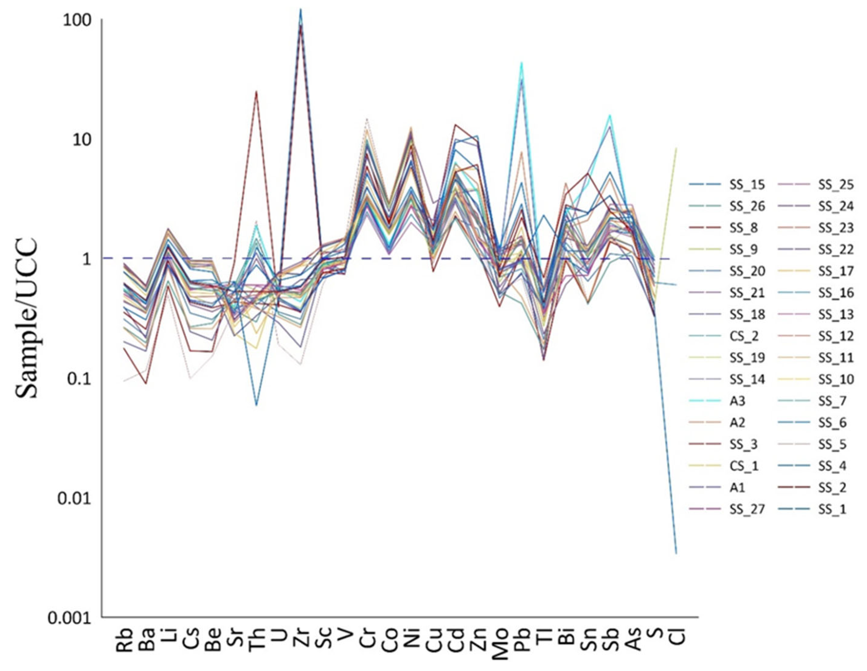
3.4.2. Trace Elements

The concentrations of 27 trace elements determined in the soil samples are shown in Table S2 along with the calculated minimum, maximum, average, and standard deviations. The average concentrations of trace elements in the study area were arranged in descending order: Cl >P > Cr > S > Ni > Ba > Zn > Sr > V > Zr > Pb > Rb > Cu > Co > Li > Sc > As > Sn > Cs > U > Sb > Be > Mo > Cd > TI > Bi. The overall highest concentration was obtained for Cl in SS19 (2.5 g kg−1). The second highest concentration in the studied soils was found for P (from 64.1 to 1168 mg kg−1), while the lowest concentrations were obtained for Bi (from below the limits of detection to 0.7 mg kg−1).

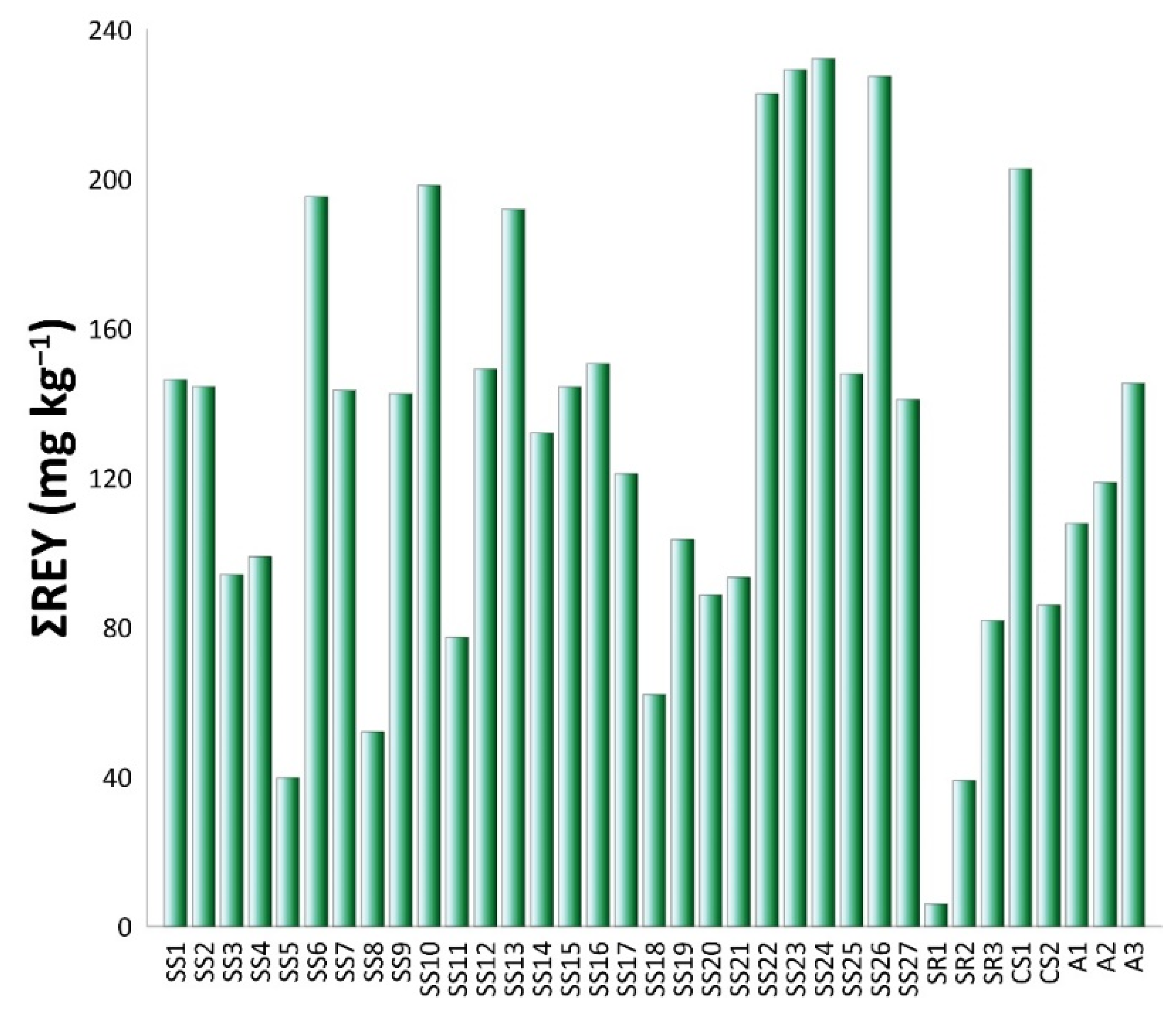
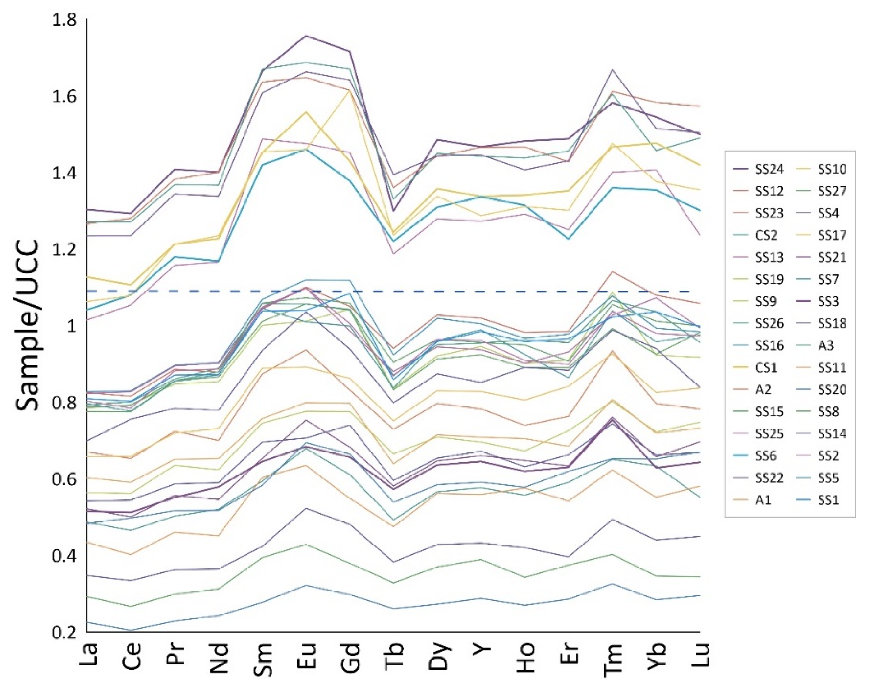
3.4.3. Rare Earth Elements (REEs)

The REE concentrations in 35 samples are listed in Table 5. A summary of the main statistical parameters (min, max, average, standard deviation, and RSD) is also given. The distribution of total LREE, HREE, REEs, and total REY-related calculated parameters, as well as the europium and cerium anomalies, (La/Yb)UCC, (La/Nd)UCC, and (Er/Nd)UCC are shown in Table 6. The concentrations of REEs in the analyzed samples ranged from 0.01–81.4 mg kg−1 (Table 5). Ce and La had the highest concentrations in all of the samples analyzed, while the concentrations of Tm and Lu were the lowest. The total ΣREEs ranged from 3.36 to 161 mg kg−1 (Table 6). The highest ΣREE concentrations were measured in sample SS24 (ΣREEs = 161 mg kg−1), the lowest were measured in sample SR1 (ΣREEs = 3.36 mg kg−1), while the concentrations of the total REEs + Y (ΣREY) ranged from 5.96 to 232 mg kg−1 in all of the analyzed samples. The lowest value of ΣLREE/ΣHREE was obtained for the source rock sample from site SR1 (ΣLREE/ΣHREE = 8.28), while the highest value was observed for the soil sample from site SS24 (ΣLREE/ΣHREE = 12.2). In all the samples, both anomalies showed a broader range of values, from 0.95 to 1.34 and from 0.76 to1.02 for Eu/Eu* and Ce/Ce*, respectively. The latter are the ratios of (La/Yb)UCC, (La/Nd)UCC, and (Er/Nd)UCC in the sediments, where (La/Yb)UCC ranged from 0.72 to1.16 with an average of 0.81, (La/Nd)UCC ranged from 0.86 to1.22 with an average of 0.93, and the ratios of (Er/Nd)UCC were higher than 1 in all samples (only one was less than 1), ranging from 0.99 to 1.69.
The total ΣREEs ranged from 3.36 to161 mg kg−1 (Table 6). The highest ΣREE concentrations were measured in sample SS24 (ΣREEs = 161 mg kg−1), the lowest were measured in sample SR1 (ΣREEs = 3.36 mg kg−1), and the concentrations of the total REEs + Y (ΣREY) ranged from 5.96 to 232 mg kg−1 in all of the analyzed samples. The lowest value of ΣLREE/ΣHREE was obtained for the source rock sample from site SR1 (ΣLREE/ΣHREE = 8.28), while the highest value was observed for the soil sample from site SS24 (ΣLREE/ΣHREE = 12.2). In all samples, both anomalies showed a broader range of values, from 0.95 to1.34 and from 0.76 to1.02 for Eu/Eu* and Ce/Ce*, respectively. The latter are the ratios of (La/Yb)UCC, (La/Nd)UCC, and (Er/Nd)UCC in the sediments, where (La/Yb)UCC ranged from 0.72 to1.16 with an average of 0.81, (La/Nd)UCC ranged from 0.86 to1.22 with an average of 0.93, and the ratios of (Er/Nd)UCC were higher than 1 in all samples (only one was less than 1), ranging from 0.99 to1.69.

4. Discussion

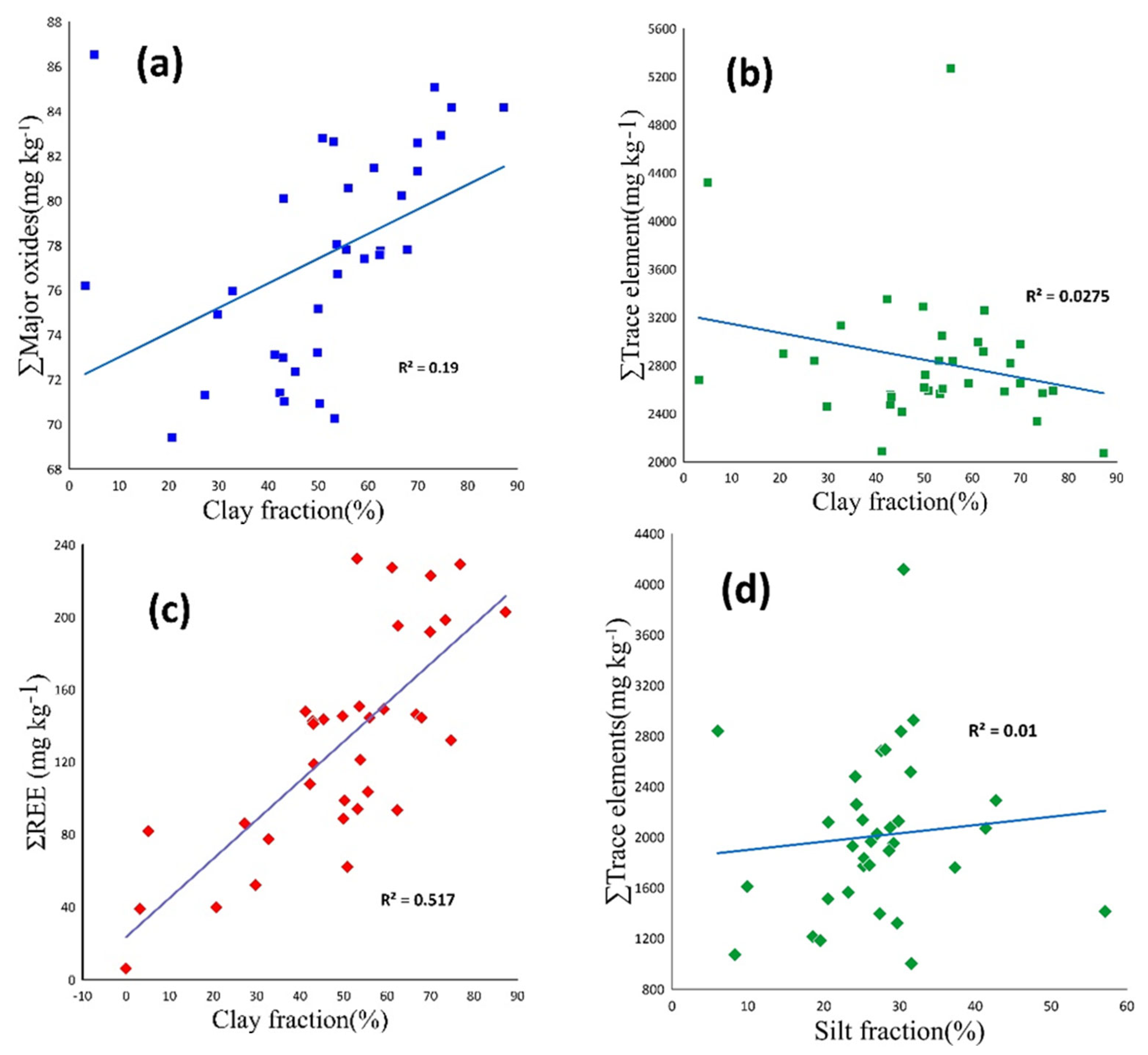
4.1. Grain Size Distribution of the Soil Samples

Grain size is one of the most important parameters affecting the ability of sediments to concentrate and retain metals [37]. There is usually a strong correlation between an increase in metal concentration and a decrease in grain size [38], and fine-grained particles are the most important for metal accumulation and transport due to their large specific surface area and cation exchange capacity [39]. As expected, the content of major oxides increased as the grain size decreased (Figure 3a, Table 2, Table 3 and Table 4), except for CaO. This is due to the fact that CaO, similar to quartz [40], is normally concentrated in the coarse-grained fraction. Similar to major elements, trace elements also increase with decreasing grain size in different soils [41]. However, in the studied samples, trace element concentrations and fine grain size are inversely correlated (Figure 3b, Table 2 and Table S2), with the exception of Th and Zr. Studies by Horowitz and Elrick [42] however, revealed an inverse correlation between trace metal concentrations and grain size. Because of their large surface area and high organic matter content, sediment particles metal concentrations increase when their size is reduced. Otherwise, trace element concentrations increased with increasing silt fractions (Figure 3d).
Due to the minerals present in the finest fraction, including accessory primary and secondary minerals, some immobile elements such as Al, Ti, Zr, Th, and REEs are typically concentrated in fine-grained sediments, as suggested by Soureiyatou et al. [43]. According to Laveuf and Cornu [44], clay minerals are the main factor affecting the distribution of REE in soils. In the present study, the regression analysis showed that ΣREEs tend to increase with increasing clay content in soils, as shown in Figure 3c. This is in agreement with the results of Rao et al. [45] and Gulcin and Alwasel [46], who found that the amount of REEs increases when the particle size decreases and when the proportion of clay components increases.

4.2. Organic Matter (OM) Distribution and pH in Soils

In order to investigate the relationship between the proportion of organic matter and the pH value with the element distribution in the soils, correlation coefficients were determined. As shown in Table 7, organic matter plays an important role in the distribution of the metals in the studied soils. The positive correlation between Al and K could be due to the high proportion of illite in the clay minerals ([47], Table 2). Most trace elements were also positively correlated with OM (r > 0.5; Table 7), while rare earths showed an even stronger correlation with OM, with correlation coefficients ranging from 0.63 to 0.67 (Table 7). Cao et al. [48] found that as soil pH increases, the bond strengths between rare earths and organic complexes become stronger [49].
The studied soils are neutral to moderately alkaline (pH between 7.35 and 9.92), which is due to the high content of carbonate, ash, and slag from anthropogenic sources, as well as to alkaline components in the atmosphere [50]. Soils with pH levels between 7.5 and 8.4 indicate the presence of free lime (CaCO3) in the soil, which usually provides excellent filtration and infiltration of water due to the high Ca content in clays. On the other hand, soils with a pH of >8.4 indicate calcareous soil associated with poor physical conditions, slow infiltration and percolation of soil water, possible root destruction, and the dissolution of organic matter [28]. Studies by [51] showed that higher pH values (pH > 8) were more common in younger sedimentary deposits than in older sedimentary deposits. In general, the statistical analysis in Table 7 shows that there is no significant correlation between the element concentrations and soil pH, except for Sr (r = 0.63), which has a strong positive relationship with pH. Sr concentrations are usually higher when the pH is between 7 and 8.5 [52].

4.3. Mineral Composition of the Soils

Table 2 and Table 3 show that the coarser the grain size, the more quartz occurs in the sand and silt fractions, and conversely clay minerals occur predominantly in fine clay fractions. The frequent occurrence of quartz is consistent with previous studies in the area [53]. Calcite is also present in large quantities in most of the soil samples (Table 3) and could be derived from the weathering of limestone during soil formation, which is the parent rock of the Sinjar Formation of the study area. Previous studies [54] suggest that the micritic groundmass in the Sinjar Formation is sometimes neomorphosed into coarse calcite crystals, as found in mud-dominated facies. Additionally, although many fossils are originally composed of the mineral aragonite, these grains convert to the more stable mineral calcite with time, as in all other areas of the formation [55]. In addition, all soil samples from the Kolosh Formation are characterized by a high content of serpentine minerals (Table 3). Serpentine is formed by serpentinization from olivine, pyroxene, and amphibole minerals [56,57]. Feldspars and clinochlor are generally associated with coarser grain sizes, and pyroxene occurs in all fractions (Table 3). In the Eocene formations, quartz, feldspars, parts of kaolinite, and illite are usually detrital minerals, and the formation of these minerals is caused by diagenesis with feldspars and montmorillonite as substrates for their formation [58]. Hematite and gypsum were found in sample SS27, gypsum was found in SS20, while these phases are absent in the other soil samples and in the source rock (Table 3). It is possible that they were formed elsewhere by deposition or wind transport. The results in Table 3 show that montmorillonite is predominant in all samples except SS7 and SR1. Illite is the second most abundant clay mineral in the samples studied, while chlorite was found as a rare clay mineral in sample SS15. The clay minerals and chlorite traces in the studied samples are consistent with previous findings that clay minerals in the Sulaimani region generally consist of montmorillonite, illite, palygorskite and traces of chlorite and kaolinite [59,60]. Palygorskite was found to have a fine grain size at 4 sample sites, which is consistent with its general occurrence in the clay fraction [61,62]. Montmorillonite and palygorskite are the main eogenetic clay minerals, while illite and chlorite are depositional, unlike the diagenetic clay minerals proposed by [63]. However, mineral analysis showed that SSP had no effect on the mineralogy of the soils in the study area, possibly due to the short period of establishment of the plant.

4.4. Distribution of Elements in Studied Samples

4.4.1. Major Oxides

The data on the major oxides are given in Table 4, while the calculated Pearson correlation coefficients and the UCC-normalized patterns are shown in Table 8. The Pearson correlation coefficients were calculated with the aim of gaining better insight into the origin of the major elements in the studied soils.
The SiO2 content shows a negative correlation with CaO and LOI and a positive correlation with TiO2, Al2O3, MnO, Fe2O3, and K2O (Table 8). The content of Na is lower than in UCC (Figure 4). The reason for this is the generally increased Na mobility during weathering and water transport, as indicated by Ref. [64]. The Al content was slightly lower than in UCC. In contrast, the Mg and Ca content is higher than in UCC (Figure 4), and CaO shows a negative correlation with SiO2, Al2O3, and TiO2 (Table 8), most likely due to the limestone deposits found almost everywhere in the area. As shown in Figure 4, the Ti content in the UCC values is generally slightly higher in the samples located downwind and close to the storage sites (i.e., SS6, SS10, SS13, SS14, SS22, SS23, SS24, SS26, and CS1). Additionally, the authors of Ref. [64] suggested that the high Ti content could be explained by the presence of numerous iron, steel, cement, and porcelain factories that make extensive use of titanium-bearing alloys or high-grade ceramics. The presence of the same feature in the case of Fe could also be due to industrial activities in the area. Namely, ferrotitanium alloys are used as raw materials in the steel industry [65]. This is also supported by the observed negative correlations between Fe2O3 and CaO, SiO2 and LOI, and Fe2O3 and LOI (Table 8).
Moreover, TiO2 and Al2O3 are refractory oxides that are highly resistant to weathering [66], and the Al2O3/TiO2 ratio in clastic sedimentary rocks can be used as an important tool to identify different types of source rocks. Studies by Ref. [67] suggest that the concentrations of Ti and Al can also change due to dilution by quartz, calcite, and other non-clay minerals, so it is better to use the ratio of these two resistant oxides as an indicator of origin. The Al2O3/TiO2 ratios in the studied samples, ranging from 11.6 to 19.8 (Table 4), indicate that these soils originated from mafic source rocks in the study area.

4.4.2. Trace Elements

The data on the concentrations of trace elements are presented in Table S2. Of the trace elements measured, Cl, P, Cr, Ni, V, Zn, Pb, Co, and As had the highest values of 765, 503, 493.7, 281, 100, 195, 59.2, 32.4, and 7.9 mg kg−1, respectively. The Cl content was higher in SS19, which may be due to either atmospheric deposition from industrial and municipal sources or directly from the use of animal wastes, which often have high chlorine content [68]. The high phosphorus concentration (Table S2) could be a consequence of the excessive use of fertilizers such as superphosphate in the area [18]. In addition, the soils near the steel plant had higher concentrations of Cr, V, Zn, Pb, Co, Ni, and As than other sites, similar to what Strezov and Chaudhary [6] reported for soils near steel plants in Australia. The UCC-normalized samples show that the studied samples are strongly enriched in Zn, Pb, Th, Sb, Cr, Ni, and Cd (Figure 5). In addition, a slight enrichment with As, Sn, Bi, V, Co, Li, Th and Cu is observed. The observed enrichments are consistent with previous findings on element distribution in the soils surrounding similar plants [11,13,14,15]. The minerals present may also promote the adsorption of certain elements. According to Uddin [69], montmorillonite has the ability to adsorb Cu, Pb, Hg, Cd, Zn, Ni, Co, Sr, Cs, and Cr, while illite readily adsorbs Pb, Cr, and Cd [47].

4.4.3. Rare Earth Elements

Descriptive statistics of the REEs concentration in studied soil samples are given in Table 5, while the calculated anomalies and fractionation indices are presented in Table 6. As can be seen from Table 6, two anomalies, europium and cerium were in a fairly narrow range. A slightly negative Ce anomaly and a positive Eu anomaly were also noted. Craigie [47] noted that a positive Eu anomaly is usually due to a high proportion of plagioclase feldspars in the parent rock of the soils. The sandstones of the Kolosh Formation could be a source of feldspars that release Eu and other elements through weathering and accumulate in the soils of the area. On the other hand, the slightly negative anomaly of Ce usually reflects oxic-suboxic environments because Ce is less easily dissolved under such conditions [47]. The calculated UCC-normalized patterns for selected elements, (La/Yb)UCC, (La/Nd)UCC, and (Er/Nd)UCC (Table 6) showed that the MREEs were significantly enriched compared to LREEs and HREEs, and that the HREEs were enriched compared to LREEs, which is consistent with the data reported for topsoil [49].
Figure 6 shows the spatial distribution of ΣREY in soil samples and parent rock. The highest ΣREY concentrations were measured in soil samples along the SS10, SS13, SS22, SS24, and SS26 wind directions with ΣREY concentrations of 198, 192, 223, 229, 232, and 228 mg kg−1, respectively. Wang and Lian [70] and Fiket et al. [71] also found that the content of the REE decreased with distance and was the highest along the prevailing wind direction. Soil sample SS6, which was taken closest to the nearby steel mill warehouse, had ΣREY of 195 mg kg−1.
The distribution of REEs in the studied samples, normalized to UCC, is shown in Figure 7. It shows a slight enrichment of HREE compared to LREE, which is consistent with the fractionation indices for REE in the studied samples (Table 6), i.e., a predominance of LREE (La-Gd) over HREE (Tb-Lu+Y) with ΣLREE/ΣHREE in the range of 8.28–12.2. The soils were characterized by a general predominance of elements from Sm to Gd, resulting in a convex shape of the normalized curve, similar to what was found by Fiket et al. [72] for soils in the vicinity of thermal power plant. Moreover, the distribution patterns of the REEs in the soil samples from the seven sampling sites SS6, SS10, SS13, SS22, SS24, SS23, and SS26 collected downwind were similar and showed enrichment. The fractionation of REEs in most soil samples was much higher than that of the bedrock and reference sample (CS2). Although CS1 was a reference soil sample, it was collected downwind and therefore has somewhat higher values (Figure 7).

4.5. Contamination Assessment

4.5.1. Enrichment Factor (EF)

The calculated EFs for trace element concentrations in the soils in the vicinity of SSP (Table S3) showed moderate enrichment with Th, V, Co, Cu, Zn, TI, Sb, and As near the factory and 300 m away from SSP, very high enrichment of Pb, Cr and Ni in the northeast and southeast directions at 100–300 m from SSP, and extremely high enrichment of Cr and Ni at 500 m and 1000 m in the northeast and southeast directions at 100 m from SSP.
Compared to the reference soil composition (Table S4), it was found at EF that the trace element concentrations in the soils surrounding the plant are moderately enriched with Sr, Th, P, Sc, Cr, Co, Ni, Cd, Cu, Zn, Mo, Pb, TI, Bi, As, S, Sn, and Sb within 500 m of SSP, are very high enriched with Cr at site SS5, and extremely highly enriched with Th within 500 m northeast of SSP, and with Pb in the soils surrounding the plant. The EF values determined here are consistent with literature values for soils near industrial and similar facilities [73,74,75], confirming the extremely high impact of the Sulaimani steel plant on the environment. The differences in the enrichments obtained using different reference materials are due to the fact that when local soils are used, their mean element concentrations are higher than the background values, which further confirms the widespread environmental impact of SSP.
Compared to the UUC [35], the EFs of the REE concentrations in soils (Table S5) near SSP showed moderate enrichment with Sm, Eu, Gd, and Tm, which also confirms the influence of SSP on rare earth element concentrations. All other rare earths elements showed minimal enrichment in all directions from SSP. The EFs of the REE concentrations in soils compared to the reference soil composition (Table S6), it was found minimal enrichment in all directions from SSP.

4.5.2. Geoaccumulation Index (Igeo)

The Igeo values for trace elements calculated with respect to the average global soil composition [34] and average reference soil composition are shown in Tables S7 and S8 respectively. Insight into the spatial variability of Igeo values is also provided, as shown in Figure 8 and discussed below. The Calculated Igeo values in the soil samples (Figure 8a, Table S7) based on the average world soil composition [34] around SSP classify the studied soils as uncontaminated to moderately contaminated with As; moderately contaminated with Co, Cu, Pb, and Sb; and moderately to heavily contaminated with Cr, Ni, and Zn. To the north of SSP, at a distance of 1000 m, based on Igeo, soils can be classified as uncontaminated to moderately contaminated with Th, V, Cu and As; moderately contaminated with Co, Zn and Tl; moderately to strongly contaminated with Cr and strongly contaminated with Ni. However, in the eastern direction of SSP, at a distance of 1000 m, soils can be classified as uncontaminated to moderately contaminated with Cu and V, moderately to heavily contaminated with Co, and heavily to extremely contaminated with Cr and Ni. The Calculated Igeo values of the soil samples in the west at 1000 m from SSP classify soils as uncontaminated to moderately contaminated with Sc, V, Cu, Zn, and As; moderately contaminated with Co, and heavily contaminated with Cr and Ni. The calculated Igeo values in the soil samples in the south at 1000 m from SSP classify soils as uncontaminated to moderately contaminated with V, Cu, Zn, Sb and As; moderately contaminated with Co and moderately to heavily contaminated with Cr and Ni. The average Igeo values in the southeast direction at 500 to 2000 m downwind from SSP describe soils as uncontaminated to moderately contaminated with Zn, As, and V; moderately contaminated with Co and Cu; moderately to strongly contaminated with Cr; and strongly contaminated with Ni. The average Igeo values in the southwestern direction at a distance of 500–2000 m from SSP describe the soils as uncontaminated to moderately contaminated with Sr, Th and Cu; moderately contaminated with Co; and moderately to strongly contaminated with Cr and Ni.
The Igeo values for trace elements, calculated based on the composition of the reference soils, showed that the soil in the vicinity of SSP is uncontaminated to moderately contaminated by Sb, Sn, Zn, Cd, Zr, Rb, Ba, Li, Cs, and Be (Igeo < 1) and moderately contaminated by Pb (Igeo <2). The average Igeo values were ranked as follows: Pb > Sb > Sn > Zn > Cd > Zr > Rb > Ba > Li > Cs > Be (Figure 8b, Table S8).
The results of the Igeo values of the studied REEs compared to the UUC [35] are shown in Figure 8c and in Table S9 and are based on the reference soil values of the sample (Figure 8d, Table S10). Compared to the UUC [35], the Igeo values of REE concentrations in soils near the plant’s warehouse and downwind at a distance of 1000–1500 m from SSP describe them as moderately to strongly contaminated with Dy and uncontaminated to moderately contaminated with Gd, Tb, and Y within and near the plant.

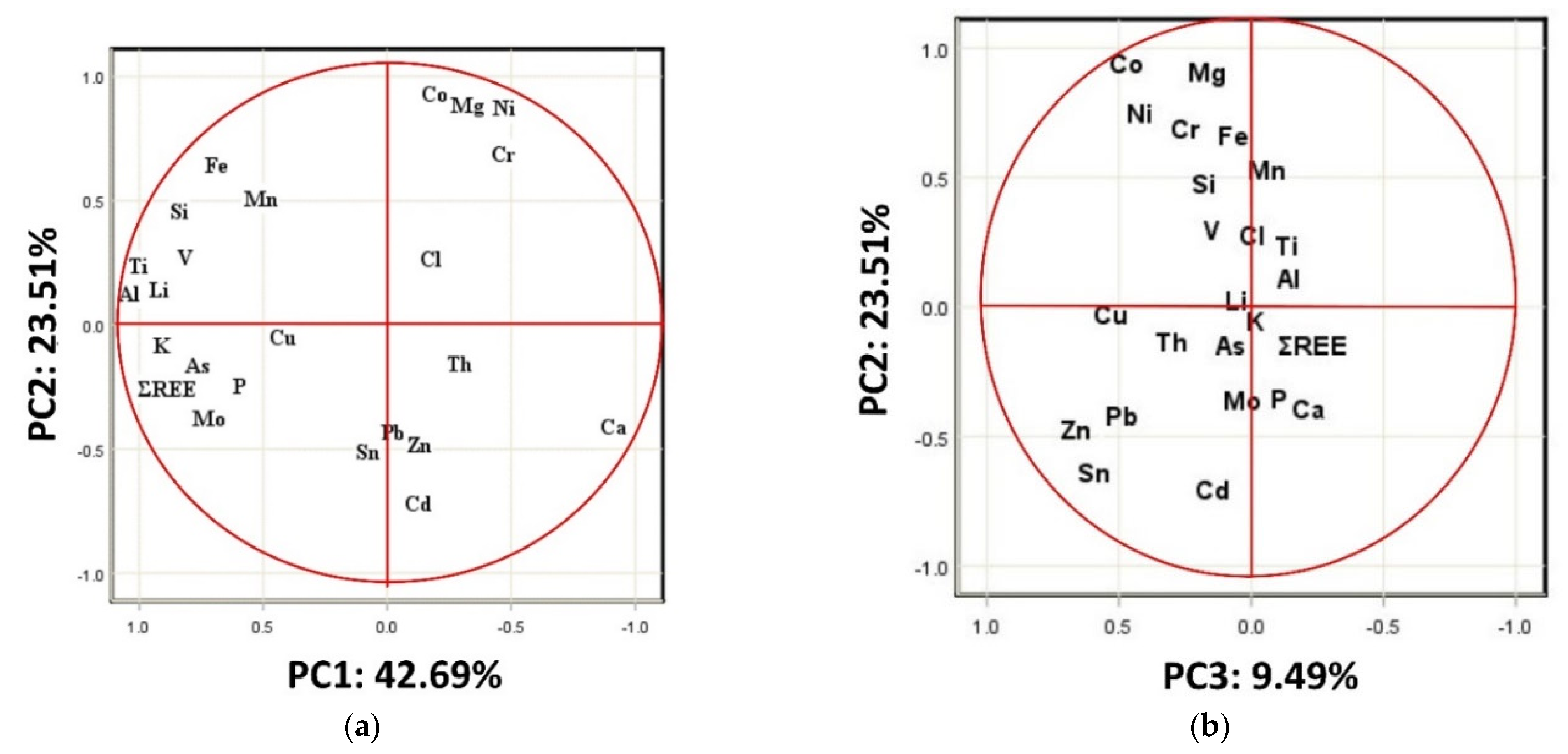
4.6. Principal Component Analysis (PCA)

To determine the sources controlling the element distribution in the studied soils, PCA was performed on the data set using concentrations of major and trace elements, including rare earths. The significance of the determined principal component factors was determined based on the calculated eigenvalues [76]. The first four PCs explained 82.0% of the total variability among the variables; the first component (PC1) contributed 42.7%, while the second (PC2), third (PC3), and fourth (PC4) components contributed 23.5, 9.5, and 6.3% of the total variance, respectively. The PCA factor loading for these first four PCs is shown in Table 9 and Figure 9. The Al, Li, K, Ti, and ∑REE had the highest positive PC1 loadings, while Ca had the highest negative PC1 loading, indicating that the composition of the soils is primarily determined by the geogenic sources, i.e., geochemistry of the background of the study area, which consists of carbonates and aluminosilicate minerals [77,78].
The Co, Cr, Mg, and Ni displayed the highest positive loading on PC2. Their common grouping indicates their common anthropogenic source. Khudhur et al. [31] previously reported elevated Cr, Co and Ni levels in soils near a steel plant in Erbil, while Reck et al. [79] reported that Ni is mainly used in alloyed form in a steel plant. Mg is also frequently found in elevated concentrations near steel mills because it is produced during iron and steel manufacturing [75]. For PC3, the highest positive loadings were found for Cu, Sn, Pb, and Zn, also suggesting their common origin. It is a group of elements originating from various anthropogenic sources, from transport to various industrial sources. Their separation from the other highly enriched elements in the soil around the Sulaimani steel plant suggests that they originate from somewhat different anthropogenic sources than those that primarily contribute to the high enrichment of Cr and Ni. This is also confirmed by the fact that the highest enrichments of the first and second groups of elements were not necessarily found in the same locations. Interestingly, Th exhibited the greatest influence on PC4, further confirming that the soils surrounding SSP are enriched in metals from multiple sources.

5. Conclusions

The geochemical features of the studied samples suggest that industrial activities at the Sulaimani Steel Plant (SSP) have led to the significantly high accumulation of heavy metals and rare earth elements (REE) in local soils. The latter is particularly emphasized downwind, highlighting their role in dispersing metal-rich particles from the steel plant into the environment. Elevated levels were observed for many elements, including Ti, Fe, Pb, Cr, Ni, Th, V, Co, Cu, Zn, TI, Sb, As, Sm, Eu, Gd and Tm, with the highest overall enrichment for Cr (EF up to 20.7), Ni (EF up to 14.2), Pb (EF up to 80.4) and Th (EF up to 50.4). Such enrichment levels indicate a high risk to soil and environmental health and potential adverse effects on human health, highlighting the need for continuous monitoring mechanisms and environmental management measures.

Supplementary Materials

The following are available online at https://www.mdpi.com/article/10.3390/soilsystems6040086/s1, Table S1: Coordinates of sampling sites in the study area (locations indicated in Figure 1c,d). coordinates of sampling sites; Table S2: Trace element composition (in mg kg−1) of the studied samples; Table S3: Enrichment factors (EF) for trace elements in studied samples calculated based on soil world average soil values [33] using Al as a reference element; Table S4: Enrichment factors (EF) for trace elements in studied samples calculated based on average values in reference soils (CS1 and CS2) using Al as a reference element; Table S5: Enrichment factors (EF) for rare earth elements in studied samples calculated based on UCC values [34] using Al as a reference element; Table S6: Enrichment factors (EF) for rare earth elements in studied samples calculated based on average values in reference soils (CS1 and CS2) using Al as a reference element; Table S7: Geoaccumulation indices (Igeo) for trace elements in studied samples calculated based on soil world average soil values [33]; Table S8: Geoaccumulation indices (Igeo) for trace elements in studied samples calculated based on average values in reference soils (CS1 and CS2); Table S9: Geoaccumulation indices (Igeo) for REEs in studied samples calculated based on UCC values [34]; Table S10: Geoaccumulation Index (Igeo) for REEs in studied samples calculated based on average values in reference soils (CS1 and CS2).

Author Contributions

Conceptualization, R.A.H. and I.M.J.M.; methodology, R.A.H. and Ž.F.; software, R.A.H.; formal analysis, R.A.H. and Ž.F.; investigation, R.A.H.; resources, R.A.H., I.M.J.M. and Ž.F.; data curation, R.A.H.; writing—original draft preparation, R.A.H.; writing—review and editing, I.M.J.M. and Ž.F.; visualization, R.A.H.; This paper is a part of the MSc thesis by the first author. All authors have read and agreed to the published version of the manuscript.

Funding

This study has been supported in part by Croatian Science Foundation under the project FORtIS (IP-2019-04-9354).

Institutional Review Board Statement

Not applicable.

Informed Consent Statement

Not applicable.

Data Availability Statement

Not available.

Conflicts of Interest

The authors declare no conflict of interest.

References

  1. Ebel, A.; Davitashvili, T. Air, Water and Soil Quality Modelling for Risk and Impact Assessment; Springer: Berlin/Heidelberg, Germany, 2007; pp. 29–44. [Google Scholar]
  2. Harrison, R.M. Principles of Environmental Chemistry; Royal Society of Chemistry: Cambridge, UK, 2007. [Google Scholar]
  3. Cullen, J.M.; Allwood, J.M.; Bambach, M.D. Mapping the Global Flow of Steel: From Steelmaking to End-Use Goods. Environ. Sci. Technol. 2012, 46, 13048–13055. [Google Scholar] [CrossRef] [PubMed]
  4. Allwood, J.M.; Cullen, J.M.; Milford, R.L. Options for Achieving a 50% Cut in Industrial Carbon Emissions by 2050. Environ. Sci. Technol. 2010, 44, 1888–1894. [Google Scholar] [CrossRef] [PubMed]
  5. Mocellin, J.; Mercier, G.; Morel, J.L.; Blais, J.F.; Simonnot, M.O. Factors influencing the Zn and Mn extraction from pyrometallurgical sludge in the steel manufacturing industry. J. Environ. Manag. 2015, 158, 48–54. [Google Scholar] [CrossRef] [PubMed]
  6. Strezov, V.; Chaudhary, C. Impacts of iron and steelmaking facilities on soil quality. J. Environ. Manag. 2017, 203, 1158–1162. [Google Scholar] [CrossRef]
  7. Lourenco, R.W.; Landim, P.M.B. Risk mapping of public health through geostatistics methods. Public Health Rep. 2005, 21, 150–160. [Google Scholar]
  8. Sethi, S.; Gupta, P. Soil Contamination: A Menace to Life; IntechOpen: London, UK, 2020. [Google Scholar] [CrossRef]
  9. Duckworth, O.W.; Polizzotto, M.L.; Thompson, A. Bringing soil chemistry to environmental health science to tackle soil contaminants. Front. Environ. Sci. 2022, 10, 981607. [Google Scholar] [CrossRef]
  10. Schulin, R.; Curchod, F.; Mondeshka, M.; Daskalova, A.; Keller, A. Heavy metal contamination along a soil transect in the vicinity of the iron smelter of Kremikovtzi (Bulgaria). Geoderma 2007, 140, 52–61. [Google Scholar] [CrossRef]
  11. Yuan, G.L.; Sun, T.H.; Han, P.; Li, J. Environmental geochemical mapping and multivariate geostatistical analysis of heavy metals in top soils of a closed steel smelter: Capital Iron & Steel Factory, Beijing, China. J. Geochem. Explor. 2013, 130, 15–21. [Google Scholar]
  12. Mohiuddin, K.; Strezov, V.; Nelson, P.F.; Stelcer, E.; Evans, T. Mass and elemental distribution of atmospheric particles nearby blast furnace and electric arc furnace operated industrial areas in Australia. Sci. Total Environ. 2014, 487, 323–334. [Google Scholar] [CrossRef]
  13. Akporido, O.S.; Agbaire, O.P.; Ipeaiyeda, R.A. Effect of steel production on the quality of soil around udu section of Warri river in the vicinity of a steel plant, Nigeria. Asian J. Appl. Sci. 2014, 7, 552–567. [Google Scholar] [CrossRef] [Green Version]
  14. Namuhani, N.; Kimumwe, C. Soil Contamination with Heavy Metals around Jinja Steel Rolling Mills in Jinja Municipality, Uganda. J. Health Pollut. 2017, 5, 61–67. [Google Scholar] [CrossRef] [PubMed]
  15. Ladonin, V.D. Lanthanides in Soils of the Cherepovets Steel Mill Impact Zone. Eurasian Soil Sci. 2017, 50, 672–680. [Google Scholar] [CrossRef]
  16. Mohialdeen, I.M.J.; Luqman, O.; Hamasalih, L.O.; Schwark, L. Geochemistry of a crude oil from a shallow well in Bazian Area, Sulaimani, Kurdistan Region, NE Iraq. J. Zankoy Sulaimani Part A 2013, 15, 3. [Google Scholar] [CrossRef]
  17. Rasheed, R.O.; Faqesaleh, L.I. Evaluation of some heavy metals from water and soil of Bazian Oil Refinery within Sulaimani Governorate, IKR. Marsh Bull 2016, 11, 123. [Google Scholar]
  18. AL-Taay, A.S.M.; Al-Assie, A.H.A.; Rasheed, O.R. Impact of Bazian Cement Factory on Air, Water, Soil, And Some Green Plants in Sulaimani City-Iraq. Iraqi J. Agric. Sci. 2018, 1027, 354–366. [Google Scholar]
  19. Ahmed, T.H. Groundwater Potential Mapping and Wellhead Protection Areas in Bazian Sub-Basin, Sulaimani, Kurdistan Region, Iraq. Ph.D. Thesis, University of Sulaimani, Sulaimani, Iraq, 2020. [Google Scholar]
  20. Hamakarim, B.M. Environmental Evaluation of Some Heavy Metals and Background Radiation Pollution in Soils around the Scrap Metal Recycling Factories in Sulaimani Governorate-Iraq. Ph.D. Thesis, University of Sulaimani, Sulaimani, Iraq, 2020; 137p. [Google Scholar]
  21. Jassim, S.Z.; Guff, J.C. Geology of Iraq; Jassim, S.Z., Ed.; Directorate General for Geological Survey and Mineral Investigations Publication: Brno, Czech Republic, 2006; 445p. [Google Scholar]
  22. Hamamin, D.F. Hydrogeological Assessment and Groundwater Vulnerability Map of Basara Basin, Sulaimani Governorate, Iraqi Kurdistan Region. Ph.D. Thesis, University of Sulaimani, Sulaymaniyah, Iraq, 2011; 227p. [Google Scholar]
  23. Ahmad, K.H.K. Facies Changes Between Kolosh and Sinjar Formations Along Zagros Fold–Thrust Belt in Iraqi Kurdistan Region. J. Geogr. Geol. 2016, 8, 1. [Google Scholar]
  24. Fiket, Ž.; Mikac, N.; Kniewald, G. Mass Fractions of Forty-Six Major and Trace elements, including Rare Earth Elements, in Sediment and Soil Reference Materials used in Environmental Studies. Geostand. Geoanalytical Res. 2016, 41, 123–135. [Google Scholar] [CrossRef]
  25. D422–63 ASTM; Standard Test Method for Particle-Size Analysis of Soils. ATSM International: West Conshohocken, PA, USA, 2014.
  26. D854–14 ASTM; Standard Test Methods for Specific Gravity of Soil Solids by Water Pycnometer. ATSM International: West Conshohocken, PA, USA, 2014.
  27. El-Wakeel, S.K.; Riley, J.P. The Determination of Organic Carbon in Marine Muds. ICES J. Mar. Sci. 1957, 22, 180–183. [Google Scholar] [CrossRef]
  28. Estefan, G.; Sommer, R.; Ryan, J. Methods of Soil, Plant, and Water Analysis: A Manual for the West Asia and North Africa Region, 3rd ed.; ICARDA (International Center for Agricultural Research in the Dry Areas): Beirut, Lebanon, 2013. [Google Scholar]
  29. Muller, G. Index of geoaccumulation in sediments of the Rhine River. Geol. J. 1969, 2, 108–118. [Google Scholar]
  30. Ridgway, J.; Shimmield, G. Estuaries as Repositories of Historical Contamination and their Impact on Shelf Seas. Estuar. Coast. Shelf Sci. 2002, 55, 903–928. [Google Scholar] [CrossRef]
  31. Khudhur, N.S.; Khudhur, S.H.M.; Ahmad, I.N. An Assessment of Heavy Metal Soil Contamination in a Steel Factory and the Surrounding Area in Erbil. Jordan J. Earth Environ. Sci. 2018, 9, 1–11. [Google Scholar]
  32. Loska, K.; Wiechuła, D.; Barska, B.; Cebula, E.; Chojnecka, A. Assessment of arsenic enrichment of cultivated soils in Southern Poland. Pol. J. Environ. Stud. 2003, 12, 187–192. [Google Scholar]
  33. Muller, G. Die Schwermetallbelstung der sediment des Neckars und seiner Nebenflusse: Eine Bestandsaufnahme. Chem. Zeitung. 1981, 105, 156–164. [Google Scholar]
  34. Kabata-Pendias, H.A.; Mukherjee, A.B. Trace Elements from Soil to Human; Springer: Berlin/Heidelberg, Germany, 2007; ISBN 13 978-3-540-32713-4. [Google Scholar]
  35. Rudnick, R.L.; Gao, S. Composition of the Continental Crust. In Treatise on Geochemistry; Rudnick, R.L., Holland, H.D., Turekian, K.K., Eds.; Elsevier: Amsterdam, The Netherlands, 2003; Volume 3, pp. 1–64. [Google Scholar]
  36. USDA (U.S. Department of Agriculture). Keys to Soil Taxonomy, 10th ed.; USDA: Washington, DC, USA, 2006; p. 332. [Google Scholar]
  37. Maslennikova, S.; Larina, N.; Larin, S. The effect of sediment grain size on heavy metal content. Lakes Reserv. Ponds 2012, 6, 43–54. [Google Scholar]
  38. Huang, B.; Yuan, Z.; Li, D.; Zheng, M.; Nie, X.; Liao, Y. Effects of soil particle size on the adsorption, distribution, and migration behaviors of heavy metal(loid)s in soil: A review. Environ. Sci. Process. Impacts 2020, 22, 1596–1615. [Google Scholar] [CrossRef] [PubMed]
  39. Al-Swadi, H.A.; Usman, A.R.A.; Al-Farraj, A.S.; Al-Wabel, M.I.; Ahmad, M.; Al-Faraj, A. Sources, toxicity potential, and human health risk assessment of heavy metals-laden soil and dust of urban and suburban areas as affected by industrial and mining activities. Sci. Rep. 2022, 12, 8972. [Google Scholar] [CrossRef]
  40. Mirza, A.T. Composition and phase mineral variation of Portland cement in Mass Factory Sulaimani–Kurdistan Region NE-Iraq. Int. J. Basic Appl. Sci. 2012, 12, 109–118. [Google Scholar]
  41. Al-Khuzie, D.K.; Al-Hatem, Z.; Shabar, H.A.; Hassan, W.F.; Abdulnabi, Z.A. Heavy metal distribution in grain size fraction in surface sediments: Pollution assessment of Iraqi Coasts. Eco. Env. Cons. 2021, 27, S388–S398. [Google Scholar]
  42. Horowitz, E.; Elrick, K. The relation of stream sediment surface area, grain size and surface area to trace element chemistry. Appl. Geochem. 1987, 2, 437–451. [Google Scholar] [CrossRef]
  43. Soureiyatou, F.D.; Chavom, M.B.; Paul-désiré, N. Trace and rare earth elements (REE) distribution in Ngaye alluvial sediments of Mbere-Djerem Basin, North Cameroon: Implications for origin, depositional conditions and paleoclimate reconstitution. SN Appl. Sci. 2020, 2, 2054. [Google Scholar] [CrossRef]
  44. Laveuf, C.; Cornu, S. A review on the potentiality of rare earth elements to trace pedogenetic processes. Geoderma 2009, 154, 1–12. [Google Scholar] [CrossRef]
  45. Rao, W.; Tan, H.; Jiang, S.; Chen, J. Trace element and REE geochemistry of fine- and coarse-grained sands in the Ordos deserts and links with sediments in surrounding areas. Geochemistry 2011, 71, 155–170. [Google Scholar] [CrossRef]
  46. Gulcin, I.; Alwasel, S.H. Metal Ions, Metal Chelators and Metal Chelating Assay as Antioxidant Method. Processes 2022, 10, 132. [Google Scholar] [CrossRef]
  47. Craigie, N. Principles of Elemental Chemostratigraphy. In Advances in Oil and Gas Exploration & Production; Springer: Berlin/Heidelberg, Germany, 2018. [Google Scholar] [CrossRef]
  48. Cao, X.; Chen, Y.; Wang, X.; Deng, X. Effects of redox potential and pH value on the release of rare earth elements from soil. Chemosphere 2001, 44, 655–661. [Google Scholar] [CrossRef]
  49. Zhang, Q.; Han, G.; Liu, M.; Wang, L. Geochemical Characteristics of Rare Earth Elements in Soils from Puding Karst Critical Zone Observatory, Southwest China. Sustainability 2019, 11, 4963. [Google Scholar] [CrossRef] [Green Version]
  50. Al Obaidy, A.M.J.; Al Mashhadi, A.A.M. Heavy metal contaminations in urban soil within Baghdad City, Iraq. J. Environ. Prot. 2013, 4, 72–82. [Google Scholar] [CrossRef] [Green Version]
  51. Kazlauskaitė-Jadzevičė, A.; Volungevičius, J.; Gregorauskienė, V.; Marcinkonis, S. The role of PH in heavy metal contamination of urban soil. J. Environ. Eng. Landsc. Manag. 2014, 22, 311–318. [Google Scholar] [CrossRef]
  52. Yu, S.; Liu, Y.; Pang, H.; Tang, H.; Wang, J.; Zhang, S.; Wang, X. Chapter 1—Novel nanomaterials for environmental remediation of toxic metal ions and radionuclides. In Emerging Nanomaterials for Recovery of Toxic and Radioactive Metal Ions from Environmental Media; Wang, X., Ed.; Elsevier: Amsterdam, The Netherlands, 2022; pp. 1–47. [Google Scholar] [CrossRef]
  53. Al-Hakari, S.H.S. Geometric Analysis and Structural Evolution of NW Sulaimani Area, Kurdistan Region, Iraq. Ph.D. Thesis, University of Sulaimani, Sulaimanyah, Iraq, 2011; 309p. [Google Scholar]
  54. Salih, A.L.M. Sedimentology of Sinjar and Khurmala Formations (Paleocene-Lower Eocene) in Northern Iraq. Ph.D. Thesis, University of Baghdad, Baghdad, Iraq, 2013; 215p. [Google Scholar]
  55. Flugel, E. Microfacies of Carbonate Rocks, 2nd ed.; Springer: Berlin, Germany, 2010; p. 976. [Google Scholar]
  56. Sadiq, D.M. Geochemistry and Geochronology of Detrital Heavy Minerals in Cretaceous Flysch and Cenozoic Molasse of the Northeastern Iraq. Ph.D. Thesis, University of Sulaimani, Sulaimani, Iraq, 2020; 142p. [Google Scholar]
  57. Folk, R.L. Petrology of Sedimentary Rocks; Hemphill Publishing Company: Austin, TX, USA, 1974; 182p. [Google Scholar]
  58. Smirnov, P.; Deryagina, O.; Afanasieva, N.; Rudmin, M.; Gursky, H.-J. Clay Minerals and Detrital Material in Paleocene–Eocene Biogenic Siliceous Rocks (Sw Western Siberia): Implications for Volcanic and Depositional Environment Record. Geosciences 2020, 10, 162. [Google Scholar] [CrossRef]
  59. Mohialdeen, I.M.J.; Merza, T.A. Composition and Origin of White Carbonate Layer in Seramerg-Tagaran area, Sulaimani, Ne Iraq. Zanko 2004, 16, 17–23. [Google Scholar]
  60. Mohialdeen, I.M.J.; Merza, T.A. Manufacture of Brick Tiles from Local Raw Materials, N & NE Iraq. J. Zankoy Sulaimani 2005, 8, 31–45. [Google Scholar]
  61. Al-Tamimi, R.A.K.H. Identifying of Clay Minerals in Some Iraqi Soils. Ph.D. Thesis, University of Baghdad, Baghdad, Iraq, 1984. [Google Scholar]
  62. Al-Obaidi, B.S. Natural Occurance of Palygorskite in Some Iraqi Gypsiferous Soils. Ph.D. Thesis, University of Baghdad, Baghdad, Iraq, 2008. [Google Scholar]
  63. Worden, R.H.; Morad, S. Clay Minerals in Sandstones: Controls on Formation, Distribution and Evolution. Int. Assoc. Sedimentol. Spec. Publ. 2003, 34, 3–4. [Google Scholar] [CrossRef]
  64. Badawy, W.; Ghanim, E.; Duliu, O.; El Samman, H.; Frontasyeva, M. Major and trace element distribution in soil and sediments from the Egyptian central Nile Valley. J. Afr. Earth Sci. 2017, 131, 53–61. [Google Scholar] [CrossRef]
  65. Takeda, O.; Ouchi, T.; Okabe, T.H. Recent Progress in Titanium Extraction and Recycling. Met. Mater. Trans. A 2020, 51, 1315–1328. [Google Scholar] [CrossRef]
  66. Hill, I.; Worden, R.; Meighan, I. Geochemical evolution of a palaeolaterite: The Interbasaltic Formation, Northern Ireland. Chem. Geol. 2000, 166, 65–84. [Google Scholar] [CrossRef]
  67. Andersson, P.; Worden, R.; Hodgson, D.; Flint, S. Provenance evolution and chemostratigraphy of a Palaeozoic submarine fan-complex: Tanqua Karoo Basin, South Africa. Mar. Pet. Geol. 2004, 21, 555–577. [Google Scholar] [CrossRef]
  68. Geilfus, C.-M. Chloride in soil: From nutrient to soil pollutant. Environ. Exp. Bot. 2018, 157, 299–309. [Google Scholar] [CrossRef]
  69. Uddin, M.K. A review on the adsorption of heavy metals by clay minerals, with special focus on the past decade. Chem. Eng. J. 2017, 308, 438–462. [Google Scholar] [CrossRef]
  70. Wang, L.; Liang, T. Geochemical fractions of rare earth elements in soil around a mine tailing in Baotou, China. Sci. Rep. 2015, 5, 12483. [Google Scholar] [CrossRef] [Green Version]
  71. Fiket, Z.; Medunic, G.; Kniewald, G. Rare earth element distribution in soil nearby thermal power plant. Environ. Earth Sci. 2016, 75, 598. [Google Scholar] [CrossRef]
  72. Fiket, Ž.; Mikac, N.; Kniewald, G. Influence of the geological setting on the REE geochemistry of estuarine sediments: A case study of the Zrmanja River estuary (eastern Adriatic coast). J. Geochem. Explor. 2017, 182, 70–79. [Google Scholar] [CrossRef]
  73. Sidhu, G.P.S.; Bali, A.S.; Singh, H.P.; Batish, D.R.; Kohli, R.K. Insights into the tolerance and phytoremediation potential of Coronopus didymus L. (Sm) grown under zinc stress. Chemosphere 2020, 244, 125350. [Google Scholar] [CrossRef] [PubMed]
  74. Alfaro, M.R.; Ugarte, O.M.; Lima, L.H.V.; Silva, J.R.; da Silva, F.B.V.; Lins, S.A.D.S.; Nascimento, C.W.A.D. Risk assessment of heavy metals in soils and edible parts of vegetables grown on sites contaminated by an abandoned steel plant in Havana. Environ. Geochem. Health 2022, 44, 43–56. [Google Scholar] [CrossRef] [PubMed]
  75. Zhou, T.; Bo, X.; Qu, J.; Wang, L.; Zhou, J.; Li, S. Characteristics of PCDD/Fs and metals in surface soil around an iron and steel plant in North China Plain. Chemosphere 2018, 216, 413–418. [Google Scholar] [CrossRef] [PubMed]
  76. Issa, H.M.; Alshatteri, A.H. Source Identification, Ecological Risk and Spatial Analysis of Heavy Metals Contamination in Agricultural Soils of Tanjaro Area, Kurdistan Region, Iraq. UKH J. Sci. Eng. 2021, 5, 18–27. [Google Scholar] [CrossRef]
  77. Soltani-Gerdefaramarzi, S.; Ghasemi, M.; Ghanbarian, B. Geogenic and anthropogenic sources identification and ecological risk assessment of heavy metals in the urban soil of Yazd, central Iran. PLoS ONE 2021, 16, e0260418. [Google Scholar] [CrossRef]
  78. Fiket, Z.; Mlakar, M.; Kniewal, G. Distribution of Rare Earth Elements in Sediments of the Marine Lake Mir (Dugi Otok, Croatia). Geosciences 2018, 8, 301. [Google Scholar] [CrossRef] [Green Version]
  79. Reck, B.K.; Müller, D.B.; Rostkowski, K.; Graedel, T.E. Anthropogenic Nickel Cycle: Insights into Use, Trade, and Recycling. Environ. Sci. Technol. 2008, 42, 3394–3400. [Google Scholar] [CrossRef]
Figure 1. (a) Location of Kurdistan Region in Iraq, (b) location map of the studied samples, (c) sampling sites at different distances from the Sulaimani Steel Plant (SSP), (d) sampling sites downwind from the SSP to a distance of 2000 m in the direction of SE.
Soilsystems 06 00086 g001
Figure 2. Classification of the studied surface soil samples according to their grain size. (After diagram; USDA, 2006 [36]).
Soilsystems 06 00086 g002
Figure 3. Correlation coefficients according to Pearson between different element groups, the main oxides (a), the trace elements (b,d), the rare earths (c) and the clay or silt content in soil.
Soilsystems 06 00086 g003
Figure 4. Upper-Continental Crust (UCC) normalized major oxide diagram for the studied samples.
Soilsystems 06 00086 g004
Figure 5. Upper-Continental Crust (UCC) normalized trace elements diagram for the studied samples.
Soilsystems 06 00086 g005
Figure 6. Spatial distribution of ΣREEs in soil samples (A1–A3; SS1–SS27), source rocks (SR1–SR3), and reference soils (CS1 and CS2).
Soilsystems 06 00086 g006
Figure 7. Upper-Continental Crust (UCC) normalized REEs patterns for the studied samples.
Soilsystems 06 00086 g007
Figure 8. Igeo for trace elements and REEs calculated based on average world soil data ((a,c) respectively) or average values in reference soils ((b,d) respectively).
Soilsystems 06 00086 g008
Figure 9. PCA loadings plots: (a) PC1 vs. PC2, (b) PC2 vs. PC3.
Soilsystems 06 00086 g009
Table 1. Instrumental conditions of the HR ICP-MS and data acquisition parameters for determination of selected elements.
ParametersHR ICP-MS Operating Conditions
RF power:1200 W
Coolant Ar flow:15.5 L min−1
Auxiliary Ar flow:0.85 L min−1
Sample gas flow rate:1.063 L min−1
Torch:Fassel type, 1.5 mm i.d.
Nebulizer:Micro Mist, AR40-1-F02, 0.2 mL min−1 (Glass Expansion)
Spray chamber:Twister, 50 mL, Cyclonic (Glass Expansion)
Sample cone:Ni, 1.1 mm aperture i.d.
Skimmer cone:Ni, 0.8 mm aperture i.d.
Acquisition mode:E-scan
No. Scans:20 (5 runs, 4 passes)
Resolution:low (LR) = 300
medium (MR) = 4000
high (HR) = 10,000
Calibration:External
Table 2. Granulometric characteristics and physicochemical properties, organic matter (OM), and pH value in studied samples.
Sample% Sand% Silt% ClayOMpH
A125.931.842.37.97.4
A227.029.943.19.37.7
A320.130.249.83.47.9
SS18.125.366.72.28.9
SS28.323.867.91.68.9
SS317.529.253.22.48.9
SS28.323.867.91.68.9
SS317.529.253.22.48.9
SS425.524.350.21.68.9
SS547.731.620.70.38.7
SS69.927.662.57.58.2
SS728.426.245.48.58.6
SS840.529.729.81.88.7
SS915.741.442.96.28.3
SS101.325.373.45.58.4
SS1139.927.432.75.18.5
SS1214.726.059.26.58.3
SS134.925.169.97.88.2
SS144.820.674.66.38.3
SS1517.027.056.05.38.4
SS1618.328.153.74.68.7
SS1717.628.653.82.38.9
SS1830.618.650.81.59.0
SS1913.930.555.61.98.8
SS2030.519.650.01.28.7
SS2114.423.262.33.18.3
SS225.924.270.09.38.0
SS232.620.676.86.58.0
SS244.242.753.17.58.1
SS2521.537.341.25.48.5
SS267.431.561.18.68.3
SS2728.228.843.05.88.8
CS12.99.987.24.67.7
CS215.757.127.24.47.9
SR1___0.59.9
SR288.68.33.20.49.4
SR388.96.05.12.78.4
Average22.027.051.04.68.5
Table 3. Quantitative mineral composition of fraction < 2 mm of the investigated samples.
Non Clay Minerals (%)Clay Minerals (%)
SampleCalQSerFelClinPyHeGyChaDoMagMonIllPalChl
A151.813.54.4--------15.510.2--
A248.717.0---------20.912.4--
A311.713.5---------26.610.7--
SS127.316.8---------28.514.012.2-
SS223.725.314.06.6-------29.0 --
SS353.018.9--7.7------11.68.2--
SS460.413.6---------15.210.0--
SS557.913.3---------24.33.5--
SS612.321.1--------9.023.917.119.0-
SS741.116.9----------12.628.4-
SS849.314.26.111.6-------17.7---
SS938.57.9--17.311.1-----10.313.6--
SS10-25.79.4--------42.016.9--
SS1129.925.928.0--------8.07.5--
SS1226.623.1---10.8-----23.215.2--
SS134.819.09.3--------43.117.7--
SS14-31.2---------40.212.314.6-
SS1532.123.7-16.4-------21.5--4.1
SS1630.926.7---8.1-----12.616.0--
SS1737.116.59.8--------15.712.6--
SS1839.914.0---------46.0---
SS1921.813.717.06.3-------35.9---
SS2027.83.517.0--12.0--8.2--31.0---
SS2131.020.014.9--------26.06.8--
SS22-19.76.5--18.0-----34.120.1--
SS234.817.04.8--------45.120.8--
SS2414.321.0---------42.218.1--
SS2549.114.0---------22.213.3--
SS2620.514.5--5.84.6-----32.420.5--
SS2744.911.9-19.6--3.50.5---18.1---
CS1-11.6-8.212.3------67.0---
CS251.78.9---------30.47.2--
SR194.72.5-------1.6-----
SR237.93.134.6--------20.92.7--
SR3-13.636.3--------38.010.7--
Ca: Calcite, Q: Quartz, Ser: Serpentine, Fel: Feldspar, Cli: Clinochlore, Py: Pyroxene, He: Hematite, Gy: Gypsum, Cha: Chapazite, Do: Dolomite, Mag: Magnesiohoreblende, Mont: Montmorillonite, Ill: Illite, Paly: Palygorskite, Chl: Chlorite. -: (no quantitative value is assigned to -) not determined.
Table 4. Major oxides (wt.%) concentrations of the soils and source rocks in the study area.
SampleSiO2Al2O3Na2OMgOK2OTiO2MnOCaOP2O5Fe2O3SO3LOITotalAl2O3/TiO2
A126.75.770.072.550.990.340.0831.20.133.390.2128.499.817.0
A228.76.590.092.891.120.370.0727.30.113.510.2528.899.817.8
A334.18.230.132.821.140.500.0922.00.163.940.1826.399.516.5
SS141.99.560.115.481.260.660.1215.30.105.600.1519.599.714.5
SS241.39.130.076.111.120.680.1213.20.105.800.2121.799.513.4
SS326.16.050.043.380.740.340.0629.70.093.780.0129.699.917.8
SS424.15.670.022.510.910.320.0533.80.093.370.0828.999.817.7
SS522.83.560.015.950.320.180.0632.40.073.820.1630.499.819.8
SS645.112.10.043.801.510.930.157.50.176.390.1421.899.613.0
SS729.97.860.133.021.150.440.0725.60.123.870.2027.599.917.9
SS825.66.800.212.110.700.540.1433.60.194.690.2825.099.912.6
SS931.08.690.083.461.230.460.0824.00.243.580.1926.999.918.9
SS1052.215.20.064.111.531.250.182.490.137.820.1314.899.812.2
SS1133.65.310.0112.20.680.340.0918.60.104.940.1123.799.715.6
SS1239.29.120.084.721.380.610.1116.60.115.340.2022.499.815.0
SS1348.714.30.064.061.601.110.175.340.147.090.0417.199.712.9
SS1451.211.60.046.561.111.000.192.950.148.030.1016.899.811.6
SS1539.28.221.125.841.290.540.1019.70.104.360.1922.1102.615.2
SS1638.89.160.203.691.450.590.0919.20.334.360.1421.899.915.5
SS1735.67.540.105.161.170.480.0921.70.114.730.0723.199.815.7
SS1834.95.440.0610.80.560.350.0825.10.075.370.0816.999.715.5
SS1936.97.110.049.121.060.490.1017.40.105.440.0421.799.514.5
SS2034.16.090.018.900.740.420.1019.40.085.300.0724.699.814.5
SS2138.46.970.018.140.980.480.0916.30.105.900.1422.299.814.5
SS2249.313.40.144.421.820.990.164.040.166.540.3218.599.813.6
SS2349.815.30.084.181.891.130.173.720.147.640.1515.799.813.6
SS2448.014.50.134.311.641.050.165.280.177.040.4517.199.813.8
SS2529.58.080.142.601.200.480.0827.10.143.720.0326.899.916.8
SS2647.013.50.154.041.861.070.176.760.206.620.0718.499.812.7
SS2733.09.040.133.331.250.520.0928.10.194.170.2219.899.917.4
CS150.615.40.063.881.391.110.163.540.097.880.0715.599.713.9
CS226.95.020.073.600.660.320.0630.30.113.990.2228.599.815.7
SR12.500.040.010.350.010.020.0153.50.010.830.1342.599.92.00
SR228.22.960.0418.50.250.190.2621.20.044.490.0123.599.715.6
SR345.67.640.0116.30.970.710.086.560.098.530.0913.299.810.8
Average36.38.600.115.511.110.600.1119.20.135.200.1522.999.814.3
Table 5. Rare earth element composition (in mg kg−1) of the studied samples.
SampleYLaCePrNdSmEuGdTbDyHoErTmYbLu
SS120.725.150.66.1823.54.881.044.330.603.730.792.220.312.070.31
SS220.224.949.46.2623.94.901.104.020.613.760.752.070.311.960.30
SS313.516.032.23.9115.63.030.682.620.402.480.511.450.231.260.20
SS414.116.834.34.1615.93.270.712.960.422.550.521.520.221.320.21
SS56.036.9712.91.626.541.300.321.190.181.060.220.660.100.570.09
SS628.132.368.08.3731.56.671.465.510.855.101.092.820.412.710.40
SS720.824.748.96.0723.54.911.014.000.593.740.771.990.311.910.30
SS88.179.0516.82.128.421.850.431.520.231.440.280.860.120.690.11
SS919.924.349.96.0223.04.701.014.170.583.590.752.090.331.850.28
SS1027.032.967.98.6133.36.831.466.450.875.221.092.990.442.750.42
SS1111.713.525.33.2712.22.830.632.190.332.190.481.250.191.100.18
SS1221.425.651.46.2923.74.911.104.200.664.010.822.260.342.160.33
SS1326.731.466.48.2131.56.991.485.810.834.991.072.870.422.810.38
SS1417.921.747.65.5621.04.391.043.760.563.410.742.030.301.880.26
SS1520.124.449.96.0723.74.981.074.230.633.760.792.090.322.020.31
SS1621.125.652.26.3624.45.021.124.470.653.970.802.250.321.990.31
SS1717.420.441.55.1119.74.170.893.450.533.240.671.930.281.650.26
SS189.110.821.02.579.841.990.521.920.271.670.350.910.150.880.14
SS1914.617.535.44.5116.83.500.783.100.472.760.561.670.241.440.23
SS2012.415.031.33.6714.02.740.692.660.382.280.481.420.201.300.21
SS2113.916.231.53.9514.73.070.752.730.412.520.541.460.231.310.22
SS2230.438.377.89.5436.17.551.666.560.985.631.173.290.503.030.47
SS2330.839.380.69.8137.87.691.656.460.955.621.223.280.483.160.49
SS2430.840.481.410.037.87.821.766.860.915.791.233.420.473.090.46
SS2519.725.552.16.3524.34.931.103.940.623.680.752.140.312.140.31
SS2630.339.480.09.7136.97.851.696.680.935.651.193.350.482.910.46
SS2719.424.048.86.0723.44.751.064.160.583.560.742.050.301.850.30
SR11.591.001.450.200.850.160.040.190.030.190.040.120.020.060.01
SR27.427.5412.01.365.381.060.331.090.151.100.240.630.090.540.08
SR311.715.127.63.2712.92.640.672.190.352.120.451.300.201.320.19
CS128.134.969.78.6133.16.821.565.720.875.291.113.110.442.950.44
CS212.115.129.33.5714.02.790.682.440.342.210.461.360.201.270.17
A114.918.737.24.6217.63.560.803.190.452.790.581.580.241.440.23
A216.420.841.15.1418.94.110.943.330.513.110.611.750.281.590.24
A320.024.650.46.1124.04.971.064.170.613.700.802.200.322.070.30
Min1.591.001.450.200.850.160.040.190.030.190.040.120.020.060.01
Max30.840.481.410.037.87.851.766.860.985.791.233.420.503.160.49
Average18.222.345.05.5221.24.390.983.780.553.370.701.950.291.800.27
SD7.619.8320.632.549.632.020.421.720.241.450.310.830.120.790.12
RSD41.744.245.945.945.646.143.245.544.243.043.542.741.744.143.4
Table 6. Calculated anomalies and fractionation indices for REEs in studied samples.
Sample∑REEs∑REY∑LREE∑HREE∑LREE/∑HREEEu/Eu *Ce/Ce *(La/Yb)UCC(La/Nd)UCC(Er/Nd)UCC
SS110114611610.011.50.980.960.780.931.11
SS299.41441149.811.71.070.930.820.911.01
SS364.794.274.16.511.41.050.960.820.891.09
SS468.199.078.16.811.50.980.970.820.921.12
SS526.739.830.82.910.71.120.900.790.931.18
SS613519515413.411.51.040.970.770.891.05
SS798.01431139.611.80.990.940.830.910.99
SS834.952.140.23.710.81.110.900.840.941.20
SS998.41431139.512.00.990.970.850.921.07
SS1013819815813.811.40.950.950.770.861.05
SS1152.177.359.95.710.51.100.900.790.961.20
SS1210214911710.611.11.050.950.760.941.12
SS1313419215213.411.41.000.970.720.871.07
SS1492.51321059.211.51.111.020.740.901.13
SS1599.91441149.911.51.010.970.780.891.03
SS1610415111910.311.61.020.960.830.921.08
SS1783.412195.28.5511.11.020.960.800.901.15
SS1842.262.148.64.3611.21.160.940.790.951.09
SS1971.510481.67.3711.11.020.940.780.901.16
SS2061.388.770.06.2611.21.121.000.740.931.20
SS2163.493.572.96.6810.91.130.930.790.961.16
SS2215422317715.111.81.020.960.810.921.07
SS2315922918315.212.11.010.970.800.901.02
SS2416123218615.412.11.040.950.840.931.06
SS2510314811810.011.91.080.960.770.911.03
SS2615822818215.012.21.010.960.870.931.07
SS2797.61411129.3812.01.030.950.840.901.03
SR13.365.963.890.478.280.990.761.161.021.69
SR224.139.028.82.8210.21.340.890.901.221.37
SR355.181.964.35.9210.91.210.920.741.021.18
CS114020316014.211.31.080.950.760.921.10
CS258.886.067.96.0111.31.130.940.770.931.14
A174.310885.77.3011.71.030.940.840.921.05
A281.611994.38.1011.61.100.940.840.961.09
A310114511510.011.51.010.970.770.891.08
min3.365.963.890.478.280.950.760.720.860.99
max16123218615.412.21.341.021.161.221.22
avg89.71301038.9411.31.060.940.810.930.93
stdev40.858.246.83.860.700.080.040.070.060.06
RSD45.544.745.443.26.207.084.389.026.516.51
ΣREE—sum of all rare earth element concentrations without Y element; ΣREY—sum of all rare earth element concentrations with Y element; ΣLREE/ΣHREE—ratio of sum of light rare earth and heavy rare earth element concentrations; Eu/Eu *—europium anomaly (Eu/Eu * = EuUCC/(SmUCC × GdUCC)); Ce/Ce *—cerium anomaly (Ce/Ce * = CeUCC/(LaUCC × PrUCC)0.5); (La/Yb)UCC—ratio of normalized La and Yb concentrations; (La/Nd)UCC—ratio of normalized La and Nd concentrations; (Er/Nd)UCC—ratio of normalized Er and Nd concentrations.
Table 7. Pearson’s correlation coefficients between major oxides, trace and rare earth elements and organic matter (OM) and pH in studied soil samples (N = number of samples).
N = 32SiO2Al2O3Na2OMgOK2OTiO2MnOCaOP2O5Fe2O3SO3LOI
OM0.390.530.10−0.370.670.470.38−0.400.380.220.35−0.22
PH−0.23−0.33−0.010.33−0.34−0.30−0.250.26−0.09−0.17−0.350.04
N = 32RbBaLiCsBeSrThUZrPScVCrCo
OM0.690.700.580.670.69−0.43−0.040.650.640.630.430.49−0.46−0.35
PH−0.54−0.52−0.49−0.53−0.500.63−0.25−0.45−0.49−0.41−0.52−0.540.130.02
N = 32NiCuCdZnMoPbTIBiSnSbAsSCl
OM−0.530.330.09−0.080.710.120.100.210.130.240.560.26−0.21
PH0.22−0.550.06−0.05−0.59−0.44−0.06−0.28−0.34−0.51−0.50−0.280.19
N = 32LaCePrNdSmEuGdTbDyYHoErTmYbLu
OM0.660.660.660.650.670.660.640.650.660.650.650.630.670.630.63
PH−0.40−0.39−0.39−0.38−0.39−0.41−0.37−0.38−0.38−0.38−0.39−0.39−0.41−0.41−0.38
Table 8. Pearson’s correlation coefficients for major oxides in studied samples.
SiO2Al2O3Na2OMgOK2OTiO2MnOCaOP2O5Fe2O3SO3
SiO21
Al2O30.889 **1
Na2O0.0860.0801
MgO0.164−0.232−0.1141
K2O0.7940.909 **0.205−0.3191
TiO20.9060.973 **0.039−0.1350.837 **1
MnO0.671 **0.612 **0.0090.3060.426 *0.669 **1
CaO−0.980 **−0.855 **−0.006−0.255−0.740 **−0.887 **−0.72 **1
P2O50.335 *0.467 **0.132−0.365 *0.599 **0.382 *0.151−0.2621
Fe2O30.925 **0.777 **−0.0960.3230.585 **0.857 **0.675 **−0.936 **0.1311
SO30.0630.1910.206−0.357 *0.2570.139−0.026−0.0190.317−0.0261
LOI−0.927 **−0.759 **−0.065−0.361 *−0.637 **−0.790 **−0.65 **0.890 **−0.268−0.91 **0.003
** Correlation is significant at the 0.01 level (2-tailed). * Correlation is significant at the 0.05 level (2-tailed).
Table 9. PCA factor loadings for elements in studied samples.
Components
Metals1234
Li0.970.090.01−0.07
Th−0.23−0.220.380.77
P0.63−0.28−0.150.23
V0.860.230.110.27
Cr−0.410.760.320.26
Co−0.130.870.400.07
Ni−0.420.820.360.00
Cu0.49−0.110.61−0.01
Cd−0.06−0.790.23−0.39
Zn−0.07−0.550.60−0.43
Mo0.78−0.440.120.05
Pb−0.02−0.500.570.23
Sn0.14−0.570.67−0.12
As0.83−0.220.010.22
Cl−0.120.210.07−0.38
Si0.890.410.12−0.05
Al0.980.06−0.08−0.02
Mg−0.260.820.25−0.20
K0.96−0.13−0.060.02
Ti0.950.17−0.07−0.08
Mn0.570.450.02−0.20
Ca−0.85−0.47−0.130.08
Fe0.740.580.15−0.13
ΣREEs0.97−0.15−0.090.04
Eigenvalue10.255.652.281.51
% Total Variance42.723.59.496.27
Cumulative %
Variance
42.766.275.782.0
PCA factor loadings > 0.6 are presented in bold.
Publisher’s Note: MDPI stays neutral with regard to jurisdictional claims in published maps and institutional affiliations.

