Abstract
The freeze–thaw process controls several hydrologic processes, including infiltration, runoff, and soil erosion. Simulating this process is important, particularly in cold and mountainous regions. The Soil and Cold Regions Model (SCRM) was used to simulate, study, and understand the behavior of twelve homogenous soils subject to a freeze–thaw process, based on meteorological data at a snow-dominated forest site in Laramie, WY, USA, from 2010 and 2012. The relationships of soil pore size, soil particle contact, and meteorological data were varied. Our analysis of the model compared simulations using metrics such as soil frost depth, days with ice, and maximum ice content. The model showed that the freeze–thaw process was strongest in the period with a shallow snowpack, with particle packing within the soil profile being an important factor in this process; that soil texture and water content control soil thermal properties; and that water movement towards the freezing front was especially important in fine-textured soils, where water and ice were concentrated in the upper layers. Based on these results, future research that combines a broader set of soil conditions with an extended set of field meteorology and real soil data could elucidate the influence of soil texture on the thermal properties related to soil frost.
1. Introduction
Frozen soils are an important factor that can control hydrologic processes such as meltwater infiltration, runoff timing and amount, water retention characteristics, and soil erosion [1,2,3,4]. When the ambient temperature reaches the soil’s freezing point, the freeze–thaw (FT) phenomenon plays an important role and is of interest to fields such as hydrology [5], engineering [6], agriculture [7], and forestry [8]. The FT process is especially relevant in cold regions, particularly at high elevations, where the influence of lower temperatures can result in more frequently frozen soils. These regions where seasonal soil frost is present are commonly located above 30° N–S [8]. This permeable/semipermeable ice layer can have regional effects on hydrologic response and soil thermal characteristics [9,10].
The phase change within the soil from water to ice and vice versa is controlled mainly by the movement of liquid water towards the freezing front, a process similar to water movement when the soil is drying [11,12,13,14]. Characteristics of a decrease in temperature in frozen soils can include decreased hydraulic conductivity [15] and increased water viscosity [16]. Therefore, coupling water and heat flow is necessary to predict the FT process [17].
One-dimensional (1D) numerical models have been used for decades to understand and describe soil freeze–thaw processes and soil–plant–atmosphere interactions, e.g., the CoupModel (Coupled heat and mass transfer Model for soil–plant–atmosphere systems) [18], SHAW (Simultaneous Heat and Water Model) [19], the SCRM (Soil and Cold Regions model) [20,21], and the spatially distributed ParFlow-CLM [22]. Nevertheless, the SCRM is currently the most comprehensive model, considering both meteorological data and vegetation properties.
One of the main factors controlling soil frost is the timing and amount of snowfall [23,24,25]. Freezing progresses from the ground surface downwards. Snow cover/soil (insulation ability) and cold weather intensity and timing control how deep-frozen soils occur [26,27,28]. Snowpack is an excellent thermal insulator due to its low thermal properties [29,30,31] and can insulate the soil from meteorological conditions such as cold weather [32,33]. Hence, the snowpack controls the duration and depth of the frozen layers within a soil [34], but this phenomenon is also controlled by other factors such as soil properties, precipitation patterns, and temperature.
Soil texture is an important factor controlling thermal processes in freezing soils [35,36,37]. Frozen soils control not only water infiltration into soil, but also runoff during spring [38,39]. Several studies have related freeze–thaw processes to soil texture [40,41,42,43]. The scope of previous research is restricted to a specific or local context, and does not present a broader framework required for universal analysis.
Understanding how soils behave under different weather scenarios will explain some of the hydrological processes described above. High elevation regions where soils freeze during the whole or part of a winter season [1] are dispersed worldwide, and the timing of snow melt is crucial for regional water availability. A lot of work worldwide has been dedicated to analyzing the freeze–thaw processes but focusing on specific sites and soils [44], in synthetic made soils [45], and in laboratory tests [13,46]. Despite the importance of the freeze–thaw processes, there has been little work to examine soil behavior in alpine zones using a wide range of soil types and their effect on the freeze–thaw processes. In this study, we provide a comprehensive and academic assessment of the freeze–thaw processes across a wide range of soil types in two contrasting climatic conditions. This analysis was performed by addressing the following research questions: (1) Is soil texture a major driver of the freeze–thaw process? (2) How do soil hydraulic properties function as a secondary driver of the freeze–thaw process?
We hypothesize that soil particle size, soil water content, and depth of snowpack directly influence the buildup of ice. Specifically, fine-textured soils, thinner snowpack, and higher soil water content will correlate with greater buildup of ice within the soil. This study also introduces metrics that aim to explain the behavior of different soil types in the presence of freeze–thaw processes. While these hypotheses are known, the main goal of this study was to synthesize the understanding of soil frost on different soil textures within contrasting climate input data. We intend this study to be a contribution and a guide to the development of research on the subject in areas where freezing processes have not been studied extensively, such as in South America.
2. Materials and Methods
Twelve soil textures were analyzed using the Soil in Cold Regions Model (SCRM) [20]. Section 2.1 describes the study site, its parameters of interest for the model, the sources of meteorological data, as well as the configurations and theory behind the SCRM model. Section 2.2 describes the metrics and assumptions used to evaluate the model’s performance.
2.1. Study Site, Meteorological Data, and Model Configuration
2.1.1. Study Site
A snow-dominated forest site located in the Medicine Bow National Forest (41°22′30.0″ N 106°15′30.5″ W, about 50 km west of Laramie, WY, USA) was chosen to drive the model. The site is at 3000 m elevation, south-facing, with a slope of 12.5° and is dominated by conifers, specifically Picea engelmannii Parry ex. Engelm. (Engelmann Spruce) and Abies lasiocarpa (Hook.) Nutt. (Subalpine fir). The parameters were defined in terms of vegetation as follows: average tree height = 20 m, stand stem biomass = 12 kg m−2, maximum stand Leaf Area Index (LAI) = 5 m2 m−2, and root mass = 4.4 kg m−2 [20].
2.1.2. Meteorological Dataset
For the model, we used meteorological data from study [20] for two hydrologic years (2010–2011 and 2011–2012). The data used in the model are described in [20,47]. The meteorological data were derived from a GLEES (Glacier Lakes Ecosystems Experiments Sites) tower from 5 to 15 min intervals. Rainfall (and snow) was collected from a rain gauge also at GLEES. The data utilized in the model were relative humidity (%), air temperature (°C), wind speed (m s−1), atmospheric pressure (Pa), precipitation (m), cloud cover fraction (dimensionless), atmospheric turbidity (dimensionless), leaf area index (m2 m−2), and stem area index (m2 m−2). Additionally, the wavelength (m), bandwidth (m), extraterrestrial radiation (J m−2 sm−1), water vapor absorption (1 m−1), ozone absorption (1 m−1), and miscellaneous gas optical depths were required to calculate incoming solar radiation at the Earth’s surface.
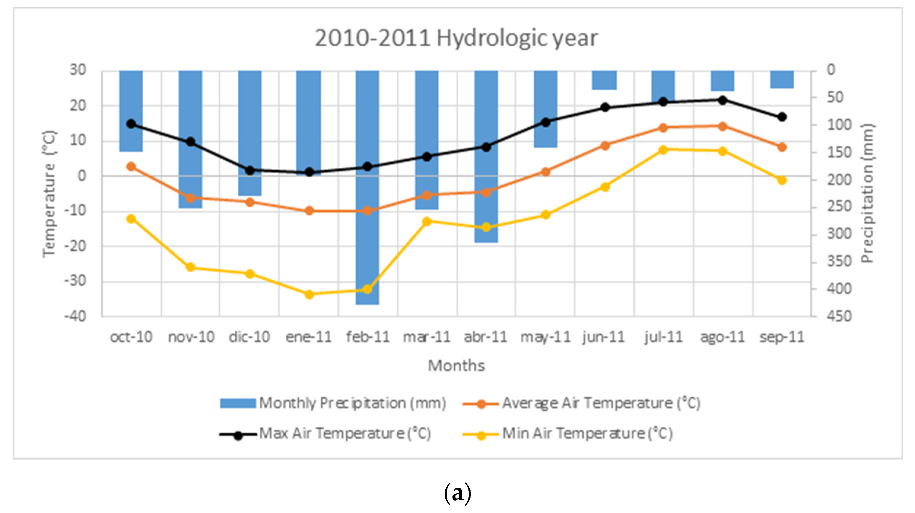
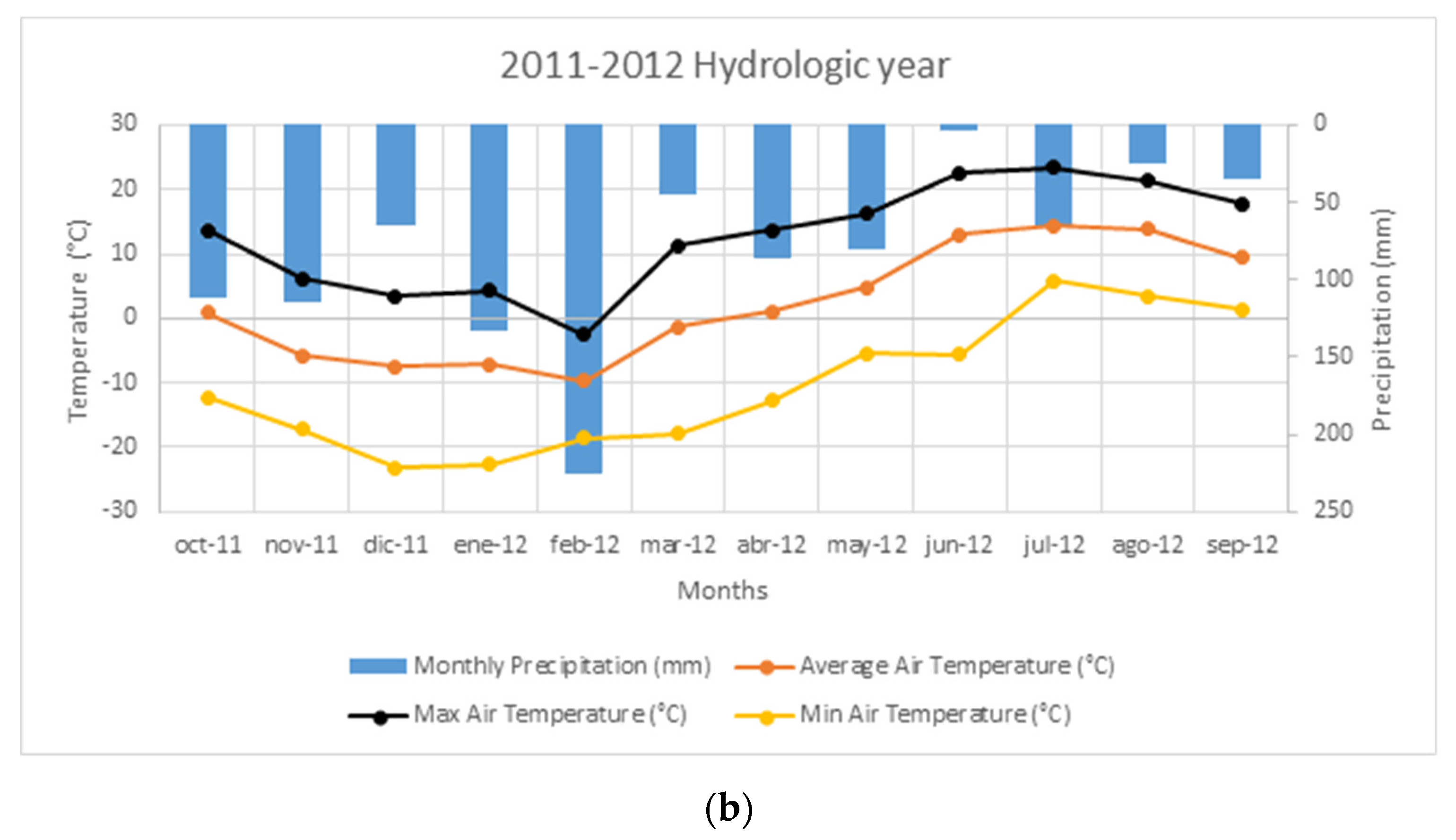
The monthly average precipitation and temperature distribution (Figure 1) in the 2010–2011 hydrologic year were characterized by temperatures ranging from −33.5 °C to 21.7 °C (0.6 °C average) and annual total precipitation of 2128 mm. The 2011–2012 hydrologic year was warmer and with less precipitation than 2010–2011. The temperature ranged from −23.24 °C to 23.39 °C (2.25 °C average) and annual total precipitation was 989 mm.


Figure 1.
Monthly precipitation (mm) and monthly average, min, and max air temperature (°C) for both hydrologic years 2010–2011 ((a), upper plot) and 2010–2012 ((b), lower plot).
2.1.3. Model Configuration
The Soil and Cold Regions Model (SCRM) is a one-dimensional numerical model that couples water flow and heat transport in soil and snow using all three phases of water: liquid, vapor, and ice [20,21]. The model is driven by precipitation and the surface energy balance at the top boundary and free drainage water flow, and zero temperature gradient for heat transport at the bottom. SCRM is physics-based and requires few empirical parameters. The model can deal with canopy–ground surface energy balance and root water uptake. The SCRM model is based on five main physical processes:
- Snow water flow, which depends on gravity (water) and temperature gradient (vapor).
- Soil water flow, which depends on the pressure head gradient, temperature gradient, and gravity (ignored for water vapor).
- Snow–soil heat transport, which is based on the convection and conduction. The model represents bulk snow–soil heat capacity, latent heat of vaporization, latent heat of fusion, snow–soil thermal conductivity, liquid water heat capacity, water vapor heat capacity, liquid water gravity, and water vapor flux.
- Soil–plant–atmosphere transfer, which is based on the canopy and ground surface energy balance. Here, evaporation is in terms of liquid and vapor water flow (at the upper half of the soil profile), and the water vapor heat transfer at the canopy.
- Root water uptake, which is a sink term within the soil water flow equation. This sink term is based on macroscopic root analysis.
The model does not include preferential flow, 2D or 3D processes, solute concentration changes, or changes in organic matter content. The main governing equations are described below and the mathematical derivation of the equations describing the entire process can be found in [20,21].
Soil water flow and snow–soil heat transport are described by Equations (1) and (2), respectively:
where t is time (s), is liquid water content (m3 m−3), is soil air relative humidity (dimensionless),is saturated water vapor density (kg m−3), is air content (m3 m−3), is ice density (kg m−3),is liquid water density (kg m−3),is ice content (m3 m−3), z is vertical coordinate (m),is isothermal liquid water hydraulic conductivity (m s−1), h is soil water pressure head (m),is thermal liquid water hydraulic conductivity (m2 s−1 K−1),is isothermal water vapor hydraulic conductivity (m s−1), is thermal water vapor hydraulic conductivity (m2 s−1 K−1), is root water uptake sink term (s−1), C is the soil heat capacity (J m−3 K−1), T is temperature (°C),is latent heat of vaporization (J kg−1),is latent heat of fusion (J kg−1), κ is soil thermal conductivity (J m−1 s−1 K−1),is liquid water heat capacity (J m−3 K−1), is liquid water flux (m s−1), is water vapor heat capacity (J kg−1 K−1), and is water vapor flux (expressed as an equivalent liquid water flux in m s−1). Note that = 1 for snow and 0 < < 1 for soil.
The energy balance equation can be expressed as:
In Equation (3), it should be noted that is set to zero and T is solved according to [48].
The model profile configuration holds 81 nodes ranging from 0.01 to 10.0 m deep. The van Genuchten–Mualem (vG) parameterization model was used to calculate the vG parameters for 12 soils (Figure 2 and Table 1). The ideal soils represent the basic 12 soil textures: sandy, loamy sand, sandy clay loam, sandy loam, sandy clay, loam, clay loam, clay, silty loam, silty clay loam, silty clay, and silt. The vG parameters were extracted using the Pedotransfer Function ROSETTA [49] and soil textures (sand, clay, and silt %) as input. Each texture was chosen randomly but setting up the criteria to be closer to the center of the soil type in the USDA soil triangle (red stars in Figure 2). It should be noted that at the model soil profile, the first 0.6 m of soil comprises layers 1 to 60 (0.01 m each), while the final (bottom) describes the remaining 9.4 m (node 61 to 81).
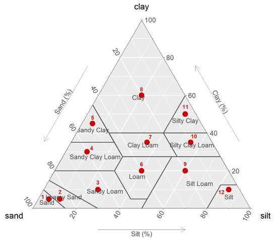
Figure 2.
Soil texture distribution. Each red circle represents the chosen soil texture to be used in the model (soils 1 to 12 in Table 1) (Figure was build using the ggtern R-package v2.2.0).

Table 1.
Soil texture distribution and vG parameters. Each soil number matches those in Figure 2.
2.2. Data Processing and Metrics Definition
The initial soil conditions (water content and temperature per node) were measured by [20] and then used as initial conditions in the model. The model includes two logic restrictions when it calculates the soil water pressure head, which are θ ≥ and ; both inequalities are physically based. Using the soil matric potential (MP) in the following way ensured that both statements are false. First, the initial water content was translated to pressure head values according to the van Genuchten equation and solving for suction pressure or matric potential (h).
Several metrics were developed to differentiate the behavior of the 12 soil textures:
- (i)
- Freeze–thaw cycles (FTCs) within a soil is when the ice water content (θi, in m3 m−3) goes above zero θi and then comes back again to zero. It was calculated as the number of annual cycles for each of the 12 soils.
- (ii)
- Maximum ice content measures the maximum ice content within the node. The first (0.01 m) and second (0.02 m) nodes were used to compute this metric because the maximum ice content can be found at these two depths.
- (iii)
- Total elapsed time (days/hours) where each soil had frost (i.e., days with ice). This value was computed within the first 5 nodes (0.01 to 0.05 m depth). It is important to note that this metric accounts for both continuous and discontinuous ice content.
- (iv)
- Temporal ice mass was calculated from the area under the curve of the ice mass time series, using the trapezoidal approximation method.
- (v)
- Maximum frost depth in each soil texture was defined as the last non-zero value within the soil profile.
3. Results
3.1. Snowfall Amount and Timing
In terms of snowfall, the first snowfall event differed between hydrologic years. In 2011–2012, it happened 20–30 days before that in 2010–2011, most likely because temperatures were lower in the first 5 days of the 2011–2012 hydrologic year compared to the previous hydrologic year. The snowpack behaviors in both hydrologic years were different. The 2010–2011 hydrologic year had a maximum snow depth of 4.64 m, whereas the 2011–2012 hydrologic year had a maximum snow depth of 1.99 m. The model did not show important differences in snowpack and Snow Water Equivalent (SWE) areas (days*m) between soil textures (Table 2). The difference in snow depth area was 14 days*m and 9 days*m and a SWE difference of 5.6 and 2.8 days*m for 2010–2011 and 2011–2012 hydrologic years, respectively.
Table 2.
Snow height and snow water equivalent (SWE) areas for both hydrologic years and all soils.
Minimal differences were found among each soil texture in terms of snow depth and SWE, as calculated by the model. In the 2010–2011 hydrologic year, the maximum snow depth difference was 4.4 cm and 1.7 cm for Snow Water Equivalent (SWE), while the 2011–2012 hydrologic year saw 3.7 cm for snow depth and 0.97 cm for SWE. Nevertheless, substantial differences were seen in the amount of snow, which is primarily due to higher precipitation levels and lower temperatures of the 2010–2011 hydrologic year.
3.2. Freeze–Thaw Metrics
3.2.1. Freeze and Thaw Cycles (FTCs)
The FTCs in the first 5 cm within the soil profile show significant variability across soil types (Table 3). Coarse soils such as sand and loamy sand had between one and three cycles in both periods. These values were the lowest within all 12 soil types, whereas the fine-textured soils such as clay and silt had a higher number of cycles.
Table 3.
Freeze and thaw cycles within first 5 cm depth (first five soil nodes) and maximum ice content in both hydrologic years (Hy) analyzed.
3.2.2. Maximum Ice Content
The maximum ice content is typically between 1 and 2 cm depth (Table 3). In general, the 2010–2011 hydrologic year holds the highest values of max ice content within all soil textures. In regard to soil texture ice content, silt texture held higher ice content at the upper soil in both hydrologic years.
A special case is the silt soil in the 2011–2012 hydrologic year, where the ice content goes up within the soil profile. This situation occurred in the spring season when the snow begins to melt, between January and late May, and a water refreezing event occurred, yielding infiltration. At 5 cm depth, a peak of water content occurs and remains constant until 40 cm depth; therefore, in response to cold temperatures, water in the upper part of the soil profile freezes.
3.2.3. Days with Ice
Similar to the FTCs, colder temperatures translate to more days with ice (Table 4). The very coarse and very fine-textured soils resulted in the most days with ice (Table 4; sand, loamy sand, and silt family soils). Interestingly, in the coarse soils, the highest volumetric ice content values were between 2 and 3 cm depth. This contrasts with the other soils, where freezing occurs within 1 cm depth. Loamy sand soil had the most days with ice during both periods due to its water content, as compared with sandy soil.
Table 4.
Days with ice and temporal ice mass metrics for both hydrologic years analyzed within the first 5 cm depth (first five soil nodes).
3.2.4. Temporal Ice Mass
Unlike the other metrics, temporal ice mass becomes evident within the first 5 cm depth (Table 4). The model computed the total, average, and maximum temporal ice mass per soil profile, and the mass ratio between the total and the maximum ice content. The temporal ice mass is concentrated between 1 and 2 cm depth, and the depth of the largest temporal ice areas is around 8 cm. The coarse soils have the greatest temporal ice mass in the upper layers, which is caused by water suction from lower layers and the capacity to hold more water than the other soils (low initial soil water content). On the contrary, fine-textured soils have a diminished ability to suck up water due to less pore availability and a higher initial soil water content.
3.2.5. Frost Depth
Coarse textured soils, such as sand and loamy sand, had the deepest soil frost among the soils. The fine-textured soils (sandy loam, sandy clay, and clay) had a shallower frost depth (Table 5). In general, the colder period (2010–2011) has deeper frost depth than the warmer period (2011–2012). However, some exceptions were found. Sandy clay and clay went down to only 14 cm depth, and they had some of the lowest FTCs in the 2010–2011 period, yet the same soils in the 2011–2012 period had a higher frost depth. One explanation is the shallow snowpack and decreased insulation capacity. This result is noticeable in the FTCs, where more cycles were found in the 2011–2012 hydrologic year.
Table 5.
Frost depth for both hydrologic years analyzed within first 5 cm.
In general, maximum frost depth in 2010–2011 was at node 70 (1.12 m depth), whereas in 2011–2012, it occurred at node 68 (0.90 m). Ice was concentrated in the topsoil profile within the first 5 to 6 cm depth in both simulations.
4. Discussion
Variations in soil texture (i.e., pore size) and its hydraulic properties (i.e., soil water content) are the principal factors governing soil behavior within the freeze–thaw processes [43], and these factors also have a major influence on infiltration processes [13]. Thus, coarse soils versus fine-textured soil behave differently under the same meteorological conditions. Fine-textured soils, due to capillary forces, hold more water at subzero temperatures [50], whereas coarse soils have weaker capillary forces that allow more water to freeze within the profile. The present study provides a comprehensive analytical evaluation of the principal factors governing the freeze–thaw process based on a broad range of soil textures.
4.1. Model General Results
In general, the model has the ability to reproduce the main processes in the soil regarding the freeze–thaw process such as ice/water coexistence [51,52], water flow in soil with ice [53], and water movement towards the freezing front [17]. The model reproduces the coexistence between ice and water, which means that even subzero temperatures are not enough to freeze all water present in the soil.
For instance, in the 2010–2011 hydrologic year, the timing of when water freezes and soil ice content increases can be observed in the sand and clay soil types and is especially clear between January and July, where soil water content never decreases to zero, i.e., the residual water content remains unfrozen. This result can be explained because the model uses the Clausius–Clapeyron equation (liquid vapor equilibrium), from which it is possible to calculate the water potential using the temperature gradient [54]. This equation can also be used to calculate the liquid water content and ice content [55].
4.2. Freeze–Thaw Metrics
In general, when the soil is not 100% frozen, there will be some water flow upwards or downwards. The soil water content and pore size drives how much water can be frozen. Hence, in fine-textured soils, a higher energy input is necessary to freeze the soil because of the greater matric potential required; therefore, less liquid water will be frozen. These findings match those in study [53], which found that the middle section of the pore (represented as a capillary bundle) freezes, allowing water flow around the periphery until very low temperatures completely freeze the water within the pore. These results do not agree because of a shared equation in the model, but because of the physical basis of the model that allows water flowing through available pore spaces within the soil when it is not completely frozen.
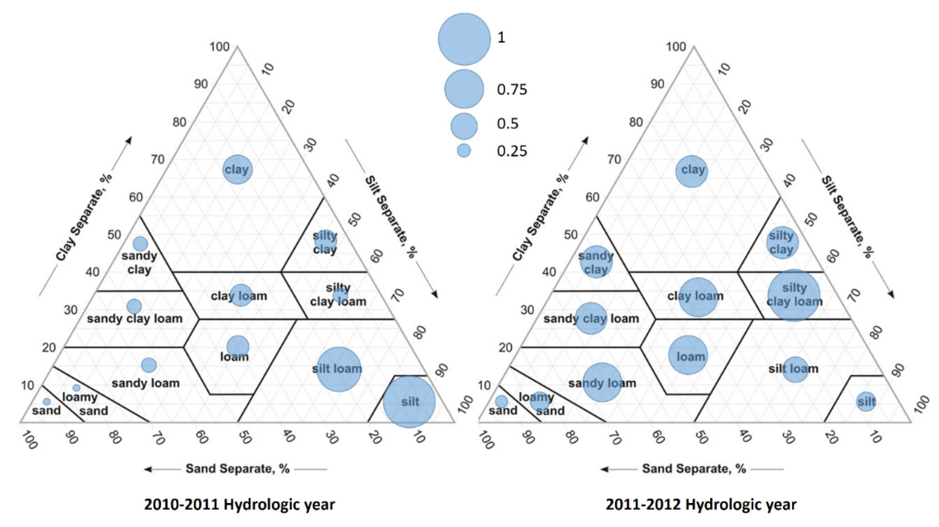
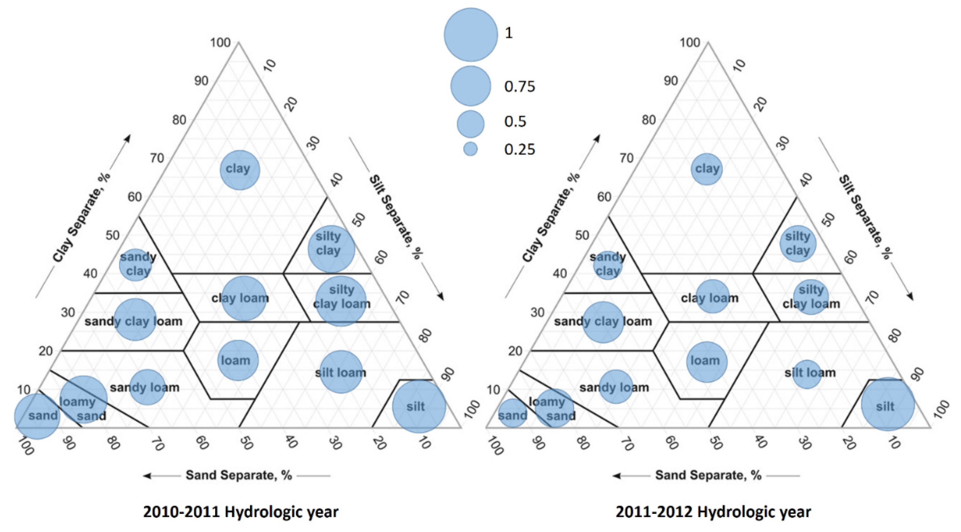
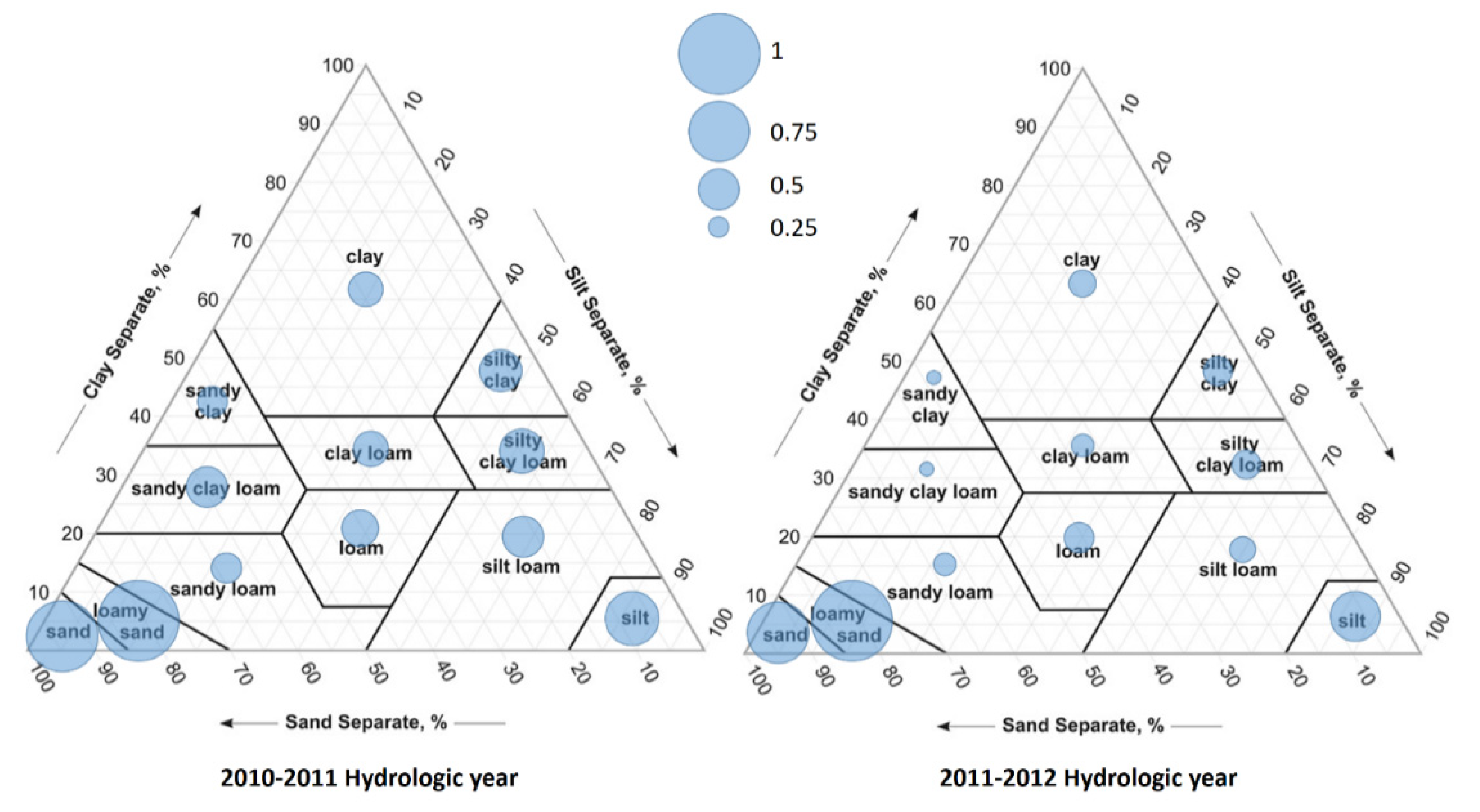
All metrics results were normalized between 0 and 1. Each soil texture within the USDA triangle has a circle which represents the scaled result (Figure 3, Figure 4, Figure 5, Figure 6 and Figure 7). A bigger circle (value of 1) indicates the highest value in that metric (i.e., a big circle in the FT cycles metric indicates a soil with several cycles within the year).
4.2.1. Freeze–Thaw Cycles (FTC)
Coarse soils such as sand are not as susceptible to freezing [12,42] as fine-textured soils such as loams, clays, and silt soils, which are more susceptible to freezing [56]. In fine-textured soil, if the freezing process is slow, the unfrozen moisture may move towards the freezing front, causing ice to accumulate in the upper layers [57]. When an FT process interacts with the soil, depending on the different soil textures, the soil structure might change. Fine-grained soil such as silt and clay are more vulnerable to FT cycles in their aggregate stability, while coarse-grained soils are more stable [3,58,59]. These behaviors are demonstrated in the model simulations (Table 2) where coarse soils (sand and loamy sand) have a lower number of FT cycles versus fine-textured soils such as clay and silt, which have higher fluctuations of FT cycles. This behavior is related to two processes: (i) the snowpack thickness (related to the air temperature), and (ii) the soil thermal conductivity.
The snowpack thickness and air temperature are important parts of the system, as they regulate system insulation capacity. A shallow snowpack in 2011–2012 coupled with high temperatures had less insulation capacity than a thicker snowpack and low temperature environment. It is clear that the 2011–2012 hydrologic year had higher temperatures in the winter and spring seasons than the 2010–2011 hydrologic year (Figure 1), which could explain the lower incidence of freeze–thaw cycles (e.g., warm environment, less ice; see normalized FTCs metric in Figure 3). Differences in the FT cycles between water years are apparent in the soil ice content for silt soil (1 cm depth). The 2010–2011 hydrologic year was more stable during winter, and it had more cycles when snowmelt and a shallow snow cover started to allow freeze–thaw processes in the soil during the spring season. In contrast, in the 2011–2012 hydrologic year, the ice content was quite unstable until the snowpack melted due to higher temperatures. For instance, fine-textured soils such as silt can have several freeze–thaw cycles, allowing water to infiltrate the soil below a thick snow cover. Under a shallower snow cover (2011–2012 hydrologic year), silt soil will have more FT cycles because of decreased insulation capability of the snow cover, which will produce more ice but also more thaw processes.
Higher water content can also enhance heat flow in soils, except for sand [60,61,62]. One possible explanation for this exception could be that the lower water content, particle contact (due to grain size and air content), and high permeability of sand do not allow many FT cycles, allowing for a roughly constant ice content. Silt soil has the lowest thermal conductivity among the four principal soils, but higher water content, better particle contact, low permeability, and higher water retention (due to pore size), which enhance heat flow.
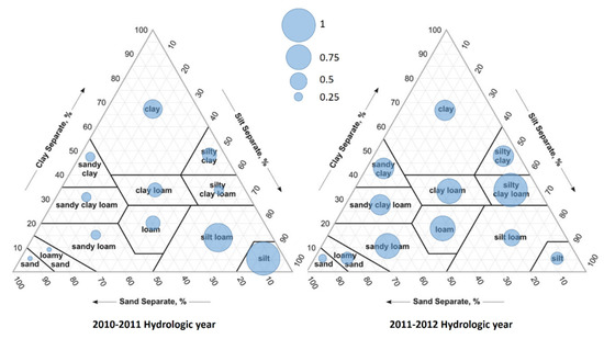
Figure 3.
Freeze–thaw cycles for 1 cm depth, 2010–2011 and 2011–2012 hydrologic years. Results were normalized ranging from 0 to 1; each circle represents the scaled result. A bigger circle indicates the highest value in the metric.
Figure 3.
Freeze–thaw cycles for 1 cm depth, 2010–2011 and 2011–2012 hydrologic years. Results were normalized ranging from 0 to 1; each circle represents the scaled result. A bigger circle indicates the highest value in the metric.
4.2.2. Maximum Ice Content
Coarse soils such as sand and loamy sand have less thermal conductivity because of the greater air content, lower soil water content, and less particle contact, causing a decrease in both convection and conduction. The particle–particle contact is an efficient heat transfer process [63] which make these soils thermal insulators, and as a result, less ice builds up within coarser soils.
Our results from the maximum ice content (example for all soils at 1 cm depth in Figure 4) metrics match the finer textured soil behavior, experiencing greater convection from the higher water content and greater conduction due to particle–particle contact. Fine-textured soils yield less ice due to efficient heat transfer processes, which causes more FT cycles to occur and increases ice production [64].
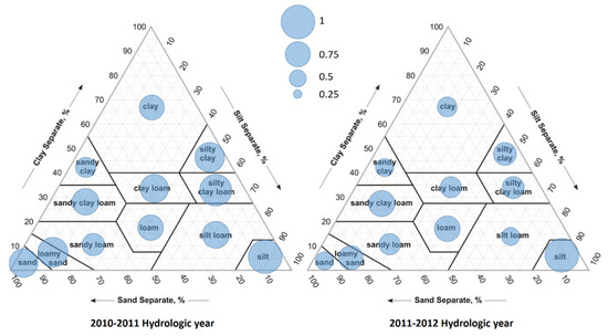
Figure 4.
Maximum ice content, 2010–2011 and 2011–2012 hydrologic years. Results were normalized ranging from 0 to 1; each circle represents the scaled result. A bigger circle indicates the highest value in the metric.
Figure 4.
Maximum ice content, 2010–2011 and 2011–2012 hydrologic years. Results were normalized ranging from 0 to 1; each circle represents the scaled result. A bigger circle indicates the highest value in the metric.
4.2.3. Days with Ice
Ambient air temperatures are a crucial factor in ice formation. Colder temperatures translate to more days with ice. In the first 2 cm within the soil profile, the snowpack is insulating the soil against warm air temperature; thus, a shallow snowpack will result in less ice formation and fewer days with ice, although the first 5 cm within the soil profile reflect how low air temperatures drive the soil ice content for sand, clay, and silt soils (Table 4). The 2010–2011 period had more snow and lower temperatures than the 2011–2012 period, which caused significantly more days with ice.
As a general comment, it seems that ice concentration in the upper layers may be due to water movement upwards due to pressure and temperature gradients. It may also be controlled by the differences in water content (silt and silty clay) and pore size (sand and loamy sand), i.e., bigger pores do not need higher pressure values to hold water.
For example, in study [20], the soil layer was a mix that contained a majority of sandy soil at the bottom and small layers of loamy soils at the top profile, and this soil had the fewest days with ice (e.g., 139 days at 1 cm depth in 2010–2017 period). These results are probably due to the saturated and residual water contents. Recalling the van Genuchten parameters, in [20], soils had the lowest saturated water content among the soils and zero residual water content. With less water available in the soil profile, there will likely be less freezing.
The days with ice metric (example for all soils at 1 cm depth in Figure 5) showed little difference between all 12 soils. This metric is related to two processes that are difficult to distinguish from one another within the model context: (i) fine-textured soils’ water content will increase the days with ice due to more water availability, and (ii) the diminished thermal conductivity of coarse soils can allow more ice formation and a slower or reduced thawing process.
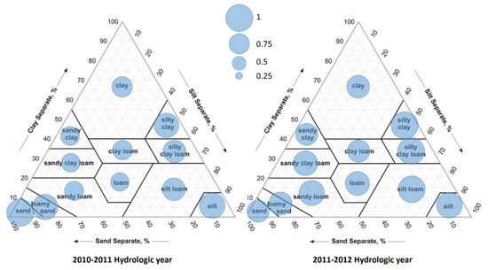
Figure 5.
Days with ice, 2010–2011 and 2011–2012 hydrologic years. Results were normalized ranging from 0 to 1; each circle represents the scaled result. A bigger circle indicates the highest value in the metric.
Figure 5.
Days with ice, 2010–2011 and 2011–2012 hydrologic years. Results were normalized ranging from 0 to 1; each circle represents the scaled result. A bigger circle indicates the highest value in the metric.

4.2.4. Temporal Ice Mass
The temporal ice mass is concentrated between 1 and 2 cm depth, and the depth of the largest temporal ice areas is around 8 cm. The coarse soils have the greatest temporal ice mass in the upper layers, which is caused by water suction from lower layers and the capacity to hold more water than the other soils (low initial soil water content). On the contrary, fine-textured soils have a diminished ability to suck water up due to less pore availability and higher initial soil water content (example at 1 cm depth in Figure 6).

Figure 6.
Temporal ice mass, 2010–2011 and 2011–2012 hydrologic years. Results were normalized ranging from 0 to 1; each circle represents the scaled result. A bigger circle indicates the highest value in the metric.
Figure 6.
Temporal ice mass, 2010–2011 and 2011–2012 hydrologic years. Results were normalized ranging from 0 to 1; each circle represents the scaled result. A bigger circle indicates the highest value in the metric.
4.2.5. Frost Depth
In general, the colder period (2010–2011) had deeper frost depth (Table 2 and Figure 7) than the warmer period (2011–2012). However, some exceptions were found. Sandy clay and clay froze to 14 cm depth, and they each had some of the lowest FT cycles in the 2010–2011 period, yet the same soils in the 2011–2012 period had a higher frost depth. One explanation is the shallow snowpack and thus a decreased insulation capacity. This result is noticeable in the FT cycles as well, where more cycles were found in the 2011–2012 hydrologic year.
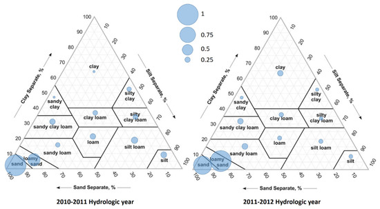
Figure 7.
Frost depth, 2010–2011 and 2011–2012 hydrologic years. Results were normalized ranging from 0 to 1; each circle represents the scaled result. A bigger circle indicates the highest value in the metric.
Figure 7.
Frost depth, 2010–2011 and 2011–2012 hydrologic years. Results were normalized ranging from 0 to 1; each circle represents the scaled result. A bigger circle indicates the highest value in the metric.

The thermal conductivity of coarse and fine-textured soils is different, and consequently, how the heat is transferred also varies. Hence, in a warmer environment, such as in 2011–2012, with a shallow snowpack, the temperature oscillation had a greater effect on these soils, and earlier snow accumulation will result in decreasing soil frost depth [65]. This delay can also lead to soil frost, which makes the soil less permeable for the spring snowmelt, as observed in 2011–2012, but thick snow cover appears to diminish this effect (e.g., [66,67]).
Frost depth can be explained then by (i) the soil permeability, (ii) the soil susceptibility to frost, (iii) the soil pore size, and (iv) the soil water content. Therefore, in fine-textured soils (clay and silt), it is more difficult for water to migrate towards the freezing front due to low permeability, which results in less ice formation [68]. Clay soils are better insulators than silt and sandy soils and more susceptible to forming ice layers due to their higher water content, which fills in the voids within the soil matrix [69]. Contrary to the behavior in clays, in coarse, sandy soils, water migrates towards the freezing front through the available void spaces [70]; thus, sand will likely have a greater frost depth than other soil textures. Moreover, because sand has more void spaces and lowest water content, it will have more air-filled porosity, and thus the sand will have lower values of thermal conductivity, reflecting the low thermal conductivity of air. The model did not account for these low values in the calculation. Instead, by using the ice and soil conductivities, which are higher than the thermal conductivity of air, the simulation erroneously showed a high thermal conductivity for sand.
In general terms, coarse soils such as sand and loamy sand have less thermal conductivity because of the greater air content, lower soil water content, and less particle contact, which causes a decrease in both convection and conduction. The particle–particle contact is an efficient heat transfer process [63], which make these soils thermal insulators, and as a result, less ice builds up within coarser soils.
4.3. Final Remarks
Thermal conductivity (λ) is enhanced by particle contact and the increasing water content in fine-textured soils, whereas in sandy and loamy sand coarse soils, low water content and high air content will reduce the thermal conductivity. Additionally, the thermal conductivity depends on the water phase evolution [71].
Two assumptions made by [72,73] were contrasted regarding soil thermal conductivity and soil texture. Ref. [72] mentioned that when the thermal conductivity and grain size decrease, this might be due to the presence of more particles within a soil; hence, more thermal resistance would exist among the particles, which seems to be contrary to our results. However, Ref. [74] mentioned that soils with low thermal conductivities might experience larger gradients in surface temperature, which agrees with our fine-textured results.
In contrast, Ref. [73] mentioned when the contact between soil particles increases, heat transfer is more efficient. Therefore, in fine-sized particle soils (silt and clay), the particle contact is more efficient than coarse soils. An example of this is the variability observed in finer textured soil within the freeze–thaw cycles. Ultimately, a primary driver is that the water content plays an important role in facilitating thermal exchange between soil particles, as our results also show.
The thickness of snowpack plays an important role as a soil insulator affecting soil temperature and energy fluxes into the subsurface [75,76,77], the temperature becoming another factor governing freeze–thaw process. A shallow snowpack allows more ice formation and less infiltration within the soil profile [78] and may increase the freeze–thaw cycles within the soil [79,80,81,82]. By contrast, a thicker snowpack insulates the soil, thereby maintaining a more moderate temperature and less building up of ice. In summary, thin snowpack during winter results in low soil temperatures, more FT cycles, and deeper and extensive soil freezing [83].
In vegetated areas with shallower snowpack, the uptake of water by roots has been shown to influence the soil water content. This is especially true in early spring, when the growing season begins after snowmelt. Plants can access root water and photosynthesize sooner due to a thinner snowpack and more incoming light. A shift in the snowfall (late snowpack) may affect the soil frost duration and depth [84,85], and soil freezing could lead to fine root mortality, affecting a tree’s development [77]. For instance, the simulated shallow snow cover in the 2011–2012 hydrologic year shows decreasing water content in silt and clay soil types. This behavior can be explained by (i) refreezing water from snow melt, (ii) increasing incoming radiation due to a thin snowpack, and (iii) root water uptake. The activity of plants beneath the snowpack can also disturb the frozen soil and allow snow melt [30]; however, this activity depends on the thickness of snowpack because plants need light to grow. The amount of available unfrozen water dictates plant uptake in late winter to early spring [86,87]. Because the 2011–2012 hydrologic year had more unfrozen water, it is possible that the decrease in soil water content is due to root water uptake stimulated by an increase in incoming light.
5. Conclusions
In two contrasting climatic years, we used a 1D numerical model (SCRM) coupling heat transport and water flow to synthesize the understanding of soil frost on 12 different soil textures at a snow-dominated site. Model simulation on these soils agreed with the knowledge about soil freezing–thawing processes. As we hypothesized, soil texture and soil hydraulic properties, such as water content, are the primary drivers that control the freeze–thaw process in soil. However, weather is another important factor affecting this process. Our results show that coarse soils are less conductive and subject to less convective processes (i.e., a good insulator) which combine to prevent ice formation within the soil profile. In contrast, the high particle–particle contact in fine-textured soil results in greater conductive heat transfer, and the high water content enhances thermal conductivity and convection processes. The metrics accurately described all these soil textures variations in the freeze–thaw process.
The freeze–thaw process is strongest in the period with the late snowpack according to the metrics described. Therefore, in the presence of a late snowfall and subzero air temperatures, the soil will freeze easily. Our results have shown that late snowfall will lead to more days with ice and a greater concentration and depth (especially in coarse textured soils). These results are due to the absence of the insulating capacity of snowpack.
Despite the inherent limitations of a synthetic simulation without real field data to compare, our study provides a methodological framework and metric references for future studies addressing and inferring freeze–thaw processes in soil in a snow-dominated forest site. This method is particularly important for understanding the implications of climate change in high mountain regions, where increasing temperatures will greatly affect rainfall patterns and the snowpack distribution [87,88,89].
Author Contributions
Conceptualization, F.B., T.P.A.F. and T.M.; methodology, F.B.; software, F.B.; formal analysis, F.B., T.P.A.F. and T.M.; investigation, F.B., T.P.A.F., T.M. and J.L.A.; writing—original draft preparation, F.B.; writing—review and editing, F.B., T.P.A.F., T.M. and J.L.A.; visualization, F.B. and T.P.A.F.; supervision, T.P.A.F., T.M. and J.L.A. All authors have read and agreed to the published version of the manuscript.
Funding
This research was funded by Chilean National Agency for Research and Development (Agencia Nacional de Investigación y Desarrollo de Chile, ANID) through project ANID/FONDAP/15130015, to the scholarship 2013-73140490, and to the doctoral scholarship ANID-PFCHA/Doctorado Nacional/2021-21210861 for the support of the lead author (F.B.).
Institutional Review Board Statement
Not applicable.
Informed Consent Statement
Not applicable.
Data Availability Statement
The data presented in this study are available on request from the corresponding author.
Acknowledgments
Thanks to Thijs Kelleners for allowing us to use his model, as well as for his assistance and suggestions.
Conflicts of Interest
The authors declare no conflict of interest.
References
- Fouli, Y.; Cade-Menun, B.J.; Cutforth, H.W. Freeze–Thaw cycles and soil water content effects on infiltration rate of three Saskatchewan soils. Can. J. Soil Sci. 2013, 93, 485–496. [Google Scholar] [CrossRef]
- Six, J.; Bossuyt, H.; Degryze, S.; Denef, K. A history of research on the link between (micro)aggregates, soil biota, and soil organic matter dynamics. Soil Tillage Res. 2004, 79, 7–31. [Google Scholar] [CrossRef]
- Kværnø, S.H.; Øygarden, L. The influence of freeze–thaw cycles and soil moisture on aggregate stability of three soils in Norway. CATENA 2006, 67, 175–182. [Google Scholar] [CrossRef]
- Zhang, L.; Ren, F.; Li, H.; Cheng, D.; Sun, B. The Influence Mechanism of Freeze-Thaw on Soil Erosion: A Review. Water 2021, 13, 1010. [Google Scholar] [CrossRef]
- Zaqout, T.; Andradóttir, H.; Arnalds, O. Infiltration capacity in urban areas undergoing frequent snow and freeze–thaw cycles: Implications on sustainable urban drainage systems. J. Hydrol. 2022, 607, 127495. [Google Scholar] [CrossRef]
- Qi, J.; Ma, W.; Song, C. Influence of freeze–thaw on engineering properties of a silty soil. Cold Reg. Sci. Technol. 2008, 53, 397–404. [Google Scholar] [CrossRef]
- Ouyang, W.; Shan, Y.; Hao, F.; Chen, S.; Pu, X.; Wang, M. The effect on soil nutrients resulting from land use transformations in a freeze-thaw agricultural ecosystem. Soil Tillage Res. 2013, 132, 30–38. [Google Scholar] [CrossRef]
- Guo, Z.R.; Jing, E.C.; Nie, Z.L.; Jiao, P.C.; Dong, H. Analysis on the characteristics of soil moisture transfer during freezing and thawing period. Adv. Water Sci. 2002, 13, 298–302. [Google Scholar]
- Niu, G.-Y.; Yang, Z.-L. Effects of Frozen Soil on Snowmelt Runoff and Soil Water Storage at a Continental Scale. J. Hydrometeorol. 2006, 7, 937–952. [Google Scholar] [CrossRef]
- Sartz, R.S. Test of Three Indirect Methods of Measuring depth of frost. Soil Sci. 1967, 104, 273–278. [Google Scholar] [CrossRef]
- Flerchinger, G.N.; Lehrsch, G.A.; McCool, D.K. Freezing and thawing processes. In Encyclopedia of Soils in the Environment; Hillel, D., Ed.; Elsevier: Oxford, UK, 2005; pp. 104–110. [Google Scholar]
- Bronfenbrener, L. The modelling of the freezing process in fine-grained porous media: Application to the frost heave estimation. Cold Reg. Sci. Technol. 2008, 56, 120–134. [Google Scholar] [CrossRef]
- Hansson, K.; Šimůnek, J.; Mizoguchi, M.; Lundin, L.C.; Genuchten, M.T.V. Water flow and heat transport in frozen soil. Vadose Zone J. 2004, 3, 693–704. [Google Scholar]
- Cox, P.M.; Betts, R.A.; Bunton, C.B.; Essery, R.L.H.; Rowntree, P.R.; Smith, J. The impact of new land surface physics on the GCM simulation of climate and climate sensitivity. Clim. Dyn. 1999, 15, 183–203. [Google Scholar] [CrossRef]
- Williams, P.J.; Burt, T.P. Measurement of Hydraulic Conductivity of Frozen Soils. Can. Geotech. J. 1974, 11, 647–650. [Google Scholar] [CrossRef]
- Hillel, D. Environmental Soil Physics: Fundamentals, Applications, and Environmental Considerations; Academic Press: Cambridge, MA, USA, 1998. [Google Scholar]
- Tokumoto, I.; Noborio, K.; Koga, K. Coupled water and heat flow in a grass field with aggregated Andisol during soil-freezing periods. Cold Reg. Sci. Technol. 2010, 62, 98–106. [Google Scholar] [CrossRef]
- Jansson, P.E.; Karlberg, L. Coupled Heat and Mass Transfer Model for Soil-Plant-Atmosphere Systems; Royal Institute of Technology: Stockholm, Sweden, 2010. [Google Scholar]
- Flerchinger, G.N. The Simultaneous Heat and Water (SHAW) Model: Technical Documentation; Technical Report for Northwest Watershed Research Center; USDA Agricultural Research Service: Washington, DC, USA, 2000.
- Kelleners, T.J.; Koonce, J.; Shillito, R.; Dijkema, J.; Berli, M.; Young, M.H.; Frank, J.M.; Massman, W. Numerical Modeling of Coupled Water Flow and Heat Transport in Soil and Snow. Soil Sci. Soc. Am. J. 2016, 80, 247–263. [Google Scholar] [CrossRef]
- Kelleners, T.J. Coupled water flow, heat transport, and solute transport in a seasonally frozen rangeland soil. Soil Sci. Soc. Am. J. 2020, 84, 399–413. [Google Scholar] [CrossRef]
- Kollet, S.J.; Maxwell, R.M. Capturing the influence of groundwater dynamics on land surface processes using an integrated, distributed watershed model. Water Resour. Res. 2008, 44, W02402. [Google Scholar] [CrossRef]
- He, H.; Dyck, M.F.; Si, B.C.; Zhang, T.; Lv, J.; Wang, J. Soil freezing–thawing characteristics and snowmelt infil-tration in Cryalfs of Alberta, Canada. Geoderma Reg. 2015, 5, 198–208. [Google Scholar] [CrossRef]
- Hardy, J.P.; Groffman, P.M.; Fitzhugh, R.D.; Henry, K.S.; Welman, A.T.; Demers, J.D.; Fahey, T.J.; Driscoll, C.T.; Tierney, G.L.; Nolan, S. Snow depth manipulation and its influence on soil frost and water dynamics in a northern hardwood forest. Biogeochemistry 2001, 56, 151–174. [Google Scholar] [CrossRef]
- Sharratt, B.; Benoit, G.; Daniel, J.; Staricka, J. Snow cover, frost depth, and soil water across a prairie pothole land-scape. Soil Sci. 1999, 164, 483–492. [Google Scholar] [CrossRef]
- Phillips, A.J.; Newlands, N.K. Spatial and temporal variability of soil freeze-thaw cycling across Southern Alberta, Canada. Agric. Sci. 2011, 2, 392. [Google Scholar] [CrossRef] [Green Version]
- Freppaz, M.; Williams, B.L.; Edwards, A.C.; Scalenghe, R.; Zanini, E. Simulating soil freeze/thaw cycles typical of winter alpine conditions: Implications for N and P availability. Appl. Soil Ecol. 2007, 35, 247–255. [Google Scholar] [CrossRef]
- Mellander, P.-E.; Löfvenius, M.O.; Laudon, H. Climate change impact on snow and soil temperature in boreal Scots pine stands. Clim. Change 2007, 85, 179–193. [Google Scholar] [CrossRef]
- Edwards, A.C.; Scalenghe, R.; Freppaz, M. Changes in the seasonal snow cover of alpine regions and its effect on soil processes: A review. Quat. Int. 2007, 162, 172–181. [Google Scholar] [CrossRef]
- Bayard, D.; Stähli, M.; Parriaux, A.; Flühler, H. The influence of seasonally frozen soil on the snowmelt runoff at two Alpine sites in southern Switzerland. J. Hydrol. 2005, 309, 66–84. [Google Scholar] [CrossRef]
- Solantie, R. Snow Depth on January 15th and March 15th in Finland 1919–98, and Its Implications for Soil Frost and Forest Ecology; Ilmatieteen Laitos: Helsinki, Finland, 2000.
- Xu, H.; Spitler, J.D. The relative importance of moisture transfer, soil freezing and snow cover on ground temperature predictions. Renew. Energy 2014, 72, 1–11. [Google Scholar] [CrossRef]
- Mellander, P.E.; Laudon, H.; Bishop, K. Modelling variability of snow depths and soil temperatures in Scots pine stands. Agric. For. Meteorol. 2005, 133, 109–118. [Google Scholar] [CrossRef]
- Oliva, M.; Ortiz, A.G.; Salvador, F.; Salvà, M.; Pereira, P.; Geraldes, M. Long-term soil temperature dynamics in the Sierra Nevada, Spain. Geoderma 2014, 235, 170–181. [Google Scholar] [CrossRef]
- Boike, J.; Roth, K.; Overduin, P. Thermal and hydrologic dynamics of the active layer at a continuous permafrost site (Taymyr Peninsula, Siberia). Water Resour. Res. 1998, 34, 355–363. [Google Scholar] [CrossRef]
- Stein, J.; Kane, D.L. Monitoring the unfrozen water content of soil and snow using time domain reflectometry. Water Resour. Res. 1983, 19, 1573–1584. [Google Scholar] [CrossRef]
- Motovilov, Y.G. Simulation of meltwater losses through infiltration into soil. Sov. Hydrol. 1979, 18, 217–221. [Google Scholar]
- Seyfried, M.S.; Grant, L.E.; Marks, D.; Winstral, A.; McNamara, J. Simulated soil water storage effects on streamflow generation in a mountainous snowmelt environment, Idaho, USA. Hydrol. Process. 2008, 23, 858–873. [Google Scholar] [CrossRef]
- Hirota, T.; Pomeroy, J.W.; Granger, R.J.; Maule, C.P. An extension of the force-restore method to estimating soil temperature at depth and evaluation for frozen soils under snow. J. Geophys. Res. Earth Surf. 2002, 107, ACL11. [Google Scholar] [CrossRef] [Green Version]
- Kang, M.; Lee, J. Evaluation of the freezing–thawing effect in sand–silt mixtures using elastic waves and electrical resistivity. Cold Reg. Sci. Technol. 2015, 113, 1–11. [Google Scholar] [CrossRef]
- Tian, H.; Wei, C.; Wei, H.; Zhou, J. Freezing and thawing characteristics of frozen soils: Bound water content and hysteresis phenomenon. Cold Reg. Sci. Technol. 2014, 103, 74–81. [Google Scholar] [CrossRef]
- Bronfenbrener, L.; Bronfenbrener, R.; Alafenish, A. A model of soils freezing with allowance for freezing zone. Chem. Eng. Process. Process Intensif. 2013, 73, 38–49. [Google Scholar] [CrossRef]
- Al-Houri, Z.; Barber, M.; Yonge, D.; Ullman, J.; Beutel, M. Impacts of frozen soils on the performance of infiltration treatment facilities. Cold Reg. Sci. Technol. 2009, 59, 51–57. [Google Scholar] [CrossRef]
- Rowlandson, T.L.; Berg, A.A.; Roy, A.; Kim, E.; Lara, R.P.; Powers, J.; Lewis, K.; Houser, P.; McDonald, K.; Toose, P.; et al. Capturing agricultural soil freeze/thaw state through remote sensing and ground observations: A soil freeze/thaw validation campaign. Remote Sens. Environ. 2018, 211, 59–70. [Google Scholar] [CrossRef]
- Saygili, A.; Dayan, M. Freeze-thaw behavior of lime stabilized clay reinforced with silica fume and synthetic fibers. Cold Reg. Sci. Technol. 2019, 161, 107–114. [Google Scholar] [CrossRef]
- Ogino, Y.; Matsuoka, N. Involutions resulting from annual freeze–thaw cycles: A laboratory simulation based on observations in northeastern Japan. Permafr. Periglac. Process. 2007, 18, 323–335. [Google Scholar] [CrossRef]
- Kelleners, T.; Verma, A. Modeling Carbon Dioxide Production and Transport in a Mixed-Grass Rangeland Soil. Vadose Zone J. 2012, 11, vzj2011.0205. [Google Scholar] [CrossRef]
- Celia, M.A.; Bouloutas, E.T.; Zarba, R.L. A general mass-conservative numerical solution for the unsaturated flow equation. Water Resour. Res. 1990, 26, 1483–1496. [Google Scholar] [CrossRef]
- Schaap, M.G.; Leij, F.J.; Genuchten, M.T.V. ROSETTA: A computer program for estimating soil hydraulic pa-rameters with hierarchical pedotransfer functions. J. Hydrol. 2001, 251, 163–176. [Google Scholar] [CrossRef]
- Gouttevin, I.; Krinner, G.; Ciais, P.; Polcher, J.; Legout, C. Multi-scale validation of a new soil freezing scheme for a land-surface model with physically-based hydrology. Cryosphere 2012, 6, 407–430. [Google Scholar] [CrossRef] [Green Version]
- Azmatch, T.F.; Sego, D.C.; Arenson, L.U.; Biggar, K.W. New ice lens initiation condition for frost heave in fi-ne-grained soils. Cold Reg. Sci. Technol. 2012, 82, 8–13. [Google Scholar] [CrossRef]
- Azmatch, T.F.; Sego, D.C.; Arenson, L.U.; Biggar, K.W. Using soil freezing characteristic curve to estimate the hydraulic conductivity function of partially frozen soils. Cold Reg. Sci. Technol. 2012, 83, 103–109. [Google Scholar] [CrossRef]
- Watanabe, K.; Wake, T. Hydraulic conductivity in frozen unsaturated soil. In Proceedings of the Ninth International Conference on Permafrost, Fairbanks, AK, USA, 29 June–3 July 2008; pp. 1927–1932. [Google Scholar]
- Spaans, E.J.; Baker, J.M. The soil freezing characteristic: Its measurement and similarity to the soil moisture char-acteristic. Soil Sci. Soc. Am. J. 1996, 60, 13–19. [Google Scholar] [CrossRef]
- Guymon, G.L.; Luthin, J.N. A coupled heat and moisture transport model for Arctic soils. Water Resour. Res. 1974, 10, 995–1001. [Google Scholar] [CrossRef]
- Wang, T.-L.; Yue, Z.-R.; Ma, C.; Wu, Z. An experimental study on the frost heave properties of coarse grained soils. Transp. Geotech. 2014, 1, 137–144. [Google Scholar] [CrossRef]
- Wang, T.-L.; Liu, Y.-J.; Yan, H.; Xu, L. An experimental study on the mechanical properties of silty soils under repeated freeze–thaw cycles. Cold Reg. Sci. Technol. 2015, 112, 51–65. [Google Scholar] [CrossRef]
- Guisheng, F.; Hongji, J.; Haiyan, L. Experimental study on main factors influencing water infiltration features of freezing and thawing soils. Trans. Chin. Soc. Agric. Eng. 1999, 15, 88–94. [Google Scholar]
- Bisal, F.; Nielsen, K.F. Effect of frost action on the size of soil aggregates. Soil Sci. 1967, 104, 268–272. [Google Scholar] [CrossRef]
- Rajaei, P.; Baladi, G.Y. Frost Depth: General Prediction Model. Transp. Res. Rec. J. Transp. Res. Board 2015, 2510, 74–80. [Google Scholar] [CrossRef]
- Smits, K.M.; Sakaki, T.; Limsuwat, A.; Illangasekare, T. Thermal Conductivity of Sands under Varying Moisture and Porosity in Drainage–Wetting Cycles. Vadose Zone J. 2010, 9, 172–180. [Google Scholar] [CrossRef]
- Chen, S.X. Thermal conductivity of sands. Heat Mass Transf. 2008, 44, 1241–1246. [Google Scholar] [CrossRef]
- Vargas, W.L.; McCarthy, J. Heat conduction in granular materials. AIChE J. 2001, 47, 1052–1059. [Google Scholar] [CrossRef]
- Meentemeyer, V.; Zippin, J. Soil moisture and texture controls of selected parameters of needle ice growth. Earth Surf. Process. Landf. 1981, 6, 113–125. [Google Scholar] [CrossRef]
- Iwata, Y.; Hayashi, M.; Hirota, T. Comparison of Snowmelt Infiltration under Different Soil-Freezing Conditions Influenced by Snow Cover. Vadose Zone J. 2008, 7, 79–86. [Google Scholar] [CrossRef]
- Henry, H.A.L. Climate change and soil freezing dynamics: Historical trends and projected changes. Clim. Change 2008, 87, 421–434. [Google Scholar] [CrossRef]
- IPCC. Intergovernmental Panel on Climate Change. Climate Change 2007; IPCC: Geneva, Switzerland, 2007.
- Andersland, O.B.; Ladanyi, B. An Introduction to Frozen Ground Engineering; John Wiley and Sons: Hoboken, NJ, USA, 2004. [Google Scholar]
- Penner, E. Ground Freezing and Frost Heaving (No. CBD-26); National Research Council of Canada: Ottawa, ON, Canada, 1962.
- Manohar, K.; Ramroop, K.; Yarbrough, D.W. Apparent Thermal Conductivity of Sand. In Proceedings of the Thermal Conductivity 27: Thermal Expansion 15: Joint Conferences, Knoxville, TN, USA, 26–29 October 2003; p. 461. [Google Scholar]
- Zhang, B.; Han, C.; Yu, X. A non-destructive method to measure the thermal properties of frozen soils during phase transition. J. Rock Mech. Geotech. Eng. 2015, 7, 155–162. [Google Scholar] [CrossRef] [Green Version]
- Tavman, I. Effective thermal conductivity of granular porous materials. Int. Commun. Heat Mass Transf. 1996, 23, 169–176. [Google Scholar] [CrossRef]
- Yun, T.S.; Santamarina, J.C. Fundamental study of thermal conduction in dry soils. Granul. Matter. 2008, 10, 197–207. [Google Scholar] [CrossRef]
- Abu-Hamdeh, N.H.; Reeder, R.C. Soil Thermal Conductivity Effects of Density, Moisture, Salt Concentration, and Organic Matter. Soil Sci. Soc. Am. J. 2000, 64, 1285–1290. [Google Scholar] [CrossRef]
- Cleavitt, N.L.; Fahey, T.J.; Groffman, P.M.; Hardy, J.P.; Henry, K.S.; Driscoll, C.T. Effects of soil freezing on fine roots in a northern hardwood forest. Can. J. For. Res. 2008, 38, 82–91. [Google Scholar] [CrossRef]
- Zhang, X.; Sun, S.F.; Xue, Y. Development and Testing of a Frozen Soil Parameterization for Cold Region Studies. J. Hydrometeorol. 2007, 8, 690–701. [Google Scholar] [CrossRef]
- Groffman, P.; Driscoll, C.T.; Fahey, T.J.; Hardy, J.P.; Fitzhugh, R.D.; Tierney, G.L. Colder soils in a warmer world: A snow manipulation study in a northern hardwood forest ecosystem. Biogeochemistry 2001, 56, 135–150. [Google Scholar] [CrossRef]
- Iwata, Y.; Hayashi, M.; Suzuki, S.; Hirota, T.; Hasegawa, S. Effects of snow cover on soil freezing, water movement, and snowmelt infiltration: A paired plot experiment. Water Resour. Res. 2010, 46, W09504. [Google Scholar] [CrossRef] [Green Version]
- Sinha, T.; Cherkauer, K.A. Impacts of future climate change on soil frost in the midwestern United States. J. Geophys. Res. Earth Surf. 2010, 115, D08105. [Google Scholar] [CrossRef] [Green Version]
- Decker, K.L.M.; Wang, D.; Waite, C.; Scherbatskoy, T. Snow Removal and Ambient Air Temperature Effects on Forest Soil Temperatures in Northern Vermont. Soil Sci. Soc. Am. J. 2003, 67, 1234–1242. [Google Scholar] [CrossRef] [Green Version]
- Herrmann, A.; Witter, E. Sources of C and N contributing to the flush in mineralization upon freeze–thaw cycles in soils. Soil Biol. Biochem. 2002, 34, 1495–1505. [Google Scholar] [CrossRef]
- Weih, M.; Karlsson, P.S. Low winter soil temperature affects summertime nutrient uptake capacity and growth rate of mountain birch seedlings in the subarctic, Swedish lapland. Arct. Antarct. Alp. Res. 2002, 34, 434–439. [Google Scholar] [CrossRef]
- Groffman, P.; Hardy, J.P.; Nolan, S.; Fitzhugh, R.D.; Driscoll, C.T.; Fahey, T.J. Snow depth, soil frost and nutrient loss in a northern hardwood forest. Hydrol. Process. 1999, 13, 2275–2286. [Google Scholar] [CrossRef]
- Shanley, J.B.; Chalmers, A. The effect of frozen soil on snowmelt runoff at Sleepers River, Vermont. Hydrol. Process. 1999, 13, 1843–1857. [Google Scholar] [CrossRef]
- Stadler, D.; Wunderli, H.; Auckenthaler, A.; Flühler, H.; Bründl, M. Measurement of frost-induced snowmelt runoff in a forest soil. Hydrol. Process. 1996, 10, 1293–1304. [Google Scholar] [CrossRef]
- Sutinen, R.; Hänninen, P.; Venäläinen, A. Effect of mild winter events on soil water content beneath snowpack. Cold Reg. Sci. Technol. 2008, 51, 56–67. [Google Scholar] [CrossRef]
- Vaganov, E.A.; Hughes, M.K.; Kirdyanov, A.V.; Schweingruber, F.H.; Silkin, P.P. Influence of snowfall and melt timing on tree growth in subarctic Eurasia. Nature 1999, 400, 149–151. [Google Scholar] [CrossRef]
- Harder, P.; Pomeroy, J.W.; Westbrook, C.J. Hydrological resilience of a Canadian Rockies headwaters basin subject to changing climate, extreme weather, and forest management. Hydrol. Process. 2015, 29, 3905–3924. [Google Scholar] [CrossRef]
- Nogués-Bravo, D.; Araújo, M.B.; Errea, M.P.; Martínez-Rica, J.P. Exposure of global mountain systems to climate warming during the 21st Century. Glob. Environ. Change 2007, 17, 420–428. [Google Scholar] [CrossRef]

Publisher’s Note: MDPI stays neutral with regard to jurisdictional claims in published maps and institutional affiliations. |
© 2022 by the authors. Licensee MDPI, Basel, Switzerland. This article is an open access article distributed under the terms and conditions of the Creative Commons Attribution (CC BY) license (https://creativecommons.org/licenses/by/4.0/).