Mathematical Functions to Model the Depth Distribution of Soil Organic Carbon in a Range of Soils from New South Wales, Australia under Different Land Uses

Abstract

The nature of depth distribution of soil organic carbon (SOC) was examined in 85 soils across New South Wales with the working hypothesis that the depth distribution of SOC is controlled by processes that vary with depth in the profile. Mathematical functions were fitted to 85 profiles of SOC with SOC values at depth intervals typically of 0–5, 5–10, 10–20, 20–30, 30–40, 40–50, 50–60, 60–70, 70–80, 80–90 and 90–100 cm. The functions fitted included exponential functions of the form SOC = A exp (Bz); SOC = A + B exp (Cz) as well as two phase exponential functions of the form SOC = A + B exp (Cz) + D exp (Ez). Other functions fitted included functions where the depth was a power exponent or an inverse term in a function. The universally best-fitting function was the exponential function SOC = A + B exp (Cz). When fitted, the most successful function was the two-phase exponential, but in several cases this function could not be fitted because of the large number of terms in the function. Semi-log plots of log values of the SOC against soil depth were also fitted to detect changes in the mathematical relationships between SOC and soil depth. These were hypothesized to represent changes in dominant soil processes at various depths. The success of the exponential function with an added constant, the two-phase exponential functions, and the demonstration of different phases within the semi-log plots confirmed our hypothesis that different processes were operating at different depths to control the depth distributions of SOC, there being a surface component, and deeper soil component. Several SOC profiles demonstrated specific features that are potentially important for the management of SOC profiles in soils. Woodland and to lesser extent pasture soils had a definite near surface zone within the SOC profile, indicating the addition of surface materials and high rates of fine root turnover. This zone was much less evident under cropping.

1. Introduction

Soil organic carbon (SOC) comprises 50 to 58% of soil organic matter (SOM) [1] and is an indicator of soil health and soil condition, with improvements in these typically being associated with increased amounts of SOC. Increasing SOC is also a method for removing carbon from the atmosphere to mitigate climate change and potentially to be a component in carbon trading schemes [2,3,4,5,6]. There are therefore two fundamental reasons for managing SOC: improving soil health and soil condition and the removal of CO₂ from the atmosphere.

Soil carbon accounting is usually focused on the surface soil horizons to 30 cm depth, and the International Panel on Climate Change (IPCC) has indicated that:

“For mineral soils, only the top 30 cm are considered, which typically has the highest concentration of carbon and the greatest response to changes in management and land use. In most soils, management effects on soil carbon at depth are minimal compared to changes that occur in the topsoil [7] and consequently most information on soil carbon responses to different management practices are limited to the upper soil horizons [0–30 cm depth].” [8].

Research to quantify and model SOC storage in these near surface layers is therefore extensive. However, predictions of SOC in deeper layers are less common. Estimation and prediction of SOC down the soil profile is increasingly important, as greenhouse gas (GHG) reductions and carbon trading schemes become more likely. Understanding the depth distribution of SOC across the landscape can assist in monitoring, managing and developing policy for SOC.

Depth distribution prediction and modelling is of particular use for a several reasons. Firstly, it can help identify the processes that lead to SOC sequestration, the depths at which these are most effective and can inform the selection and adoption of management practices that are most effective in sequestering carbon to different soil depths. Secondly, where data relating to the whole profile are unavailable, incomplete or unattainable (as in the case of broad-scale modelling), predictions can be made about SOC through the whole profile. Depth distribution functions have also been employed to express carbon density data as equivalent mass [9,10], which is now required for estimating SOC stocks in Australia [3]. Reliable depth functions may also be useful to reduce the cost of measuring or estimating SOC stores in soils which is considered one of the major limitations to the inclusion of SOC in trading schemes. Accurate, appropriate and widely applicable depth functions are therefore required across a range of soil types, environments and land-use types. The strength of such a modelling approach is that a simple integral can be applied across selected depths to mathematically estimate soil carbon distribution.

1.1. Mathematical Depth Functions

Depth functions have been investigated by a range of authors. For example, Russel and Moore [11], Kirkby [12], Dalal and Chan [13], Kempen et al. [14], Meersmans et al. [15] and Wiese et al. [16] determined that soil organic concentration declined with depth following simple exponential functions. Kirby [12] used a mass balance approach based on the inputs of organic materials from the soil surface and from plant roots along with the expected rates of decomposition and vertical mixing to determine depth distribution of SOC following an exponential distribution:

y_i = ∑_i a_i exp (−λ_i^½ z)

(1)

where y_i is the organic matter content of each fraction of organic matter [carbohydrates, lignin and amino acids] and z is the soil depth.

The actual depth distribution of SOC will be determined by the input and decomposition at each depth. Dalal and Chan [13] estimated SOC at a given soil depth using the following exponential function:

SOM_t = SOM₀ exp (−kt) + A/k (1−exp (−kt))

(2)

where SOM₀ and SOM_t are the SOM contents initially [t = 0], and at a given time, t, A [mass of SOM per unit area] is the rate at which organic matter is added to the soil at this depth increment and k [reciprocal of time] is the rate of loss of SOM or the rate of decomposition. The value of k will vary with the nature of the organic matter and the amount of soil carbon in each of the carbon pools or fractions. The values SOM₀, k and A will vary with depth.

At the soil surface, organic carbon input will include above ground plant litter as well as organic material from plant roots but for many soils over a wide range of depths, the root systems of plants will be the major input of organic carbon [17,18]. The rate of decomposition of SOM can be expected to decrease with depth because the soil environment is likely to have limited oxygen, less available water, lower concentrations of readily available nutrients (especially N) [19] and organic matter that is isolated from decomposers [20,21].

Minasny et al. [22] concluded that there are cases where the depth function of SOC may not follow a mathematical function, including soils under cultivation where the top layers have a uniform SOC content because of mixing by tillage [15,23] or where buried soils occur as is the case for paleosols [24]. Wong et al. [25] also observed the effect on the SOC depth distribution of a buried soil in a valley flat, where the SOC content bulged at a depth of 60 cm from 0.2% to 2.0%. The dark colour and nature of the soil indicated that this was a surface soil that had been buried by sediment from the actively eroding gully in the catchment above.

More recently, Hobley and Wilson [26] investigated the application of a separate exponential function to a set of data:

SOC[d] = SOC_Inf + (SOC₀−SOC_Inf) × exp (−d × k)

(3)

where SOC[d] is the mass concentration (%) of SOC as a function of depth below the soil surface, SOC_Inf is the mass concentration (%) of residual SOC in an “infinitely” deep soil, SOC₀ is the mass concentration (%) of SOC at the soil surface, d is the depth below the soil surface, k is the depletion constant [m⁻¹]. Equation (3) may be re-expressed using λ as the length scale of depletion in SOC concentration with depth [m], where λ = 1/k; this gives the equation:

SOC(d) = SOC_Inf + (SOC₀ − SOC_Inf) × exp (−d/λ)

(4)

They fitted the two equations [Equations (3) and (4)] separately to the data sets and so k and λ were determined independently from the data sets, even though they should be inversely related. A range of soil types were included in the data set, Luvisols, Lixisols, Solonetz, Vertisols and Nitosols based on WRB [27]. Soil samples were collected to 1.0 m depth with 6 to 12 samples per profile. In fitting these exponential models of SOC to soil depth, Hobley and Wilson [26] found adequate fits [based upon R² of fit and visual assessment of fitted function versus measured values] for 91 of the 100 profiles, mostly with a “good” to “excellent” model fit. The remaining nine soils had a much less reliable fit. This outcome is generally consistent with the conclusions from Minasny et al. [22], in that the depth distribution of SOC generally follows the root distribution which approximates an exponential decay function. Hobley and Wilson [26] investigated the most important factors that affected the value of the terms λ and k that determined the rate of decline of SOC with depth. They found that in general, land management factors were the most important, accounting for 52 to 67% of the variation in these variables, whether the land use was grazing, cropping or native vegetation. Other factors affecting these variables were temperature, amount of surface clay, ratio of surface to subsoil for silt, water holding capacity, nitrogen content and cation exchange capacity.

Traditionally, exponential functions have been used to describe the depth distribution of roots [28,29,30,31]. However, in an extensive international meta-analysis, Jobbagy and Jackson [32] found no direct relationship between the depth distribution of SOC and that of the root distribution of plants. Roots are generally distributed to more shallow depths than SOC, and SOC is typically distributed deeper in the soil than the proposed biomass source. Possible explanations given by Jobbagy and Jackson [32] included: (i) decreasing SOC turnover with depth, resulting in higher SOC accumulations per unit of C input in deep soil layers; (ii) increasing root turnover with depth, causing higher C inputs per unit of standing root biomass in deep soil layers; (iii) SOC translocation from upper to lower layers as dissolved organic carbon [33,34]; (iv) vertical mixing by soil organisms.

Given the complications often present in profile data of SOC, Bishop et al. [35] in [22] and Bonfetti et al. [10] proposed the use of equal-area quadratic smoothing splines to fit depth functions to SOC depth data instead of a single exponential function or other relatively simple mathematical function. While this process enables virtually any depth distribution to be fitted by a mathematical function and is good for data fitting and data prediction, this process does have the disadvantage of being largely a data fitting exercise, but does not account for any of the processes that control the depth distribution of SOC in the profile. Where spodic horizons occur in the subsoil, the depth distribution can show a peak type depth function [22], where the illuviated SOC accumulates in the spodic horizon below the soil surface [27].

A range of other approaches and functions have been employed to model and predict the distribution of SOC with depth. A list of the possible functions is shown in

Table 1. Predictive depth functions applied to the soil organic profiles from New South Wales. Equation numbers relate to descriptions in the text.

Equation	Name	Mathematical Form
5	Exponential	SOC = B exp (Cz)
6	Exponential	SOC = A + B exp (Cz)
7	Two phase exponential	SOC = B exp (Cz) + D exp (Ez)
8	Two phase exponential	SOC = A + B exp (Cz) + D exp (Ez)
9	Power function	SOC = BzC
10	Power function	SOC = A + BzC
11	Inverse	SOC = B/(1 + BCz)
12	Inverse	SOC = A + B/(1 + BCz)

. One of the most commonly used [36,37,38,39] is the negative exponential functions of the form:

Y = B exp (Cz)

(5)

and:

Y = A + B exp (Cz)

(6)

where Y is the SOC concentration in g/100 g of soil and z is the soil depth in cm, and A, B and C are model parameters to be estimated.

A justification for such an approach is that exponential decay functions can be readily explained by invoking common ecological and soil processes. For example, Cook and Kelliher [40] and Fang and Moncrieff [41] observed exponential decline in root mass and microbial biomass with depth in soil.

More complex exponential models have been applied with two distinct components (a ‘fast’ and a ‘slow’ component) to account for the step-wise but additive change rate processes that are often observed through space and time (e.g., [42,43]). These take the general form [with or without a defined SOC_∞ factor]:

Y = B exp (Cz) + D exp (Ez)

(7)

and:

Y = A + B exp (Cz) + D exp (Ez)

(8)

Such an approach was applied successfully by Meersmans et al. [15] to model depth distribution of SOC across a range of land-uses in Belgium. However, this approach implies that simple single exponential functions are insufficient to account for the complexity of the processes taking place. In the case of SOC distribution, single exponential functions tend to be applied and fit well to soils with a ‘symmetrical’ constant decay rate curve form in soils with limited surface SOC accumulation. However, more complex models might be required where large accumulations of SOC are concentrated in the near surface layers and depth distribution has a strong depth asymmetry [10].

Other forms of function that have been applied to SOC depth distribution include a range of power functions of the form:

Y = Bz^C

(9)

and:

Y = A + Bz^C

(10)

Such functions can often be fitted very precisely to specific data sets [22]. However, these functions have typically been generated and fitted to datasets that represent either a limited range of soil types and environments, a limited range of land-uses or both. Their specific and empirical nature also limits their application beyond the data from which they are derived. Many such functions are also often limited by the lack of a definite ‘intercept’ but rather asymptote to very large Y values at low values of z. This behaviour seems intuitively flawed with respect to SOC distribution. It is also difficult to derive a rationale or theoretical explanation for the reason the SOC depth distribution should fit a power function. However, as power functions can frequently describe natural systems, it was considered potentially useful to include this set of functions in the range of models tested.

The use of inverse functions to describe physical processes where there is a decay or diminished value with time or depth has also been used in the past. Therefore, we also investigated the use of this function to predict depth functions of SOC.

Y = B/(1 + BCz)

(11)

and:

Y = A + B/(1 + BCz)

(12)

More recently, Minasny et al. [44] have employed spline curve fitting to non-continuous data to estimate SOC down the profile, where, for example, soil profiles rather than depth intervals have been sampled and hence continuous data are not available. This approach has been successfully applied to mapping exercises, but the broad application of the functions derived has not yet been demonstrated. The spline function approach also has no theoretical or conceptual basis for its application and is largely a data fitting exercise.

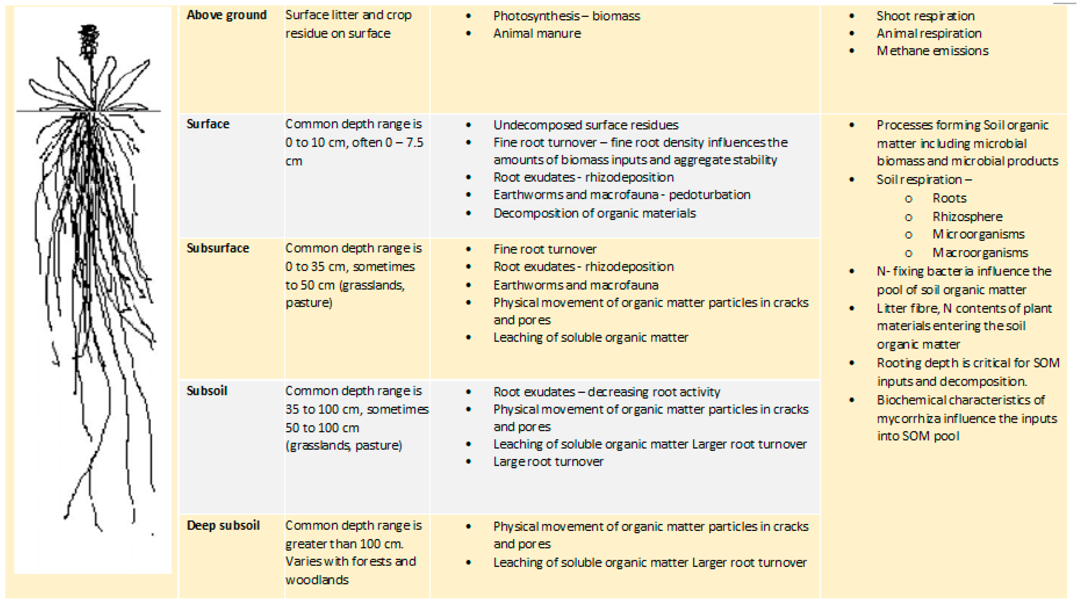
1.2. Conceptual Basis for Different Depth Zones in the Depth Distribution of Soil Organic Carbon

Soil organic carbon concentration in Australian soils is typically largest in the near surface soil layers declining rapidly with depth in the soil profile. The distribution of SOC is significantly affected by land-use and changes in SOC content of soils resulting from land-use change tend to occur preferentially in these surface layers [45]. Therefore, the net result of land-use change is to modify the depth distribution of soil down the profile. However, the distribution pattern of SOC with depth differs considerably between soil types and land-uses and understanding the depth distribution of SOC requires consideration of a number of interacting processes.

The depth distribution can be attributed to several sources [17] including: above ground plant litter input at the surface; below ground plant litter input within the soil, root litter, rhizodeposition, which includes organic carbon released by living roots into the rhizosphere [46,47], organic carbon from animals, organic carbon inputs from microbial sources including fungal and bacterial sources and translocation of organic carbon inputs by diffusion of water soluble organic carbon, mixing by soil fauna and land management effects especially tillage. The amount and type of additions of organic carbon will depend on the biomass production of plants and root distributions, climate, soil type and land management practices.

Once organic materials are added to soils, they are subjected to decomposition and the rate of decomposition will vary depending on its source and the local environment, including soil depth [19,48,49].

A conceptual model of SOC dynamics proposed by Eyles et al. [50] identifies several different zones in the soil where SOC cycling is governed by different interacting above-ground and below-ground processes. Adapting the model from Eyles et al. [50], we propose that the following zones can potentially be identified in soil where there are differences in the SOC dynamics [see Figure 1]:

1.2.1. Phase A—Surface Soil

Close to the surface, SOC is largely added by surface accumulation of biomass from plant litter at or near the surface [52]. Undecomposed residue from plants and some animal products are added to the soil surface, which contribute to the formation of humus for soil organic matter [53]. In the case of cropping, the depth of this layer can be affected by cultivation, with tillage tending to produce a uniform SOC distribution with depth through the disturbed layer [15,54,55,56,57,58]. However, this does depend on the depth of tillage and the implements used, as shallow cultivation (<10 cm) under cropping may not result in a surface layer with a uniform SOC [56,59]. Soil fauna such as can earthworms and ants can translocate some organic carbon from the surface [60,61,62], but this is typically limited to about 30 cm. Turnover of organic matter in this zone can be expected to take in the order of years or less.

1.2.2. Phase B—Subsurface, Upper Subsoil

At moderate depth, where organic carbon is added to the soil largely from root activity, especially fine or lateral root activity, exudates or rhizodeposition [17,18,63,64,65,66]. It also includes a minor component of translocation of surface organic materials as soluble carbon or particulate organic carbon. Microbial activity, especially fungal growth can also add organic carbon to this layer. Cereals and grasses are especially effective in adding soil organic matter with these processes because of their fibrous root systems that have a large volume of fine roots [17,66]. Turnover of organic matter in this zone can be expected to be in the order of 10 s of years [67].

1.2.3. Phase C—Subsoil

Deeper in the soil, where the root activity has diminished, especially fine root activity, root density is much reduced and influences a much smaller volume of soil. In this zone, there is less rhizodeposition and a much slower turnover of fine roots. Coarse soil structure can influence the root architecture and the flow patterns in the soil and so the distribution of dissolved SOM. As a consequence, some SOC can be concentrated in biopores, preferential flow paths or on the outside of peds and in cracks between peds as preferred paths for root growth [47,58,68]. As a consequence, the spatial variability in SOC is higher in subsoils than in the surface soils [58]. Translocation by water soluble SOC and POC from the surface can occur in this zone. Decomposition rates are slower in the deeper subsoil because of reduced oxygen, nutrients and moisture availability [19] and the relative isolation of organic matter from decomposer organisms [20,21]. SOC is often much older in this zone [67] and turnover can be expected to take 100 s of years.

1.2.4. Phase D—Deep Subsoil

This zone is largely below the level of root activity and the concentration of SOC falls substantially as there are few additions of fresh organic carbon. At this depth, much of the SOC is in the residual or passive pool and turnover can be expected in the 1000’s of years.

The distribution of soil SOC with depth can be complicated by the input of organic carbon from above ground plant litter and root growth from previous plant growth cycles. The organic carbon in the soil can be decomposing organic materials from plants that were grown in the soil from previous years. The depth distributions of soil organic matter may therefore represent successions of inputs and decomposition cycles of organic materials. Microorganisms can also affect the decomposition rates of organic materials firstly by being the agents that decompose the organic matter, but they can also control the types of end products that are produced. Some microorganisms can produce some of the more resistant organic compounds such as aliphatic carbon compounds, chitin and glomalin [17].

The depth distribution of SOC as determined at one point in time will reflect the net result of a range of processes, several of which can be operating at different rates and at different stages. This has implications for the mathematical description of the depth distributions of SOC, as discussed below.

1.3. Aims

Here, we sought to evaluate the suitability of a range of potential SOC distribution functions across a range of soils and land-uses in NSW, Australia. We first considered some of the factors influencing the distribution of SOC with depth, evaluated some observed distributions and then tested the applicability of four main approaches to depth distribution modelling, namely; negative exponential, power, reciprocal and two-phase negative exponential. For each function we tested an approach with and without a defined “intercept”, giving eight functions in all. We applied these potential functions to 85 soil profiles sourced from a range of sites, soil types and land-uses across NSW. Profiles of SOC are also investigated in detail based on the hypothesis that in any one soil profile, several processes are likely to be determining the depth distribution of SOC. Our objective was to attempt to fit different mathematical functions to the SOC depth profiles to gain insights into the characteristics and possible biophysical features of the SOC profiles.

2. Methods

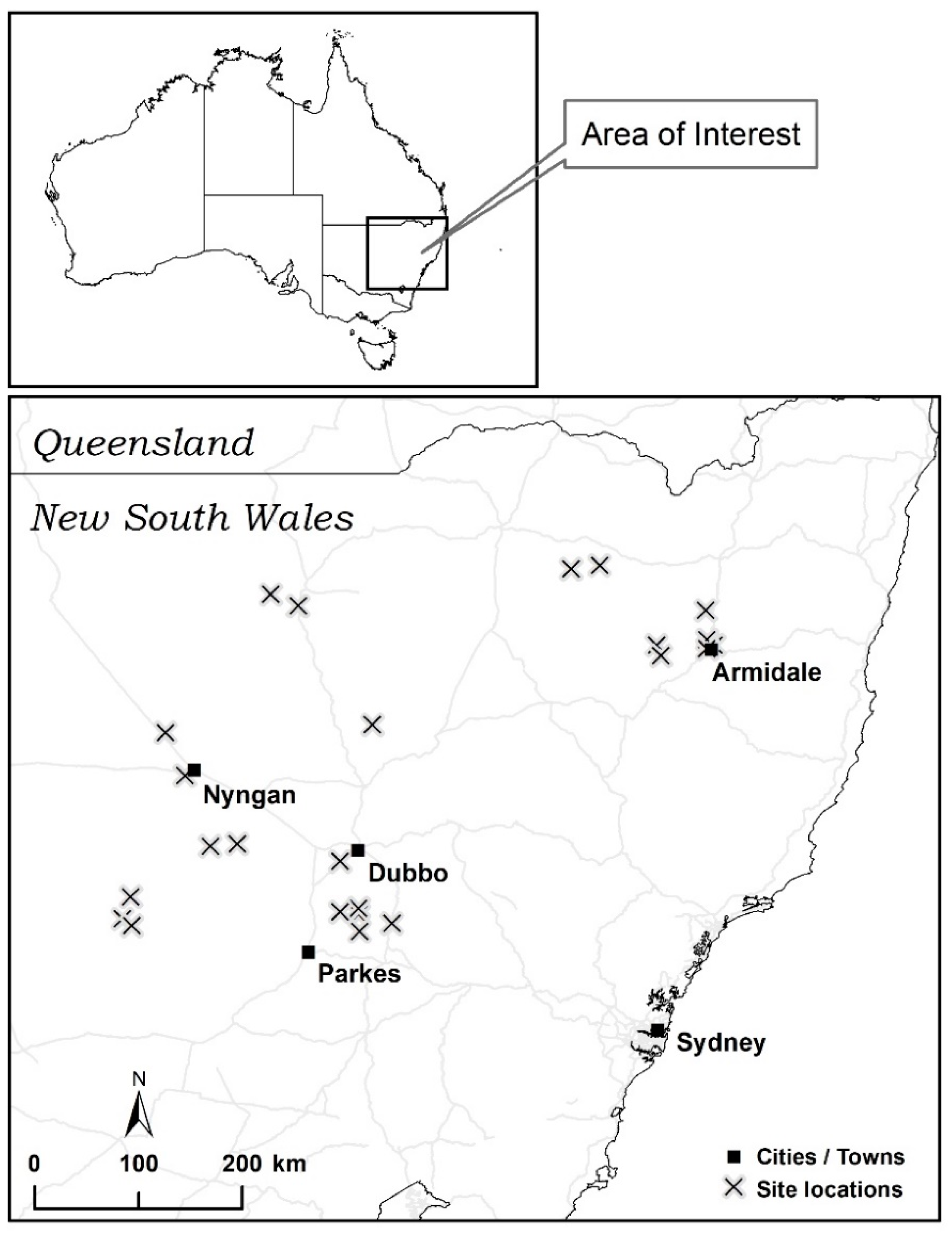
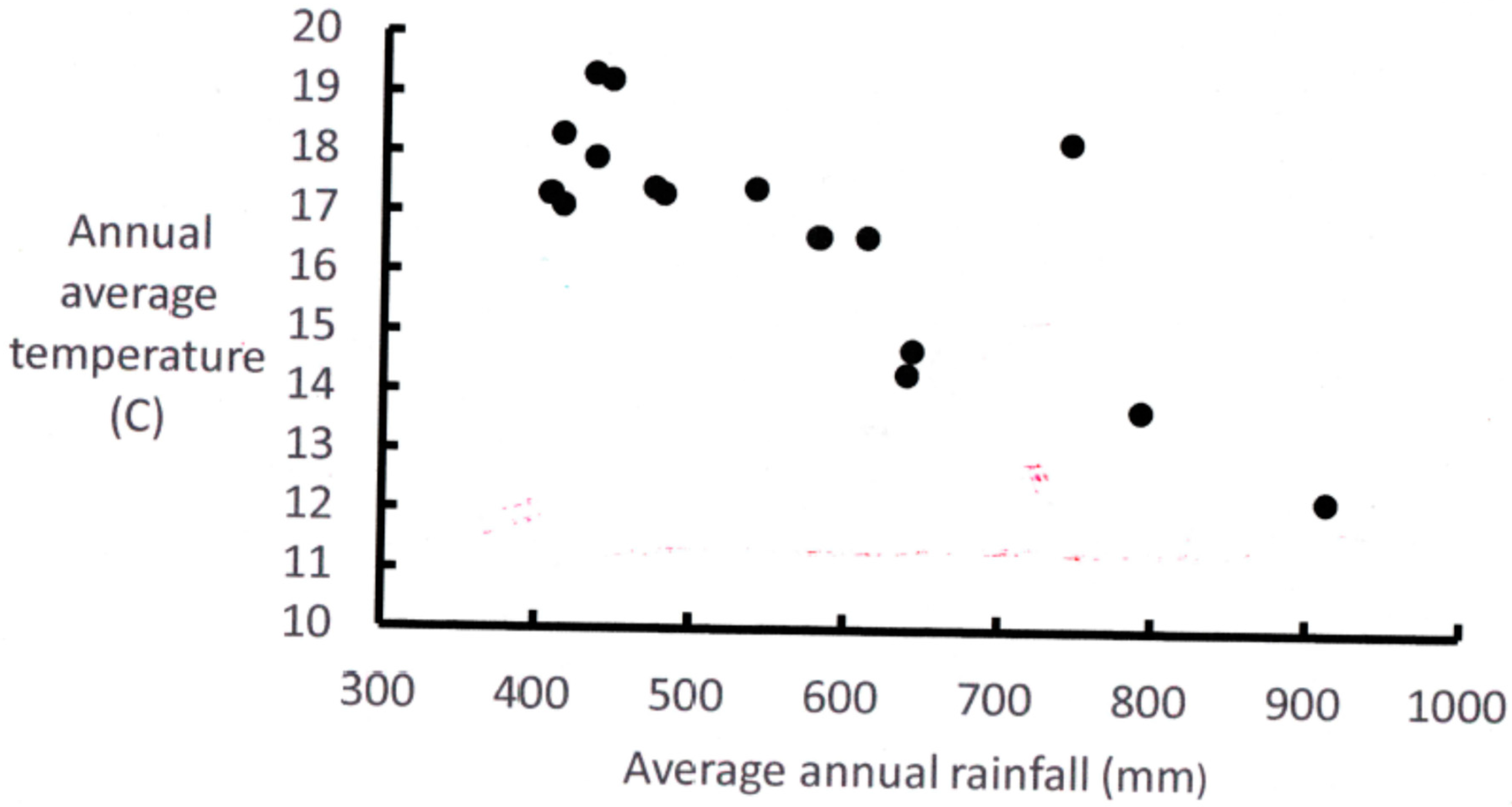
2.1. Site Descriptions

A total of 85 soil profiles were examined, sourced from a range of locations, soil types and land-uses across NSW. Summary data relating to each of these sites and profiles is provided in

Table 2. Site details. GO is Australian Greenhouse Office set of profiles. LR is Little River set of profiles. MAR is mean annual rainfall. MAT is mean annual temperature.

Parent Material	Location	Grid Reference	Soil Type	Land Use	Sampling Depth [cm]	MAR [mm]	MAT C	Site Number
New England Tablelands
Bingara Metasediments BM	Yeral/pinetrees	−29.79, 150.70	Red Chromosol	Woodland	100	745	18.2	BM1
	Yeral/pinetrees	−29.79, 150.70	Red Chromosol	Pasture	100	745	18.2	BM1
	Yeral/pinetrees	−29.79, 150.70	Red Chromosol	Cropping	100	745	18.2	BM1
	Dingwall	−29.82, 150.45	Red Chromosol	Woodland	100	745	18.2	BM2
	Dingwall	−29.82, 150.45	Red Chromosol	Pasture	100	745	18.2	BM2
	Dingwall	−29.82, 150.45	Red Chromosol	Cropping	100	745	18.2	BM2
Rockvale Metasediments RM	Rockvale	−30.48, 151.69	Yellow Chromosol	Woodland	80	792	13.7	RM-W1 to W5
	Rockvale	−30.48, 151.69	Yellow Chromosol	Pasture	80	792	13.7	RM-P1 to P5
Tulimba Metasediments TM	Tullimba	−30.48, 151.19	Yellow Chromosol	Woodland	70	643	14.7	TM1
	Tullimba	−30.48, 151.19	Yellow Chromosol	Pasture	70	643	14.7	TM2
Guyra Basalt Tertiary basalt GB	Kirby	−30.43, 151.63	Dermosol	Woodland	85	792	13.7	GB1
	Kirby	−30.43, 151.63	Dermosol	Native pasture	85	792	13.7	GB1
	Glendon	−30.18, 151.62	Black Ferrosol	Woodland	95	913	12.2	GB2
	Glendon	−30.18, 151.62	Black Ferrosol	Native pasture	95	913	12.2	GB2
Newby Park basalt Tertiary basalt NPB	Armidale	−30.51, 151.63	Brown Dermosol	Woodland	100	792	13.7	NPB-W1 to W5
	Armidale	−30.51, 151.63	Brown Dermosol	Native pasture	100	792	13.7	NPB-P1 to P5
Camerons Granite CG	Kingstown	−30.57, 151.23	Yellow Chromosol	Woodland	100	640	14.3	CG1
	Kingstown	−30.57, 151.23	Yellow Chromosol	Pasture	100	640	14.3	CG1
Central West NSW, Australian Greenhouse Office [AGO]—land clearing
Granite colluvium	Tallebung, NW of Condobolin	−32.91, 146.65	Red Kandodsol	Woodland	100	407	17.3	AGO1
Granite colluvium	Tallebung, NW of Condobolin	−32.91, 146.65	Red Kandosol	Cropping [cleared 3 years]	100	407	17.3	AGO2
Granite colluvium	Tallebung, NW of Condobolin	−32.85, 146.57	Red Kandosol	Woodland	100	408	17.3	AGO3
Granite colluvium	Tallebung, NW of Condobolin	−32.91, 146.65	Red Kandosol	Cropping [cleared 3 years]	100	408	17.3	AGO4
Granite colluvium	Tallebung, NW of Condobolin	−32.66, 146.64	Red Kandosol	Woodland	100	416	17.1	AGO5
Granite colluvium	Tallebung, NW of Condobolin	−32.66, 146.64	Red Kandosol	Pasture	100	416	17.1	AGO6
Granite colluvium	Tallebung, NW of Condobolin	−32.66, 146.64	Red Kandosol	Cropping [cleared > 25 years]	100	416	17.1	AGO7
Central West NSW, Australian Greenhouse Office [AGO]—land clearing [Murphy et al. 2003]
Girilambone Beds	Tottenham	−32.22; 147.33	Red Kandosol	Woodland	100	475 mm	17.4	AGO8
Girilambone Beds	Tottenham	−32.22; 147.33	Red Kandosol	Cropping [cleared > 25 years]	100	475 mm	17.4	AGO9
Quaternary Alluvium	Dandaloo/ Narromine	−32.20; 147.56	Grey Vertosol	Woodland	100	481 mm	17.3	AGO10
Quaternary Alluvium	Dandaloo/ Narromine	−32.20; 147.56	Grey Vertosol	Cropping [cleared 20 years]	100	481 mm	17.3	AGO11
Girilambone Beds	Girilambone	−31.24; 146.94	Red Kandosol	Woodland	100	415 mm	18.3	AGO12
Girilambone Beds	Girilambone	−31.24; 146.94	Red Kandosol	Cropping [cleared 9 years]	100	415 mm	18.3	AGO13
Girilambone Beds	Nyngan	−31.61; 147.11	Red Kandosol	Woodland	100	437 mm	17.9	AGO14
Girilambone Beds	Nyngan	−31.61; 147.11	Red Kandosol	Cropping [cleared 8 years]	100	437	17.9	AGO15
Quaternary Alluvium	Coonamble	−31.17; 148.73	Grey Vertosol	Woodland	100	541	17.4	AGO16
Quaternary Alluvium	Coonamble	−31.17; 148.73	Grey Vertosol	Cropping [cleared > 25 years]	100	541	17.4	AGO17
Quaternary Alluvium	Walgett	−30.14; 148.09	Grey Vertosol	Woodland	100	447	19.2	AGO18
Quaternary Alluvium	Walgett	−30.14; 148.09	Grey Vertosol	Cropping [cleared 6 years]	100	447	19.2	AGO19
Quaternary Alluvium	Walgett	−30.14; 148.09	Grey Vertosol	Cropping [cleared > 25 years]	100	447	19.2	AGO22
Quaternary Alluvium	Walgett	−30.04; 147.85	Grey Vertosol	Cropping [cleared 6 years]	100	436	19.3 °C	AGO20
Quaternary Alluvium	Walgett	−30.04; 147.85	Grey Vertosol	Cropping [cleared 6 years]	100	436	19.3	AGO21
Central West NSW, Little River Hydrological Study [LR] [McKenzie 2002]
Cowra Trough Metasediments	Yeoval 1; Arthurville	−32.35; 148.45	Brown Sodosol	Pasture-lucerne	140	583	16.6	LR1
	Yeoval 7; Cumnock	−32.89; 148.90	Red Dermosol	Cropping	140	613	16.6	LR7
Yeoval Granite	Yeoval 2; Yeoval	−32.81; 148.61	Red Kandosol	Pasture-lucerne	140	581	16.6	LR2
	Yeoval 3; Yeoval	−32.76; 148.61	Red Chromosol	Pasture	120	581	16.6	LR3
	Yeoval 4; Yeoval	−32.79; 148.45	Rudosol/Tenosol	Pasture	37	581	16.6	LR4
	Yeoval 5; Yeoval	−32.79; 148.45	Yellow Chromosol	Pasture	130	581	16.6	LR5
Dulladerry Rhyolite	Yeoval 6; Cumnock	−32.96; 148.62	Yellow Chromosol	Cropping	130	613	16.6	LR6

and their locations in Figure 2. The range of climates is indicated in Figure 3, showing the temperatures and average annual rainfall. The range of climates covers those commonly occurring in the inland tablelands, slopes and plains of south-eastern Australia [69]. The profiles of SOC were chosen such that the SOC data extended often to a depth of 100 cm, but least to 70 cm, and with at least eight measurements within the profile [see Table 2]. Further criteria were that the topsoil had data for at least the depth intervals of 0 to 5 cm, 5 to 10 cm, 10 to 20 cm and 20 to 30 cm. Soils in the study included Red and Yellow Chromosols, Red Kandosols, Dermosols, Ferrosols and Grey Vertosols [70]. The equivalent soils in the World Reference Base are Red and Yellow Luvisols, Red and Yellow Lixisols, Nitosols, Ferralsols and Grey Vertisols [27].

The SOC data were collected during the progress of several carbon projects. SOC profiles from the New England Tablelands in Northern NSW were analysed and this study was part of the Australian Soil Carbon Research Project (SCaRP) [71]. This study included sites on granite, basalt and metasediments and across a range of land uses including woodlands, pasture and cropping [45,72,73,74,75]. Further SOC profiles were taken from a survey of the impact of land clearing on SOC in central NSW [76] and involved measurements on paired sites of cleared and uncleared native vegetation on Red Chromosols, Red Kandosols and Grey Vertosols on the central west slopes and plains of New South Wales. A final set of SOC profiles was taken from a study in the Little River Catchment of NSW [77], which is on the central west slopes of New South Wales and included pasture and cropping sites.

The SOC data were collected using a standard methodology of extracting soil cores to the specified depth, which were then sub-divided into selected depth intervals [78,79,80]. The wet weight of the soil in the depth interval was recorded and then a sample taken so that the field moisture content at the time of sampling could be determined. Using the diameter of the core, the depth interval and the wet weight of soil and the field moisture content of the soil, the bulk density based on oven dry soil was calculated for each depth interval. The SOC content was determined using a Leco furnace. The methodology is provided in detail in Murphy et al. [76]. For the Australian Greenhouse Office Project [76], the diameter of the core was 150 mm. For the Little River hydrological study, the diameter of the core was 75 mm [77]. The collection of samples and analysis for the New England samples is described in Wilson et al. [45,73]. Typically, 5–10 replicate soil cores per site were averaged at each depth interval and used in these analyses.

2.2. Statistical Analysis

2.2.1. Fitting Curves to Depth Distributions

Here, we attempted to fit eight potential mathematical functions as shown in Table 1. The curve fitting process was undertaken using the Genstat Statistical package [81] and the specialist curve fitting software TableCurve 2D [82]. For each SOC profile the goodness of fit of the models was judged using the coefficient of determination [adjusted R²], the Standard Error of the Estimate (SEE), and the Akaike Information Criterion (AIC). The adjusted R² indicates the proportion of the regression mean square of the dependent variable that is attributed to the predictor variable[s]. The SEE statistic is simply the square root of the Error Mean Square term from the regression, and hence, it is an unbiased estimate of the true variance about the regression [83]. The AIC statistic is a function of the residual deviance penalised by adding twice the estimated parameters in the fitted model [84]. This penalty serves to discourage against the overfitting of models. For each SOC profile, the aim was to give preference to models with low levels of relative lack of fit (lower values for SEE and AIC are preferred), and higher levels of relative adequacy of fit (higher values of adjusted R² are preferred).

2.2.2. Evaluating SOC Distributions within Depth Segments Using Semi-Log Plots

Because many of the depth distributions still showed poor fitting to some portion of the depth range, an investigatory approach using semi-log plots was considered potentially useful. If the relationship between SOC and depth can be described by a simple exponential relationship, then a plot of log_e (SOC) with depth (z) should result in a straight line such that:

log_e(SOC) = mz + b

(13)

By back-transformation of the coefficient b from Equation [13], namely G = exp[b], the simple exponential function of Equation [5] can be derived, namely SOC = G * exp(mz), where G estimates the value of SOC at the soil surface where depth (z) = 0.

Conceptually, a semi-log plot of the SOC distribution with depth can be used to identify the zones in which different processes dominate the SOC distribution with depth. As discussed in Section 3.2, it is hypothesized that there are potentially three to four distinct zones at different depths within the soil where different processes control the depth distribution of SOC. The zones were selected where there was a straight line segment in the log_e(SOC) v depth plots. The depth and occurrence of these zones in particular soil can be expected to vary with the climate soil type and management history.

3. Results

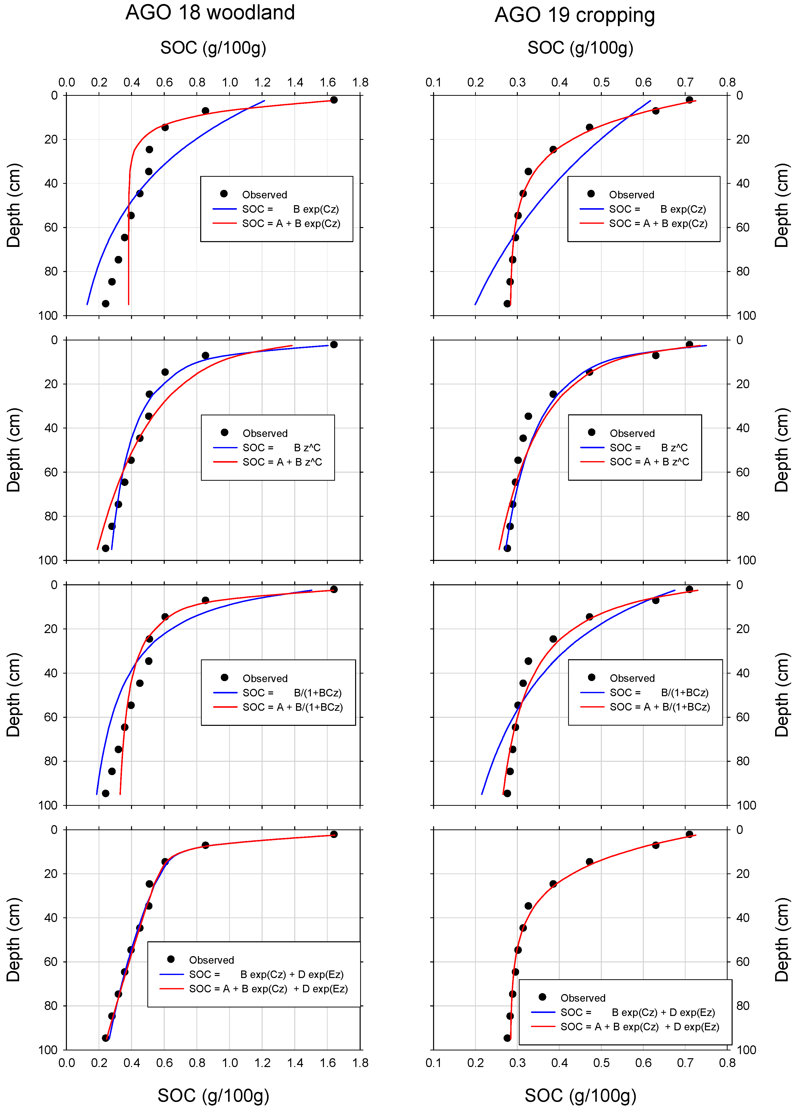
3.1. Statistical Fitting of Functions

The summary of the goodness of fit of the different mathematical functions to the 85 SOC profiles is shown on

Table 3. Mathematical models of the depth distribution of SOC for different land uses. Standard Error of Estimate (SEE) and adjusted R² of fits of functions to 85 data sets of SOC distributions to ≈100 cm from NSW Australia. Moreover, mean values for parameters of equations where the optimisation process converged and the mathematical functions could be fitted to the data, are included. The symbol “–“ indicates that the parameter does not occur in the model.

Model	Equation Number. (See Table 1)	Land Use	Number of Profiles Fitted	% Profiles Fitted	MeanSEE	Mean adj R2	10th Percentile Adj R2	90th Percentile Adj R2	Term Values
									A	B	C	D	E
1 Exponential	6	Cropping	16	100	0.120	0.90	0.68	0.99	–	1.660	−0.039	–	–
SOC = B exp (Cz)		Pasture	33	100	0.202	0.91	0.83	0.99	–	2.675	−0.080	–	–
		Woodland	36	100	0.329	0.91	0.77	0.99	–	4.881	−0.081	–	–
2 Exponential	7	Cropping	15	94	0.073	0.98	0.94	0.99	0.150	1.729	−0.067	–	–
SOC = A + B exp (Cz)		Pasture	33	100	0.110	0.97	0.93	0.99	0.245	2.750	−0.125	–	–
		Woodland	36	100	0.155	0.97	0.77	0.99	0.402	5.108	−0.128	–	–
3 Two-phase exponential	8	Cropping	15	94	0.056	0.99	0.96	0.99	–	1.880	−0.227	0.690	−0.016
SOC = B exp (Cz) + D exp (Ez)		Pasture	31	94	0.090	0.98	0.91	0.99	–	2.815	−0.192	0.690	−0.013
		Woodland	35	97	0.118	0.99	0.95	0.99	–	5.243	−0.200	0.934	−0.012
4 Two-phase exponential	9	Cropping	14	88	0.065	0.98	0.94	0.99	0.047	1.706	−0.273	0.937	−0.025
SOC = A + B exp (Cz) + D exp (Ez)		Pasture	27	82	0.106	0.96	0.87	0.99	0.140	5.403	−0.427	0.861	−0.035
		Woodland	25	69	0.159	0.97	0.90	0.99	0.082	5.496	−0.217	2.122	−0.024
5 Power	10	Cropping	16	100	0.151	0.87	0.62	0.96	–	2.578	−0.451	–	–
SOC = B zC		Pasture	33	100	0.161	0.94	0.84	0.99	–	4.024	−0.603	–	–
		Woodland	36	100	0.208	0.96	0.90	0.99	–	7.914	−0.661	–	–
6 Power	11	Cropping	9	56	0.108	0.89	0.20	0.99	−1.550	4.273	−0.287	–	–
SOC = A + B zC		Pasture	31	94	0.114	0.97	0.90	0.99	−0.301	3.802	−0.424	–	–
		Woodland	34	94	0.179	0.99	0.91	0.99	−0.724	8.310	−0.534	–	–
7 Inverse	12	Cropping	16	100	0.096	0.93	0.79	0.99	–	2.145	0.050	–	–
SOC = B/(B + Cz)		Pasture	33	100	0.123	0.96	0.93	0.99	–	4.115	0.071	–	–
		Woodland	33	92	0.176	0.97	0.91	0.99	–	6.147	0.048	–	–
8 Inverse	13	Cropping	16	100	0.070	0.96	0.85	0.99	−0.233	2.835	0.058	–	–
SOC = A + B/(B + Cz)		Pasture	33	100	0.103	0.97	0.93	0.99	−0.038	4.504	0.081	–	–
		Woodland	32	89	0.152	0.98	0.93	0.99	−0.026	8.609	0.055	–	–

. The average goodness of fit was evaluated for each general land use, cropping, pasture and woodland. The simple exponential functions (Equations (5) and (6)) consistently produced the overall best fit for the depth distributions of SOC, and unlike the two-phase exponential functions (Equations (7) and (8)), all SOC profiles could be fitted. For Equation (6), all adjusted R² values were more than 0.90 and had the lowest SEE. The inclusion of the A term (Equation (6)) in the function improved the goodness of fit of the function to the SOC profiles.

The two-phase exponential functions (Equations (7) and (8)) fitted the SOC profiles well when they could be fitted to the data. For Equation (7), the R² values were always more than 0.90 and the SEE was low. However, there were some difficulties in fitting some of the SOC profiles, and only 94% to 97% of the profiles could be fitted to Equation (7), but with the inclusion of the A term (Equation (8)) only 69% to 88% of the profiles could be fitted to the function. On occasions, the A parameter was estimated to be zero, thereby simplifying Equation [8] to an equivalent Equation (7). Other instances occurred where the A and B (or D) parameter was estimated to be zero, suggesting that the more succinct Equations (5) or (6) were appropriate. In other cases, models simply failed to converge. The large number of estimated parameters in the function (five) was probably a factor when the function could not be fitted to some of the SOC profiles.

The simple power function (Equation (9)) performed well, but not as well as Equation (6) (simple exponential with an A term). The power function with an A term (Equation (10)) performed poorly for the soils under cropping. Many SOC profiles failed to fit the function, especially in the cropping land use and the R² values were low. Under pasture and woodland, Equation (10) performed slightly better than the simple power function. The reason for the difference appears to be that for the sites under cropping, the function overestimated the SOC at the surface, and therefore, this prevented the function from converging to the measured data. The soils under cropping had low SOC at the soil surface.

The inverse functions (Equations (11) and (12)) performed reasonably well for the soils under cropping and pasture, with all SOC profiles being fitted and the R² and SEE values being comparable to the simple exponential functions. However, the inverse functions failed to fit 8.3% (Equation (11)) to 11.1% (Equation (12)) of SOC profiles under woodlands.

The single-phase exponential function with an A term (Equation (6)) performed best overall, but even these functions showed sections of the SOC profile where the function did not fit the data. The two-phase exponential functions showed some potential to fit the SOC profile data very well, particularly in soils and land-uses where there was a larger surface SOC concentration, but a substantial number of SOC profiles failed to fit the function.

An example of how the functions fitted the measured data is shown in

Table 4. Mathematical models of the depth [z cm] distribution of SOC for each of a set of paired sites on Grey Vertosols on the Darling Riverine Plain in north Western NSW [AGO sites 18 and 19]. Example of goodness of fit of functions and influence of land use [cropping versus woodland]. Graphs for these are shown in Figure 4. “–“ indicates that the parameter does not occur in the model. Equation numbers refer to Equations in text and Table 1.

Model	Equation See Text	Land Use	SOC Profile Number	SEE	Adj R2	Estimated Model Parameters
						A	B	C	D	E
5 Exponential	5	Cropping	AGO 19	0.069	0.79	-	0.636	−0.0122	-	-
SOC = B exp (Cz)		Woodland	AGO 18	0.213	0.71	-	1.290	−0.0244	-	-
6 Exponential	6	Cropping	AGO 19	0.012	0.99	0.282	0.518	−0.0629	-	-
SOC = A + B exp (Cz)		Woodland	AGO 18	0.095	0.94	0.382	1.837	−0.1582	-	-
7 Two-phase exponential	7	Cropping	AGO 19	0.013	0.99	-	0.518	−0.0630	0.283	0.0000
SOC = B exp (Cz) + D exp (Ez)		Woodland	AGO 18	0.017	0.99	-	2.069	−0.3040	0.695	−0.0102
8 Two-phase exponential	8	Cropping	AGO 19	0.014	0.99	0.282	0.3255	−0.0624	0.1925	−0.0636
SOC = A + B exp (Cz) + D exp (Ez)		Woodland	AGO 18	0.013	0.99	−1.243	2.047	−0.2836	1.8923	−0.0025
9 Power	9	Cropping	AGO 19	0.033	0.95	-	0.969	−0.2789	-	-
SOC = B zC		Woodland	AGO 18	0.052	0.98	-	2.494	−0.4821	-	-
10 Power	10	Cropping	AGO 19	0.032	0.96	−0.550	1.443	−0.1282	-	-
SOC = A + B zC		Woodland	AGO 18	0.046	0.99	1.163	2.619	−0.6303	-	-
11 Inverse	11	Cropping	AGO 19	0.048	0.90	-	0.717	0.0343	-	-
SOC = B/(1 + B * Cz)		Woodland	AGO 18	0.131	0.89	-	1.860	0.0510	-	-
12 Inverse	12	Cropping	AGO 19	0.021	0.98	0.196	0.650	0.1343	-	-
SOC = A + B/(1 + B * Cz)		Woodland	AGO 18	0.055	0.98	0.270	3.293	0.1709	-	-

and Figure 4 for a woodland site (AGO 18) and a cropping site (AGO 19). This was a paired site on a Grey Vertosol on the Darling Riverine Plain in north western NSW. The function that was closest to fitting all the measured data points in the SOC profile was the two-phase exponential function (Equation (8)) for both the woodland and the cropping sites. This is consistent with the fit of the single exponential phase function substantially improving when a constant (A) was added to the function (Equation (6) in Table 4)], which at least partially takes account of the two-phase nature of the SOC profiles. The functions generally seem to fit better overall to the measured data in the SOC profile for the cropping site than the woodland site.

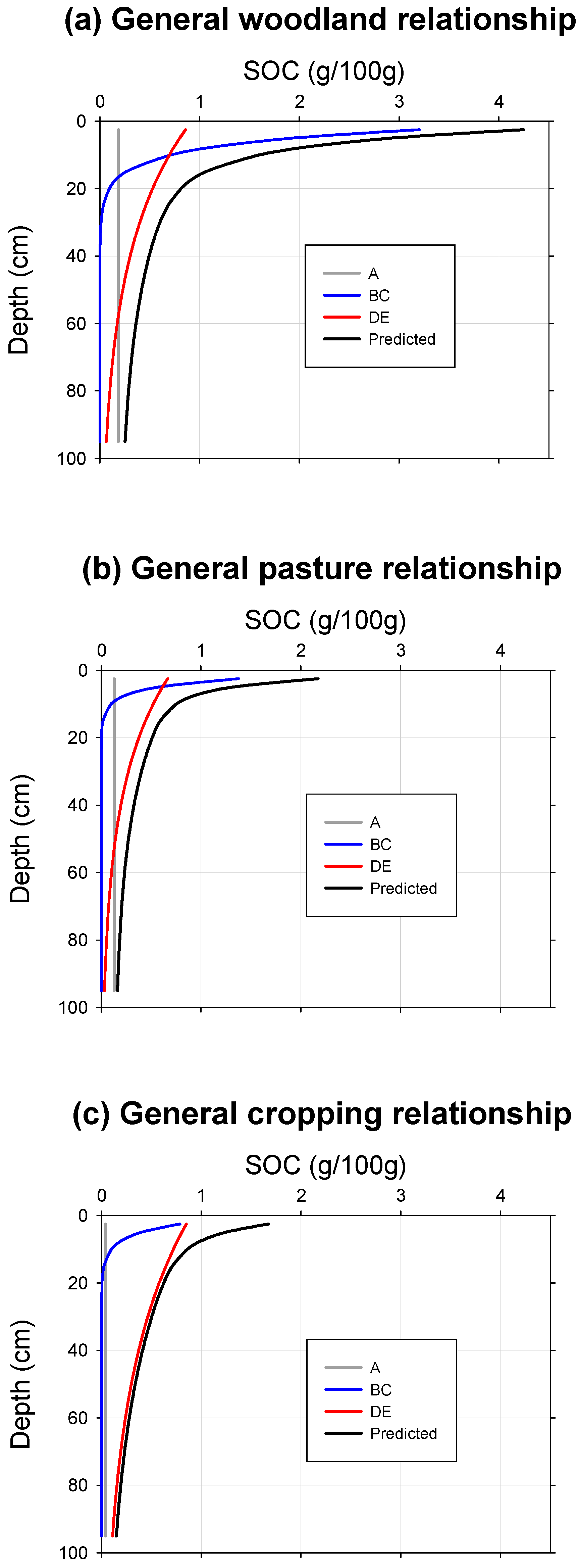
3.2. Interpretation of the Two-Phase Exponential Function

The mean parameter values of the two-phase exponential function from Table 3 are shown in Figure 5. The depth distributions clearly show the occurrence of at least two phases of “processes” in the SOC profiles. The first was a shallow phase that appears to control the high amounts of SOC in the surface soils and this decreases rapidly with depth. The second was a process controlling lower amounts of SOC, but this extends for much deeper into the soil profile. The results for the two-phase exponential function do provide evidence for the occurrence of different phases or sets of processes in the SOC profiles as hypothesized in Section 1.2.

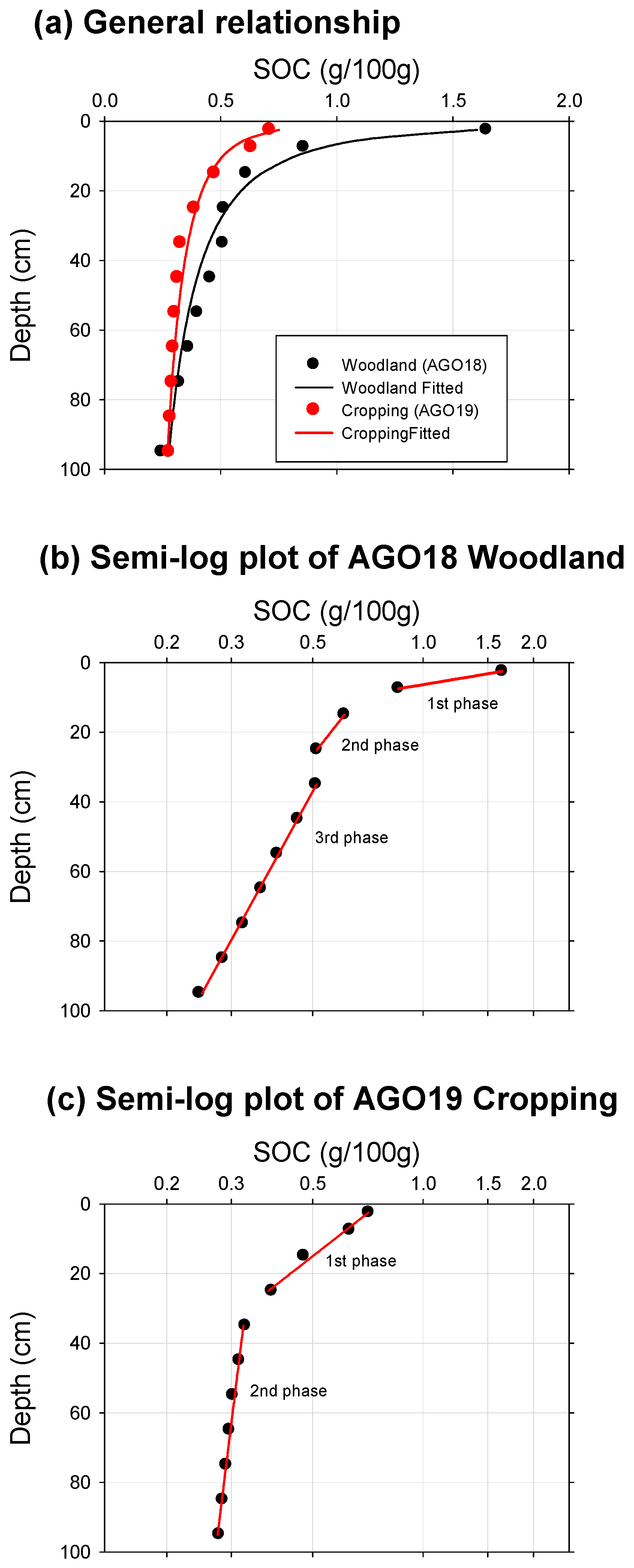
3.3. Semi-Log Plots of SOC v’s Depth

Semi-log plots have often been used to detect relationships between variables, especially if exponential relationships are expected. The results of some of the semi-log plots for the SOC profiles are shown in

Table 5. Relationships based on semi-log plots and two-phase exponential functions for several SOC profiles with different paired land uses.

Semi Log Plot: Segments Fitted as loge(SOC) = b + mz; Backtransformed as G = exp (b)						Two Phase: Fitted as SOC = A + B exp (Cz) + D exp (Ez)
Phase	Depth [cm]	G	m	SEE	R2	Parameter Estimates		SEE	R2
AGO 18; Land use = woodland; n = 11. Paired site with AGO 19
a	0–7.5	2.278	−0.1302	0.013	0.99	B = 2.048	C = −0.2877	0.013	0.998
b	15–25	0.790	−0.0172			D = 1.892	E = −0.0025
c	35–95	0.781	−0.0120			A = -1.243
AGO 19; Land use = cropping; n = 11. Paired site with AGO 18
a	0–25	0.760	−0.0279	0.025	0.99	B = 0.325	C = −0.0624	0.014	0.99
b	35–95	0.356	−0.0027			D = 0.193	E = −0.0636
						A = 0.282
AGO 14; Land use = woodland; n = 11. Paired site with AGO 15
a	0–7.5	3.667	−0.1742	0.032	0.99	B = 47.110	C = −1.4822	0.060	0.99
b	15–35	1.831	−0.0435			D = 1.252	E = −0.0319
c	45–75	0.806	−0.0180			A = 0.068
d	85–95	4.862	−0.0407	Front of added SOC
AGO 15; Land use = cropping; n = 11. Paired site with AGO 14
a	0–35	1.335	−0.0397	0.033	0.99	B = 1.134	C = −0.0509	0.024	0.99
b	35–95	0.615	−0.0176			D = 0.192	E = −0.0077
						A = 0.025
Bingara–Yeral/Pinetrees–woodland; n = 9
a	0–7.5	6.416	−0.1695	0.328	0.70	B = 82.436	C = −1.4947	0.234	0.94
b	15–35	1.656	−0.0155			D = 1.715	E = −0.0687
c	45–55	0.506	0.0112			A = 0.789
d	65–75	70.142	−0.0654	Front of added SOC
Bingara–Yeral/Pinetrees–pasture; n = 11
a	0–7.5	2.756	−0.0904	0.346	0.84	B = 13.089	C = −1.2287	0.141	0.94
b	15–95	1.515	−0.0229			D = 1.694	E = −0.0244
						A = −0.001
Bingara–Yeral/Pinetrees–cropping; n = 11
a	0–15	2.223	−0.0761	0.129	0.97	B = 1.715	C = −0.1113	0.059	0.98
b	25–55	0.895	−0.0205			D = 0.448	E = −0.0133
c	65–95	0.326	−0.0039			A = 0.088
Guyra Basalt–Woodland; n = 10
a	0–7.5	10.276	−0.1342	0.111	0.99	B =9.355	C=−0.3397	0.604	0.99
b	15–35	3.322	−0.0188			D=4.978	E =−0.0145
c	45–65	6.741	−0.0411	Front of added SOC		A=−1.450
d	75–85	271.106	−0.0967	Front of added SOC
Guyra Basalt–Pasture; n = 10
a	0–7.5	6.329	−0.0628	0.111	0.99	B = 2.433	C =−0.1637	0.197	0.99
b	15–35	3.987	−0.0350			D = 4.248	E = −0.0400
c	45–85	2.276	−0.0318			A = −0.023
Guyra Basalt–Cropping; n = 10
a	0–7.5	4.821	−0.0747	0.237	0.95	B = 3.204	C = −0.1273	0.115	0.99
b	15–25	2.720	−0.0334			D = 1.877	E = −0.0226
c	35–85	2.049	−0.0285			A = −0.098
AGO Site 16–Woodland; n = 11
a	0–7.5	4.428	−0.1305	0.113	0.99	B = 3.972	C = −0.2904	0.192	0.96
b	15–45	1.340	−0.0135			D = 25.373	E = −0.0005
c	55–75	5.564	−0.0332	Front of added SOC		A = −24.069
d	85–95	>>200	−0.1837	Front of added SOC
AGO Site 17–Cropping; n = 11
a	0–7.5	1.001	−0.0498	0.043	0.99	No fit
b	15–45	0.731	−0.0012			No fit
c	55–75	5.569	−0.0361	Front of added SOC		No fit
d	85–95	>>200	−0.2680	Front of added SOC

and Figure 6. Note that to detect the segmented relationships between SOC and depth, log_e(SOC) was plotted on the y-axis and the depth on the x-axis. The results of the semi-log plots show that for SOC profiles examined, there were at least two distinct relationships between SOC and depth, each relationship having different values for the terms in the exponential equation. This indicates that it is unlikely that a single relationship can explain all the points of the SOC distribution, which is consistent with the observation for most of the SOC profiles, that when using the functions in Table 1 and Table 3, at least some observed values of SOC do not fit the fitted function. The R² and SEE for the relationships derived using the semi-log plots are shown in Table 5 and show that it is possible to fit the observed values better using the relationship derived from the semi-log plots.

3.4. Comparison of Results from Two-Phase Exponential Functions and Semi-Log Plots

The analysis using the two-phase exponential functions and the semi-log plots showed a relationship for the shallow soils (<10 to 20 cm) and relationship with different values for the terms of the equations for deeper soils (>30 cm). A comparison of the functions derived from the SOC profiles showed that there was some variation between those derived for the two-phase exponential and those derived from the semi-log plots (Figure 7a,b). The shallow phase for the two-phase exponential functions was shallower and had higher decline values than those observed using the semi-log plots (Table 5) and Figure 6. For example, the rate of decline with depth (C) for the woodland site AGO 18 was −0.300 compared to the rate measured using the semi-log plots of −0.1302. The values for the terms in the two-phase exponential functions are based on an analysis of the whole profile, whereas the surface soil functions derived using the semi-log plots are based on the surface data alone, thus, it is difficult to compare the values. For the paired cropping site (AGO 19), the rate of decline with depth (C) was −0.064 for the two-phase exponential and −0.028 for the semi-log plot. The distribution of SOC at the surface reflects a relationship that is a composite of the near surface processes and possibly some ”background” store of SOC. It is possible the two-phase exponential functions reflect the surface processes more strongly, because it is based on data from the whole profile.

4. Discussion

4.1. General

The evidence from fitting the mathematical functions and the semi-log plots to the SOC profiles strongly supports our hypothesis that there are several zones in the soil where different processes are influencing the SOC profiles. Most of the SOC profiles show at least two clear phases in the SOC profile. This is consistent with the model proposed by Gross and Harrison [47], who identified two clear zones in the depth distribution of SOC, with a surface layer where shoot inputs > root inputs and a deeper layer where root inputs > shoot inputs. Gross and Harrison suggested that shoot inputs are commonly significant for the top 10 cm of soil, although this can be slightly deeper in forest soils. They identified that the rhizosphere is an important source of organic carbon for SOC, and the organic carbon in the rhizosphere is often modified by microbial processes, much more so than the organic carbon from shoot materials. The dominant, overall effect is the exponential distribution with depth which reflects the root distribution. However, this appears in many cases to show a stronger effect of the roots on SOC in the upper profile [<40–50 cm] where fine root turnover and root exudates can be expected to have a larger effect on SOC [50,64]. This is also the zone where soil fauna activity, bioturbation and microbial activity are strongest [15,34,49]. Several SOC profiles showed a strong near surface soil phase, especially the profiles from soils with higher surface SOC concentration under woodland soils and some pasture soils. Below 50 cm, many SOC profiles show a “baseline” level of SOC which indicates a deep soil level of SOC that remains perhaps more stable and where there is a lower level of input from fine roots and root exudates. In some soil profiles, a layer deeper in the soil [>80 cm] occurs where there are very low levels of SOC [<0.1%] and perhaps indicating that root growth is very restricted in these layers. Advection or transport of dissolved SOC in liquid flow can also add to SOC stocks in deeper soils [34].

The exponential functions that fitted most successfully to the SOC profiles were the simple exponential with an A constant and the two-phase exponential functions. Sometimes, the two-phase exponential function with an A constant could not be fitted or the A term was 0. However, the success of these functions in fitting the SOC profiles supports the existence of at least two phases within the SOC profiles. With the simple exponential function with the A constant, the exponential term accounted for one phase, including the surface layer phase, and the A term the deeper “background” phase (see Figure 5 and Figure 6). However, the simple exponential function without the A constant generally did not fit the SOC profiles a well as the other exponential functions. As this function can only account for one phase in the SOC profile, this is evidence that the SOC profiles do show at least two phases in their depth profiles.

In the two-phase exponential function, the first exponential term accounted for the surface soil phase and the second exponential term the deeper soil phase. Semi-log plots clearly identified different phases in the SOC profiles. This was particularly true where there was a more significant accumulation of SOC in surface soil layers creating a non-symmetrical curve. However, where this surface SOC accumulation diminished, the second exponent term tended to zero at which point a typical one phase exponential function was adequate to describe the distribution. Some SOC profiles only had two phases, some three, but some profiles had up to four for a range of reasons (see below for complex profiles). Where three phases were detected, the two-phase exponential function with the A constant, the A term accounted for the deeper soil “depth independent” or “background” SOC.

While the power functions and the Inverse functions were fitted to the SOC profiles with some success, they did not fit as well as the exponential based functions. Additionally, the biophysical basis for choosing these functions is lacking and does not have the strong case that applies to the exponential functions. Therefore, these are no longer considered.

Some SOC profiles showed complex distributions that did not follow clear relationships and the functions showed a poor fit or could not be fitted. Profiles AGO 16 and 17, adjacent soils from a paired site, are examples (Figure 8). These SOC profiles maintained substantial amounts of SOC deep into the profile (to 50 cm) or showed substantial increases in SOC at 50 cm. The nature of the native vegetation and land use history may have had an influence on these soils [76]. The native trees are Myall [Acacia pendula], an N-fixing tree, with an above ground biomass of 85 to 90 Mg ha⁻¹. The understory consisted of plants from the Chenopodiaceae [saltbush] and various grasses including curly windmill grass (Enteropogon acicularis) and Wallaby Grass (Austrodanthonia linkii). The understory had a biomass of 12.7 Mg ha^-1 when the samples were taken for the SOC profile. It is speculated that this may have contributed to the non-standard nature of this SOC profile. A standard SOC profile has a decreasing rate of decline in SOC with depth, which means a decreasing value of “m” in Equation (13).

The SOC profiles in AGO 16 and 17 had some features of the “wetting front” typology of depth functions described by Minasny et al. [22], characterized by an increasing rate of decline in SOC with depth or an increase in the value of “m” from Equation [13] with depth. Such SOC profile is consistent with the accumulation and movement of SOM into the soil in association with root growth from active grass species and Chenopod species, possibly supported by N fixation by the Acacia species.

The woodland sites in the Guyra basalt and Bingara metasediments also showed a similar “wetting front” typology for the SOC profile, as can be seen by the very high G values for the deep phases of the SOC profile derived using the semi-log plots [Table 5; Figure 7d and Figure 8]. The implication is that both these woodland sites have accumulating profiles of SOC.

4.2. Effects of Land Use

The nature of the SOC profiles for cropping, pasture and woodland showed some quite different characteristics [see Figure 5 and Figure 6]. The near surface phase of the SOC profile was much stronger or pronounced in the soils under woodland with higher inputs of shoot material at the surface [45,52,76,85]. Some of the woodland sites, particularly AGO 16 and that on the Bingara metasediments showed a “wetting front” typology as defined by Minasny et al. [22], indicating an accumulation of SOC to depth [>50 cm] and the SOC profile did not follow a standard decrease in the rate of decline in SOC with depth. At the depth of accumulation there was a pronounced increase in the rate of decline of SOC with depth, typical of a “wetting front” typology [see Figure 8]. The woodland sites showed a higher amount of SOC to a depth generally more than 30 cm, which is the standard depth for estimating SOC stocks.

Soils under cropping had simpler SOC profiles and generally could be fitted to functions more easily than those under woodland or pasture land use. The near surface phase of the SOC profiles was less pronounced and a pronounced near surface phase in the SOC profile may have been absent. A general effect was that there was an underlying baseline of SOC deeper in the profile that had an approximate common value for SOC, although this could vary somewhat. Soils under pasture were intermediate between cropping and woodlands, showing some near surface phases, but not as pronounced as the woodlands [45]. The overall conclusion was that land use clearly had an influence on the processes controlling the SOC profiles at different depths. The occurrence of different processes occurring at different depth phases within the SOC profiles of soils was largely supported by the SOC profiles. The use of semi-log plots may provide a method to examine more closely some of the data on specific cropping practices such as stubble retention and minimum tillage.

4.3. Modelling SOC Profiles

The best fit was usually the single-phase exponential function with an A term or the two-phase exponential function where there was a significant SOC accumulation at the surface. The best fit was found typically where it was possible to account for at least two phases in the SOC profile, either by using a constant as in A, or as a two-phase exponential function. The limitation of using the two-phase exponential function is its difficulty of computation and the common possibility of not being able to find a fit because of the high number of terms in the equation relative to the potentially available data points or degrees of freedom.

The best predictions were obtained using the development of the relationships from the semi-log plots with R² for the SOC profiles investigated of more than 0.98 [see Table 5] and square root of the Error Mean Square (SEE) nearly always <0.1. Effectively, a similar process to fitting data using spline functions, but potentially has a more meaningful biophysical basis.

While the R² value for the relationships were often high and the RMSE is low for many SOC profiles, in general, for some SOC profiles the mathematical functions were good approximations at best to the actual SOC profiles (see Table 3 and Figure 4). As can be seen from Site 16 and 17 (Figure 8), even though the R² is 0.94 and the RMSE is 0.14, there are still a number of observations within the SOC profile where the mathematical function did not precisely fit the observation.

However, there, functions tended to fail when the depth distribution of SOC does not show simple rates of decrease in SOC with depth. The conclusion is that there are more complex processes controlling the depth distribution of SOC. In these SOC profiles there are fronts of SOC accumulation or indications of buried profiles and unusual accumulations of SOC at depth. Some of these profiles are shown in Figure 8.

4.4. Implications for Management and Policy

The SOC profiles and their relationship to the mathematical functions have several implications for the development of the understanding of the sequestration of SOC and the inputs of carbon into the soil.

• At least two phases and sets of processes operating at different depths in the soil, and these are influenced by land use and soil type. A general implication of this is that it suggests a single measurement of SOC over a depth of 30 cm is going to contain soil materials with a wide range of SOC concentrations. Effective homogenization of the bulked sample before subsampling is an essential step in the measurement of SOC content and SOC stocks.
• Surface input of carbon is important under some land uses, especially woodlands, but less important under cropping, although stubble retention may provide limited amounts of biomass to the surface soils. The apparent failure of many stubble retention trials with direct drilling to increase SOC can be partially explained by the low level of shoot inputs provided by stubble retention and the lack of mechanisms to transport organic materials deeper into the profile [86]. The use of semi-log plots and a finer scale of SOC measurements with depth may provide a better understanding of the effects of direct drilling and stubble retention on the dynamics of SOC.
• SOC deeper in the subsoil can be subject to several inputs, but roots are probably the major source, even in Vertosols. Advection can transport dissolved SOC in liquid flow into the deeper subsoil [34], but given the drier climate associated with many of the soils, the amount of flow into the deeper soils is limited.
• At least three phases have been identified in the SOC profiles, near surface, mid depth and deep or baseline SOC. These have been identified by the nature of the SOC profiles [see Figure 5 and Figure 6]. In promoting land management practices to sequester carbon, an understanding of these phases is helpful. Woodland or native vegetation increases SOC in near surface layers, pasture in subsurface layers and the baseline or deep carbon is more difficult to influence. Cropping does not promote increases in SOC near surface. This is potentially a method to investigate the effects of different land management practices on SOC profiles.

The terms in the functions can be used to identify the relative importance of different phases in the SOC profiles [see Figure 6, Figure 7 and Figure 8]. The functions can identify the amount of SOC associated with near surface processes and the amount of SOC in the deeper profile. It can also identify the presence of SOC fronts of accumulation [see Table 5] from semi-log plots.

5. Conclusions

Simple mathematical functions can be used to predict the SOC profiles for many soils. Of these Equation 6 which is an exponential function with a constant is the most reliable. Two phase exponential functions are also very effective to predict SOC profiles, particularly where larger quantities of surface SOC are present, but have the limitation of sometimes being difficult to fit to more complex SOC profiles. In these cases, the degrees of freedom or measurements become a limitation. The two-phase exponential functions have four to five terms that need to be fitted to a data set which can limit their application for many SOC profiles. The power and inverse functions, while useful, were generally inferior to the exponential functions and have an uncertain biophysical basis.

The analysis of the SOC profiles confirmed that many SOC profiles demonstrate at least two and sometimes up to four zones within the SOC profiles where different processes dominate. This was often evident within the data and in applying the mathematical functions to the SOC profiles. The two-phase exponential functions clearly demonstrated the occurrence of at least two and sometimes three phases in the SOC profiles. An analysis using semi-log plots demonstrated the occurrence of zones within the SOC profiles. The use of semi-log plots is a potential tool to identify the processes occurring in the SOC profiles in soils and so potentially can be used to identify the effects of land management practices on SOC sequestration and storage in more detail.

Several SOC profiles demonstrated specific features that are potentially important for the management of SOC profiles in soils. Woodland and to lesser extent pasture soils had a definite near surface zone within the SOC profile, indicating the addition of surface materials and high rates of fine root turnover. This zone was much less evident under cropping. Several SOC profiles showed evidence for a front of SOC accumulation moving down the profile and did not have the definite rate of decline of SOC with depth that was more commonly observed. These were typically soils under a woodland land use.

References

1. Baldock, J.A.; Skjemstad, J.O. Soil organic carbon/Soil organic matter. In Soil Analysis—An Interpretation Manual; Peverill, K.I., Sparrow, L.A., Reuter, D.J., Eds.; CSIRO Publishing Collingwood Australia: Collingwood, Australia, 1999. [Google Scholar]
2. Lal, R. Soil carbon sequestration to mitigate climate change. Geoderma 2004, 123, 1–22. [Google Scholar] [CrossRef]
3. Department of Environment. Carbon Credits (Carbon Farming Initiative) Sequestering Carbon in Soils in Grazing Systems Methodology Determination 2014. Methodology Determination under subsection 106(1) Carbon Credits (Carbon Farming Initiative Act 2011, Department of Environment. Australian Government. 2014; Available online: http://www.environment.gov.au/node/37951 or http://www.comlaw.gov.au/Details/F2014L00987; (accessed on 29 May 2019). [Google Scholar]
4. Batjes, N. Total carbon and nitrogen in the soils of the world. Eur. J. Soil Sci. 1996, 47, 151–163. [Google Scholar] [CrossRef]
5. Minasny, B.; Malone, B.P.; McBratney, A.B.; Angers, D.A.; Arrouays, D.; Chambers, A.; Chaplot, V.; Zueng-Chen, S.; Chengg, K.; Das, B.S.; et al. Soil carbon 4 per mille. Geoderma 2017, 292, 59–86. [Google Scholar] [CrossRef]
6. Luo, Z.; Wang, E.; Sun, O.J. Soil carbon change and its responses to agricultural practices in Australian agro-ecosystems: A review and synthesis. Geoderma 2010, 155, 211–223. [Google Scholar] [CrossRef]
7. Sombroek, W.G.; Nachtergaele, F.O.; Hebel, A. Amounts, dynamics and sequestering of carbon in tropical and subtropical soils. Ambio. Stockh. 1993, 22, 417–426. [Google Scholar]
8. IPCC. Chapter 5 Land Use Change and Forestry. Revised 1996 Guidelines for National Greenhouse Gas Inventories. International Panel on Climate Change. 1996. Available online: https://www.ipcc-nggip.iges.or.jp/public/gl/invs4.html (accessed on 29 May 2019).
9. Wendt, J.W.; Hauser, S. An equivalent soil mass procedure for monitoring soil organic carbon in multiple soil layers. Eur. J. Soil Sci. 2013, 64, 58–65. [Google Scholar] [CrossRef]
10. Bonfatti, B.R.; Hartemink, A.E.; Giasson, E. Comparing Soil C Stocks from Soil Profile Data Using Four Different Methods. In Progress in Soil Science; Springer Science and Business Media LLC: Cham, Switzerland, 2016; pp. 315–329. [Google Scholar]
11. Russell, J.; Moore, A. Comparison of different depth weightings in the numerical analysis of anisotropic soil profile data. In Proceedings of the Transactions of the 9th International Congress of Soil Science, 5–15 August 1968; pp. 205–213. [Google Scholar]
12. Kirkby, M.J. Soil development models as a component of slope development models. Earth Surf. Process. 1977, 2, 203–230. [Google Scholar] [CrossRef]
13. Dalal, R.C.; Chan, K.Y. Soil organic matter in rainfed cropping systems of the Australian cereal belt. Soil Res. 2001, 39, 435. [Google Scholar] [CrossRef]
14. Kempen, B.; Brus, D.; Stoorvogel, J.; Stoorvogel, J. Three-dimensional mapping of soil organic matter content using soil type–specific depth functions. Geoderma 2011, 162, 107–123. [Google Scholar] [CrossRef]
15. Meersmans, J.; Van Wesemael, B.; De Ridder, F.; Van Molle, M. Modelling the three-dimensional spatial distribution of soil organic carbon (SOC) at the regional scale (Flanders, Belgium). Geoderma 2009, 152, 43–52. [Google Scholar] [CrossRef]
16. Wiese, L.; Ros, I.; Rozanov, A.; Boshoff, A.; De Clercq, W.; Seifert, T. An approach to soil carbon accounting and mapping using vertical distribution functions for known soil types. Geoderma 2016, 263, 264–273. [Google Scholar] [CrossRef]
17. Lorenz, K.; Lal, R. The Depth Distribution of Soil Organic Carbon in Relation to Land Use and Management and the Potential of Carbon Sequestration in Subsoil Horizons. Adv. Agron. 2005, 88, 35–66. [Google Scholar]
18. Bolinder, M.A.; Janzen, H.H.; Gregorich, E.G.; Angers, D.A.; Vandern Bygaart, A.J. An approach for estimating net primary productivity and annual soil carbon inputs to soil for common agricultural crops in Canada. Agric. Ecosyst. Environ. 2007, 118, 29–42. [Google Scholar] [CrossRef]
19. Newey, A. Decomposition of Plant Litter and Carbon Turnover as a Function of Soil Depth. Ph.D. Thesis, Australian National University, Canberra, Australia, 2005. [Google Scholar]
20. Don, A.; Rödenbeck, C.; Gleixner, G. Unexpected control of soil carbon turnover by soil carbon concentration. Environ. Chem. Lett. 2013, 11, 407–413. [Google Scholar] [CrossRef]
21. Wordell-Dietrich, P.; Don, A.; Helfrich, M. Controlling factors for the stability of subsoil carbon in a Dystric Cambisol. Geoderma 2017, 304, 40–48. [Google Scholar] [CrossRef]
22. Minasny, B.; Stockmann, U.; Hartemink, A.E.; McBratney, A.B. Chapter 14. Measuring and Modelling Soil Depth Functions. In Digital Soil Morphometrics; Progress in Soil, Science; Hartemink, A.E., Minasny, B., Eds.; Springer International Publishing: Cham, Switzerland, 2016. [Google Scholar]
23. Mikhailova, E.; Bryant, R.; Vassenev, I.; Schwager, S.; Post, C. Cultivation Effects on Soil Carbon and Nitrogen Contents at Depth in the Russian Chernozem. Soil Sci. Soc. Am. J. 2000, 64, 738. [Google Scholar] [CrossRef]
24. Grauer-Gray, J.; Hartemink, A.E. Raster sampling of soil profiles. Geoderma 2018, 318, 99–108. [Google Scholar] [CrossRef]
25. Wong, V.N.L.; Murphy, B.W.; Koen, T.B.; Greene, R.S.B.; Dalal, R.C. Soil organic carbon stocks in saline and sodic landscapes. Soil Res. 2008, 46, 378–389. [Google Scholar] [CrossRef]
26. Hobley, E.U.; Wilson, B. The depth distribution of organic carbon in the soils of eastern Australia. Ecosphere 2016, 7, e01214. [Google Scholar] [CrossRef] [Green Version]
27. International Union of Soil Science Working Group WRB [IUSS]. World Reference Base for Soil Resources 2014, Update 2015: International Soil Classification System for Naming Soils and Creating Legends for Soil Maps; World Soil Resources Reports No. 106; FAO: Rome, Italy, 2015. [Google Scholar]
28. Gerwitz, A.; Page, E.R. An Empirical Mathematical Model to Describe Plant Root Systems. J. Appl. Ecol. 1974, 11, 773. [Google Scholar] [CrossRef]
29. King, J.; Gay, A.; Sylvester-Bradley, R.; Bingham, I.; Foulkes, J.; Gregory, P.; Robinson, D. Modelling cereal root systems for water and nitrogen uptake: Towards an economic optimum. Ann. Bot. 2003, 91, 383–390. [Google Scholar] [CrossRef] [PubMed]
30. Zuo, O.; Fie, F.; Zhang, R.; Meng, L. A Generalized Function of Wheat’s Root Length Density Distributions. Vadose Zone J. 2004, 3, 271–277. [Google Scholar] [CrossRef]
31. Porter, J.R.; Klepper, B.; Belford, R.K. A model (WHTROOT) that synchronises root growth and development with shoot development in winter wheat. Plant Soil 1986, 92, 133–145. [Google Scholar] [CrossRef]
32. Jobbágy, E.G.; Jackson, R.B. The vertical distribution of soil organic carbon and its relation to climate and vegetation. Ecol. Appl. 2000, 10, 423–436. [Google Scholar]
33. Neff, J.C.; Asner, G.P. Dissolved Organic Carbon in Terrestrial Ecosystems: Synthesis and a Model. Ecosystems 2001, 4, 29–48. [Google Scholar] [CrossRef] [Green Version]
34. Braakhekke, M.C.; Wutzler, T.; Beer, C.; Kattge, J.; Schrumpf, M.; Ahrens, B.; Schöning, I.; Hoosbeek, M.R.; Kruijt, B.; Kabat, P.; et al. Modeling the vertical soil organic matter profile using Bayesian parameter estimation. Biogeosciences 2013, 10, 399–420. [Google Scholar] [CrossRef] [Green Version]
35. Bishop, T.; McBratney, A.; Laslett, G. Modelling soil attribute depth functions with equal-area quadratic smoothing splines. Geoderma 1999, 91, 27–45. [Google Scholar] [CrossRef]
36. Bernoux, M.; Arrouays, D.; Cerri, C.C.; Bourennane, H. Modeling vertical distribution of carbon in oxisols of the western brazilian amazon (rondonia). Soil Sci. 1998, 163, 941–951. [Google Scholar] [CrossRef]
37. Barson, M.M.; Malafant, K.; Skjemstad, J.O.; Royle, S.; Janik, L.J.; Spouncer, L.R.; Merry, R.H. Estimating the size of Australia’s soil carbon sinks. In Proceedings of the SuperSoil, 3rd Australia New Zealand Soil Conference, Sydney, Australia, 5–9 December 2004. [Google Scholar]
38. Van Cleemput, O.; Carlier, L.; Mestdagh, I.; Lootens, P. Soil organic carbon stocks in Flemish grasslands: How accurate are they? Grass Forage Sci. 2004, 59, 310–317. [Google Scholar]
39. Minasny, B.; McBratney, A.B.; Mendonça-Santos, M.L.; Odeh, I.O.A.; Guyon, B. Prediction and digital mapping of soil carbon storage in the Lower Namoi Valley. Soil Res. 2006, 44, 233–244. [Google Scholar] [CrossRef]
40. Cook, F.J.; Kelliher, F.M. Determining Vertical Root and Microbial Biomass Distributions from Soil Samples. Soil Sci. Soc. Am. J. 2006, 70, 728. [Google Scholar] [CrossRef]
41. Fang, C.; Moncrieff, J.B. The variation of soil microbial respiration with depth in relation to soil carbon composition. Plant Soil 2005, 268, 243–253. [Google Scholar] [CrossRef]
42. Melillo, J.M.; Aber, J.D.; Linkins, A.E.; Ricca, A.; Fry, B.; Nadelhoffer, K.J. Carbon and nitrogen dynamics along the decay continuum: Plant litter to soil organic matter. Plant Soil 1989, 115, 189–198. [Google Scholar] [CrossRef]
43. Whitmore, A.P.; Coleman, K. Use of Rothamsted Carbon model, RothC, in deriving the UK Carbon inventory. In UK Emissions by Sources and Removals by Sinks due to Land Use, Land Use Change and Forestry Activities; DEFRA Contract EPG 1/1/160, CEH No. C02275; Milne, R., Mobbs, D.C., Eds.; Department for the Environment, Food and Rural Affairs, Global Atmosphere Division: London, UK, 2005. [Google Scholar]
44. Minasny, B.; McBratney, A.B.; Malone, B.; Sulaeman, Y. Digital mapping of soil carbon. In Proceedings of the 19th World Congress of Soil Science, Soil Solutions for a Changing World, Brisbane, Australia, 1–6 August 2010. [Google Scholar]
45. Wilson, B.R.; Barnes, P.; Koen, T.; Gosh, S.; King, D. Measurement and estimation of land use effects on soil carbon and related properties on a basalt landscape of northern NSW. Aust. J. Soil Res. 2010, 48, 421–433. [Google Scholar] [CrossRef]
46. Watt, M.; Kirkegaard, J.A.; Passioura, J.B. Rhizosphere biology and crop productivity—A review. Soil Res. 2006, 44, 299. [Google Scholar] [CrossRef]
47. Gross, C.D.; Harrison, R.B. The Case for Digging Deeper: Soil Organic Carbon Storage, Dynamics, and Controls in Our Changing World. Soil Syst. 2019, 3, 28. [Google Scholar] [CrossRef]
48. Gill, R.A.; Burke, I.C. Influence of soil depth on the decomposition of Bouteloua gracilis roots in the shortgrass steppe. Plant Soil 2002, 241, 233–242. [Google Scholar] [CrossRef]
49. Gill, R.; Burke, I.C.; Milchunas, D.G.; Lauenroth, W.K. Original Articles: Relationship Between Root Biomass and Soil Organic Matter Pools in the Shortgrass Steppe of Eastern Colorado. Ecosystems 1999, 2, 226–236. [Google Scholar]
50. Eyles, A.; Coghlan, G.; Hardie, M.; Hovenden, M.; Bridle, K. Soil carbon sequestration in cool-temperate dryland pastures: mechanisms and management options. Soil Res. 2015, 53, 349. [Google Scholar] [CrossRef]
51. Dignac, M.-F.; Derrien, D.; Barré, P.; Barot, S.; Cécillon, L.; Chenu, C.; Chevallier, T.; Freschet, G.T.; Garnier, P.; Guenet, B.; et al. Increasing soil carbon storage: mechanisms, effects of agricultural practices and proxies. A review. Agron. Sustain. Dev. 2017, 37, 351. [Google Scholar] [CrossRef]
52. Leff, J.W.; Wieder, W.R.; Taylor, P.G.; Townsend, A.R.; Nemergut, D.R.; Grandy, A.S.; Cleveland, C.C. Experimental litterfall manipulation drives large and rapid changes in soil carbon cycling in a wet tropical forest. Glob. Chang. Boil. 2012, 18, 2969–2979. [Google Scholar] [CrossRef] [PubMed]
53. Jabiol, B.; Zanella, A.; Ponge, J.-F.; Sartori, G.; Englisch, M.; Van Delft, B.; De Waal, R.; Le Bayon, R.-C. A proposal for including humus forms in the World Reference Base for Soil Resources (WRB-FAO). Geoderma 2013, 192, 286–294. [Google Scholar] [CrossRef]
54. Baker, J.M.; Achsner, T.E.; Venterea, R.T.; Griffis, T.J. Tillage and soil carbon sequestration. What do we really know? Agric. Ecosyst. Environ. Environ. 2007, 118, 1–5. [Google Scholar] [CrossRef]
55. Hermle, S.; Anken, T.; Leifeld, J.; Weisskopf, P. The effect of the tillage system on soil organic carbon content under moist, cold-temperate conditions. Soil Tillage Res. 2008, 98, 94–105. [Google Scholar] [CrossRef]
56. Murphy, B.W.; Packer, I.J.; Cowie, A.L.; Singh, B.P. Tillage and Crop Stubble Management and Soil Health in a Changing Climate. Soil Biol. 2011, 29, 181–206. [Google Scholar]
57. Keyvanshokouhi, S.; Cornu, S.; Lafolie, F.; Balesdent, J.; Guenet, B.; Moitrier, N.; Moitrier, N.; Nougier, C.; Finke, P. Effects of soil process formalisms and forcing factors on simulated organic carbon depth-distributions in soils. Soil Biol. Biochem. 2018, 652, 523–537. [Google Scholar] [CrossRef] [PubMed]
58. Hobley, E.; Steffens, M.; Bauke, S.L.; Kögel-Knabner, I. Hotspots of soil organic carbon storage revealed by laboratory hyperspectral imaging. Sci. Rep. 2018, 8, 13900. [Google Scholar] [CrossRef] [PubMed]
59. Chan, K.Y.; Conyers, M.K.; Li, G.D.; Helyar, K.R.; Poile, G.; Oates, A.; Barchia, I.M. Soil carbon dynamics under different cropping and pasture management in temperate Australia: Results of three long-term experiments. Soil Res. 2011, 49, 320–328. [Google Scholar] [CrossRef]
60. Chan, K. Impact of tillage practices and burrows of a native Australian anecic earthworm on soil hydrology. Appl. Soil Ecol. 2004, 27, 89–96. [Google Scholar] [CrossRef]
61. Chan, K.Y.; Heenan, D.P. Earthworm population dynamics under conservation tillage systems in south-eastern Australia. Soil Res. 2006, 44, 425. [Google Scholar] [CrossRef]
62. Schon, N.L.; Mackay, A.D.; Gray, R.A.; Dodd, M.B.; van Koten, C. Quantifying dung carbon incorporation by earthworms in pasture soils. Eur. J. Soil Sci. 2015, 66, 348–358. [Google Scholar] [CrossRef]
63. Kuzyakov, Y.; Schneckenberger, K. Review of estimation of plant rhizodeposition and their contribution to soil organic matter formation. Arch. Agron. Soil Sci. 2004, 50, 115–132. [Google Scholar] [CrossRef]
64. Finzi, A.C.; Abramoff, R.Z.; Spiller, K.S.; Brzostek, E.R.; Darby, B.A.; Kramer, M.A.; Phillips, R.P. Rhizosphere processes are quantitatively important components of terrestrial carbon and nutrient cycles. Glob. Chang. Boil. 2015, 21, 2082–2094. [Google Scholar] [CrossRef] [PubMed]
65. Orgill, S.E.; Condon, J.R.; Conyers, M.K.; Mossis, S.G.; Alcock, D.J.; Murphy, B.W.; Greene, R.S.B. Removing grazing pressure from a native pasture decreases soil organic carbon in southern New South Wales, Australia. Land Degrad. Dev. 2018, 29, 274–283. [Google Scholar] [CrossRef]
66. Mathew, I.; Shimelis, H.; Mutema, M.; Chaplot, V. What crop type for atmospheric carbon sequestration: Results from a global data analysis. Agric. Ecosyst. Environ. 2017, 243, 34–46. [Google Scholar] [CrossRef]
67. Balesdent, J.; Basile-Doelsch, I.; Chadoeuf, J.; Cornu, S.; Derrien, D.; Fekiacova, Z.; Hatté, C. Atmosphere–soil carbon transfer as a function of soil depth. Nature 2018, 559, 599–602. [Google Scholar] [CrossRef]
68. Ewing, S.A.; Sanderman, J.; Baisden, W.T.; Wang, Y.; Amundson, R. Role of large-scale soil structure in organic carbon turnover: Evidence from California grassland soils. J. Geophys. Res. Space Phys. 2006, 111. [Google Scholar] [CrossRef]
69. BOM. Australian Bureau of Meteorology, Commonwealth of Australia. Available online: http://www.bom.gov.au/jsp/ncc/climate_averages/rainfall/index.jsp (accessed on 27 May 2019).
70. Isbell, R.F. The Australian Soil Classification, 2nd ed.; CSIRO Publishing: Melbourne, Australia, 2016. [Google Scholar]
71. Baldock, J.; Macdonald, L.; Sanderman, J. Foreword. Special Issue: Soil carbon in Australia’s agricultural lands. Soil Res. 2013, 51, i–ii. [Google Scholar] [CrossRef]
72. Wilson, B.R.; Growns, I.; Lemon, J. Land-use effects on soil properties on the north-western slopes of New South Wales: Implications for soil condition assessment. Soil Res. 2008, 46, 359–367. [Google Scholar] [CrossRef]
73. Wilson, B.R.; Koen Barnes, P.; Ghosh, S.; King, D. Soil carbon and related properties along a soil type and land use intensity gradient, New South wales, Australia. Soil Use Manag. 2011, 27, 437–447. [Google Scholar] [CrossRef]
74. Wilson, B.R.; Lonergan, V.E. Land-use and historical management effects on soil organic carbon in grazing systems on the Northern Tablelands of New South Wales. Soil Res. 2013, 51, 668–679. [Google Scholar] [CrossRef]
75. Wilson, B.R.; King, D.; Growns, I.; Veeragathipillai, M. Climatically driven change in soil carbon across a basalt landscape is restricted to non-agricultural land use systems. Soil Res. 2017, 55, 376–388. [Google Scholar] [CrossRef]
76. Murphy, B.; Rawson, A.; Ravenscroft, L.; Rankin, M.; Millard, R. Estimates of Changes in Soil Carbon Density in the Major Areas in Clearing of NSW–Paired Site Comparisons; Technical Report No. 34; Australian Greenhouse Office and the NSW Department of Land and Water Conservation: Canberra, Australia, 2003.
77. McKenzie, D. Hydrology properties of the soils of the Little River Catchment. Report for CATSALT Program, New South Wales Department of Environment, Climate Change and Water: Sydney, Australia, 2008. [Google Scholar]
78. McKenzie, N.; Ryan, P.; Fogarty, P.; Wood, J. Wood Sampling, Measurement and Analytical Protocols for Carbon Estimation in Soil, Litter and Coarse Woody Debris; National Carbon Accounting System Technical Report No. 14; Australian Greenhouse Office: Canberra, Australia, 2000.
79. Wilson, B.R.; Growns, I.; Lemon, J. Scattered native trees and soil patterns in grazing land on the Northern Tablelands of New South Wales, Australia. Soil Res. 2007, 45, 199–205. [Google Scholar] [CrossRef]
80. Bowman, G.; Chapman, G.; Murphy, B.; Wilson, B.; Jenkins, B.; Koen, T.; Gray, J.; Morand, D.; Atkinson, G.; Murphy, C.; et al. Protocols for Soil Condition and Land Capability Monitoring; NSW Department of Environment, Climate Change and Water: Sydney, Australia, 2009.
81. VSN International. Genstat for Windows, 19th ed.; VSN International: Hemel Hempstead, UK, 2017; Available online: Genstat.co.uk (accessed on 1 July 2019).
82. SYSTAT Table Curve 2D. V5.01. 2002. Available online: https://systatsoftware.com/downloads/download-tablecurve-2d/ (accessed on 29 May 2019).
83. Steel, R.G.D.; Torrie, J.H. Principles and Procedures of Statistics; McGraw-Hill Book Co.: New York, NY, USA, 1960; p. 169. [Google Scholar]
84. Zuur, A.F.; Ieno, E.N.; Smith, G.M. Analysing Ecological Data; Springer: New York, NY, USA, 2007; ISBN 13-978-0-387-45967-7. [Google Scholar]
85. Pizzeghello, D.; Francioso, O.; Concheri, G.; Muscolo, A.; Nardi, S. Land use affects the soil C sequestration in an alpine environment, north eastern Italy. Forests 2017, 8, 197. [Google Scholar] [CrossRef]
86. Conyers, M.; Liu, D.L.; Kirkegaard, J.; Orgill, S.; Oates, A.; Li, G.; Poile, G.; Kirkby, C. A review of organic carbon accumulation in soils within the agricultural context of southern New South Wales, Australia. Field Crop. Res. 2015, 184, 177–182. [Google Scholar] [CrossRef]
Figure 1. Zones for different processes changing with depth. (Adapted from [17,50,51]).
Soilsystems 03 00046 g001
Figure 2. Location of sites used in study from New South Wales, Australia.
Soilsystems 03 00046 g002
Figure 3. Average annual temperature and average annual rainfall for sites used in study.
Soilsystems 03 00046 g003
Figure 4. Demonstration of how the different mathematical functions (see Table 1) fit the measured data of SOC with depth for a paired site on Grey Vertosols on the Darling Riverine Plain in north Western NSW (Australian Greenhouse Office (AGO) sites 18 and 19).
Soilsystems 03 00046 g004
Figure 5. Component parts of the two-phased exponential function (SOC = A + B exp(Cz) + D exp(Ez)) generalised for different land uses (a) woodland, (b) pasture, (c) cropping; fitting parameters are summarised from data for all SOC profiles in Table 3.
Soilsystems 03 00046 g005
Figure 6. Examples of the sensitivity of semi-log plots to depth profiles of SOC. (a) fitted power functions (SOC = B zC) to the paired sites AGO 18 and 19, showing differences in the exponential response with depth. (b) AGO site 18 shows three potential phases as a result of the accumulation of soil organic matter in the near surface soils. (c) This accumulation of soil organic matter in the near surface soil is not apparent in the cropping site (AGO 19). Note the natural logarithmic scale for graphs (b,c).
Soilsystems 03 00046 g006
Figure 7. Comparison of two-phase exponential functions and semi-log functions for different land uses. Two-phase function SOC = A + B exp (zC) + D exp (zE). Phases derived subjectively from inspection of scatterplots for semi-log functions are labelled. Comparison for paired sites (a) AGO 18 woodland, (b) AGO 19 cropping, (c) observed data from Bingara metasediments woodland and cropping, (d) semi-log plots for Bingara woodland and (e) Bingara cropping. Green line shows the actual measured data.
Soilsystems 03 00046 g007
Figure 8. SOC profiles with complex depth distributions. These do not follow clear relationships and the functions showed a poor fit or could not be fitted to the mathematical functions. (a) Profiles AGO 16 and 17 are adjacent soils from a paired site, AGO 16 being a native vegetation site dominated by Acacia pendula. (b) Double exponential models showing lack of fit. Phases derived subjectively from inspection of scatterplots for semi-log functions are labelled in (c) for AGO16 Woodland and (d) AGO17 Cropping. Note the natural logarithmic scale for graphs (c,d).
Soilsystems 03 00046 g008