Abstract
Numerical modelling of water flow allows for the prediction of rainwater partitioning into evaporation, deep drainage, and transpiration for different seasonal crop and soil type scenarios. We proposed and tested a single indicator for drainage estimation, the soil drainability index (SDI) based on the near saturated hydraulic conductivity of each layer. We studied rainfall partitioning for eight soils from Brazil and seven different real and generated weather data under scenarios without crop and with a permanent grass cover with three rooting depths, using the HYDRUS-1D model. The SDI showed a good correlation to simulated drainage of the soils. Moreover, well-trained supervised machine-learning methods, including the linear and stepwise linear models (LM, SWLM), besides ensemble regression with boosting and bagging algorithm (ENS-LB, ENS-B), support vector machines (SVMs), and Gaussian process regression (GPR), predicted monthly drainage from bare soil (BS) and grass covered lands (G) using soil–plant–atmosphere parameters (i.e., SDI, monthly precipitation, and evapotranspiration or transpiration). The RMSE values for testing data in BS and G were low, around 1.2 and 1.5 cm month−1 for all methods.
1. Introduction
An increase of around 70% in food production could provide the required global food demand by 2050 for 9 billion people [1]; however, bottlenecks to increase the efficiency of agriculture should be mitigated by best management practices. Bottlenecks include the significant loss of water through evaporation, drainage, and surface runoff, where the last two imply the loss of nutrients too [2]. Drainage is broadly related to soil type, land use (including vegetal cover), and climatic characteristics (such as rainfall duration and intensity). Soil features are summarized in hydraulic parameters, including hydraulic conductivity and soil water retention curve. Climates with high temperatures, atmospheric demand, annual water excess, and rainfall intensity favor these processes. This is the case for large parts of Brazil with a sub-humid climate and yearly rainfall ranging from 700 to 2100 mm. Brazil’s position as a large producer of soybean, maize, among others [3], highlights the importance of in-depth knowledge of soil–plant–atmosphere interaction to raise food production.
Understanding water fluxes, like transpiration, evaporation, and drainage, in cultivated areas represents an ideal concept regarding the role of cultivation to minimize losses from drainage and to maximize productive water transpired by plants. Measurement techniques, such as isotopic determinations, eddy covariance, lysimetric, and sap flow measurements, are used to trace fluxes in the soil–plant–atmosphere system. Zero flux plane method, single or double rings, and well permeameter are also frequently used methods to estimate drainage or ground water recharge [4]. These measurements are valuable but expensive and unavailable in the field-testing cases.
Calibrated and validated computer-based modelling tools can add to the results of these direct methods. Numerical solutions of the Richards equation, with sink and source terms (e.g., crop water uptake), can be included in a model algorithm and serve as a robust tool to evaluate the partitioning of precipitation into evapotranspiration and percolation under various soil and cropping conditions. HYDRUS-1D [5] is such a model with a good performance in simulating water, solute, and heat transport in variably saturated media, yielding acceptable predictions of the fate of water in the soil–plant–atmosphere system. HYDRUS-1D has been widely tested and calibrated and resulted in successful simulation of soil moisture dynamics [6,7], groundwater recharge [8,9,10], shallow groundwater contribution into soil moisture of root zone under various crop types [11,12,13,14] and water, solute and heat transport in soil combined with cropping systems [15,16,17].
Using machine-learning methods to capture functional relation between input and output can improve the prediction of soil–plant–atmosphere phenomena with high complexities. These learning methods, without prior knowledge of physical properties of variables, have been used for simulation of soil hydraulic parameters, such as water retention data and (near) saturated hydraulic conductivity prediction [18,19,20].
Comprehensive studies regarding rainfall partitioning over the soil water balance components in typical croplands in Brazil are missing, and the objective of this study is to develop an index capable of predicting the sharing of transpiration, evaporation, and deep drainage fluxes under bare soil and cropped scenarios in layered soil. The indicator was evaluated for determining this rainfall sharing in rainfed scenarios for bare soil and grass-vegetated scenarios using real and downscaled generated daily meteorological data and detailed measured soil hydraulic properties. Finally, various parametric and nonparametric machine learning methods were compared in order to predict drainage from the bottom of the soil profile by means of soil–atmosphere–(plant) input variables under bare and planting conditions.
2. Materials and Methods
2.1. Stochastic Weather Generation
To monitor the effect of various distributions of weather variables, synthetic daily weather series were generated using the downscaling-based model LARS-WG [21]. The weather generator utilizes input observed daily weather for a given site to determine parameters, attributing probability distributions for weather variables as well as correlations between the variables. In contrast to LARS-WG, Markov chain-based algorithms have limited memory for rare events, which is a vital parameter in agriculturally-based problems (e.g., the strong effect of long dry days on yield and soil plant water availability). The simulation of rainfall occurrence is based on distributions of the length of continuous sequences, or series, of wet and dry days. The amount of precipitation is simulated by a semi-empirical distribution for each month. Semi-empirical distributions are defined as a histogram with several intervals. Temperature and radiation are conditioned on the wet/dry status of a day and cross-correlated [21].
Future climate projections were generated from Coupled Model Intercomparison Project phase 5 (CMIP5) GCMs (General Circulation Models) under both (representative concentration pathway) RCP4.5 and RCP8.5 projections for 50 years by LARS-WG. RCP 4.5 and 8.5 are long-term scenarios by raising global emissions of greenhouse gases, short-lived species, and land-use/land-cover cause radiative forcing pathway leading to 4.5 and 8.5 (W m−2), equivalent to 650 and 1370 ppm CO2 in the year 2100.
2.2. Soil, Crop, and Meteorological Data
Required soil hydraulic properties were retrieved from [22] for eight southeast-Brazilian soils, latitudes around 21° S (Figure 1), covering a wide range of textures and soil classes. Retention data were obtained in undisturbed samples using standard laboratory procedures (tension table and pressure chamber) for several layers (between 5 and 10 layers covering the range between the surface and 1 m depth). Hydraulic conductivity data were achieved at the same depths from internal drainage experiments under field conditions. Hydraulic properties were expressed in terms of parameters of the Van Genuchten equation system [23] (Table 1).
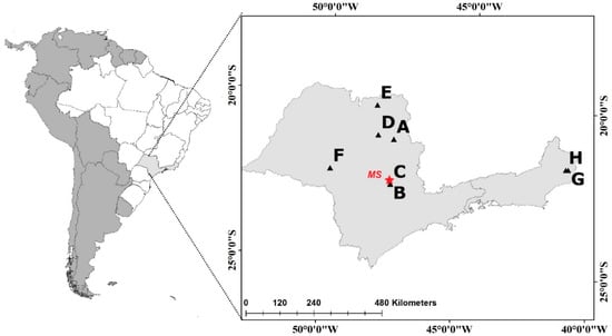
Figure 1.
Geographical position of sampled soils (A to H) and the University of São Paulo weather station (MS) in Piracicaba (SP), Brazil.

Table 1.
Hydraulic parameters of the soils according to the Van Genuchten equation.
Daily meteorological data were obtained for a 38-year period (1978–2017) from the University of São Paulo weather station in Piracicaba, Brazil (22.703° S; 47.624° W, Figure 1), representing the sub-tropical winter-dry climate (Koeppen Cwa) of southeast Brazil. Potential (reference) evapotranspiration for a hypothetical grass surface was calculated based on the Penman–Monteith (ET0P, mm d−1) Equation (1) [24]:
or, in cases where wind speed was unavailable, using the Hargreaves (ET0H, mm d−1) equation:
In (1) and (2), Rn and Rs are the net radiation at the crop surface and solar radiation (MJ m−2 d−1); G represents the soil heat flux density, which is usually ignored in daily calculations (MJ m−2 d−1); T (°C) and u2 (m s−1) are mean temperature and wind speed at 2 m height, respectively; (es − ea) is the vapor pressure deficit (kPa); Δ is the slope of the vapor pressure curve (kPa °C−1); and γ is the psychometric constant, equal to 0.06317 kPa °C−1 for the Piracicaba weather station.
2.3. HYDRUS-1D Numerical Modelling
The HYDRUS-1D model numerically simulates the temporal and spatial changes in water content by the Richards equation:
In this equation, θ is soil water content (cm3 cm−3), t is time (s), z is the vertical space coordinate (cm), k is the hydraulic conductivity (cm s−1), h represents pressure head (cm), and S is the sink term (s−1) accounting for the volume of water removed from the soil per unit of time due to crop water uptake and described by
where Sp is the potential water uptake rate (s−1) calculated from the potential transpiration rate Tp (cms−1) distributed over the root zone based on the normalized root density distribution function β(z,t) (cm−1). 0 ≤ α(h) ≤ 1 is a dimensionless root water uptake stress reduction function proposed by Feddes et al. (1978), defined by crop dependent parameters described for grass in [25]. Tp is calculated by
where k is an extinction coefficient usually within the range between 0.5–0.75.
The atmospheric boundary condition at the top of the soil surface is supplied to HYDRUS-1D by the daily variable potential evaporation Ep(t) (6) and precipitation P, besides a minimum and maximum allowed pressure head at the soil surface (hCritA and hS).
A unit vertical hydraulic gradient or free drainage boundary condition was implemented for the lower boundary of the 100 cm soil profile, as the groundwater level is very deep in these soils. For all scenarios, the initial condition was set to −100 cm pressure head in the entire profile. Temporal and spatial discretization for finite element method of HYDRUS-1D varied significantly to reach the lowest possible water balance error by the end of each simulation for each soil profile.
Simulations were performed for two standard conditions: bare soil (BS; no crop, no transpiration) and for grass-covered soil (G). One real set of weather data for 38 years and six generated ones by LARS-WG for 50 years were used for the top boundary conditions. As reference crop, we simulated grass with a leaf area index (LAI) equal to 2.88 [24] and with three different rooting depths (30, 60, or 90 cm), referred to as G30, G60, and G90 scenarios. Accordingly, four cropping/rooting scenarios (BS, G30, G60, G90) together with eight soils and seven weather data sets resulted in 224 different scenarios.
2.4. Soil Drainability Index
An a priori prediction of drainage throughout soil profile properties would be a useful tool for irrigation and fertilization management, but without experimentation or numerical modelling this is not an easy task, especially in nonuniform layered soils. In the drainage process, each soil layer has its own specific impact on water transmission to the bottom of the profile. There are many factors that could be considered to examine the effect of each layer on the overall drainability, summarized in their hydraulic properties, such as saturated and unsaturated hydraulic conductivity and corresponding water contents. Additionally, the thickness of each layer is effective as it represents the flow domain. Consequently, a conceptual indicator could be defined under some assumptions that would correspond to overall drainability of a soil. It would give a general idea about to what extent leaching occurs under bare soil condition. We call this indicator the soil drainability index (SDI).
Considering a soil with n layers, each with a thickness Li (L) and a water content θi (L3 L−3), it is reasonable to assume that maximum water storage (θs,iLi) is related to drainability. Furthermore, the water conducting properties of the layers will affect the rate at which drainage occurs. Hydraulic conductivity K may vary by orders of magnitude between soil layers, and the relative hydraulic conductivity (K/Ksat) seems a more plausible alternative. Then, drainability might be correlated to the sum of products of water storage and relative K for all soil layers. To test this hypothesis, we considered the soil profile at near saturation (ns in parameter subscripts) with a static value of pressure head to be evaluated at values of −1 or −3 cm. These small tensions can remove the effect of macropore flow to a great extent, especially as saturated hydraulic conductivity measurements were performed on undisturbed samples. In order not to make the drainability increase with increasing soil depth, the total sum of values was divided by the total depth, resulting in the following expression for the dimensionless soil drainability index (SDI):
2.5. Supervised Machine Learning
Supervised machine learning aims to map an input to an output based on an example of input–output pairs, including process uncertainty. Simulation of drainage in 8 soils combined to 7 weather scenarios and 4 cropping scenarios (BS, G30, 60, and 90) will result in 2688 number of monthly drainage values. Considering drainage related to reference evapotranspiration in bare soil and to transpiration in the grass scenarios, precipitation, and the SDI of the soil, then the monthly drainage rate could be predicted through machine learning methods. For this purpose, parametric techniques, including the linear model (LM) and stepwise linear model (SWLM), in addition to nonparametric methods, such as support vector machines (SVMs), Gaussian process regression (GPR), and the ensemble method (ENS), are utilized.
Parametric supervised machine learning optimizes the parameters of an a priori known learning function (f(.)) in (8) to achieve the best fit to data by minimizing the sum of squared errors (SSE).
where is the coefficient vector of parameters to be estimated, is the transpose of the variable vector for k variables, and ε is the error, with zero mean, normally and independently distributed with constant variance of σ2. f(.), or the learning function is an a priori specified model in parametric supervised methods [20].
In nonparametric regression, any number of latent functions f(.) in (8) for each pair of data can be generated and left unspecified, but these functions should be smooth and flexible. It means a particular subset of random latent functions f = {f1, …, fn} corresponds to input f = {X1, …, Xn}. In Gaussian process regressions, it is a priori assumed that all f(.) own a normal distribution looking like f(X) ~ GP(,cov(f)), where is the mean and cov(f) is covariance or kernel function.
Therefore, proper selection of kernel or covariance function is an important task since they determine the sample properties, such as smoothness, length scale, and amplitude, which are drawn from the GP to give a precise prediction for responses with inputs, which are close to trained data points in training stage. For example, Equation (9) is a squared exponential kernel function which is used in this study for GPR named GPR-SE.
where amplitude σf and the characteristic length scale σl are kernel (hyper) parameters.
A support vector machine (SVM) also maps output from a labelled training input–output dataset. The input data through kernel functions are projected into a higher dimensional space, called feature space, to find the output (y = f(x,w) + noise) via f(x,w) = w.φ(Xi) + b, where φ(Xi) is the projected input data into feature space, and w and b are weight vector parameter and bias of the searched regression function, respectively. The support vector regression function can be obtained as:
These Lagrange multipliers (α and α*) are support vectors and different Gaussian, linear, and second order polynomial kernel functions , , were selected, too, for SVMs.
Algorithms such as bootstrap aggregation (Bagging), proposed by [26], or least squares boosting (LSboost) are the most commonly used techniques for ensemble learning regressions. Regression ensembles include many weak learners that predict the output via two algorithms, Bagging or LSboost, called ENS-B and ENS-L. A detailed explanation regarding machine learning methods used in this study can be found in [20].
To examine the effect of SDI on simulation of monthly drainage, two scenarios including predictors, with SDI and without SDI (SDI, no SDI), were performed under the seven weather scenarios by machine learning algorithms. A total of 70% of data were randomly chosen for training the model and the remaining unseen data verified the MLTs in the testing stage.
3. Results
3.1. Climatic Data and Calibration of LARS-WG
As wind speed is not a generated weather data by LARS-WG, using the Penman–Monteith Equation (1) for prediction of ET0P was not feasible, and Equation (2) was used instead to predict ET0H. However, without calibration of this equation, on average, ET0H is 7.95% ± 3.75% larger than the ET0P except in August, September, and October, when it is about 1.8% smaller. After calibration, the coefficient in Equation (2) was needed to change to 0.01266, where ET0H was only 2.9% ± 2.04% greater than ET0P for the first half of year and for the second half of year ET0P was 5.10% ± 3.52% is larger than ET0H, as shown in Figure 2a. In general, the RMSE between ET0H and ET0P reduced from 0.60 to 0.54 mm d−1 after calibration. Figure 2b also provided the observed values of monthly maximum and minimum temperature and solar radiation from 38 years of measured data.
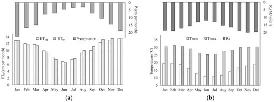
Figure 2.
Average monthly reference evapotranspiration (ET0) predicted by the calibrated Hargraves equation (ET0H) and the Penman–Monteith equation (ET0P), precipitation (P) (a); and maximum and minimum temperature (Tmax and Tmin) and solar radiation (Rs) (b) for the University of São Paulo weather station in Piracicaba (SP), Brazil.
For calibration of LARS-WG, observed data from 1978–2015 were compared to simulated data by LARS-WG through a baseline climate scenario. Monthly values of rainfall and reference evapotranspiration calculated using the Hargraves Equation (2), as well as average temperature and solar radiation are simulated closely to observed values with R2 more than 98% for all cases (Figure 3).
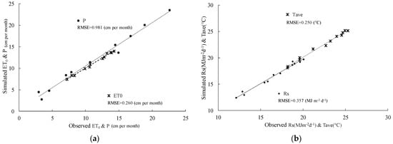
Figure 3.
Observed meteorological data versus simulated ones by LARS-WG: (a) Rainfall (P) and evapotranspiration (ET0); (b): radiation (Ra) and average temperature (Tave).
In order to determine if the seasonal wet/dry series and the meteorological variables had a high probability of belonging to the same distribution as the observed data, the calibration was also verified by the Kolmogorov–Smirnov (K-S) test close to 0 and p-values close to 1 for all cases (data not shown). For the assessment of drainage or plant water availability studies, the concept of wet and dry spell length (WSL or DSL) in weather data played an important role. WSL and DSL were well simulated with high correlations (Figure 4), showing an excellent ability in proper weather data generation.
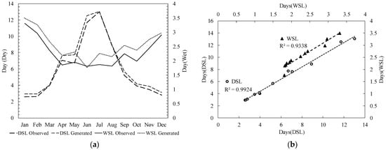
Figure 4.
Monthly observed and generated dry and wet spell length (DSL and WSL) (a); and correlation of observed and generated DSL and WSL (b).
3.2. Simulations with the Bare Soil Scenario
Figure 5 showed monthly drainage and evaporation with respective standard deviation versus rainfall evaluated from bare soil (BS) simulations, using the 38 years of meteorological data for all eight soils (A to H). Higher drainage occurs in the rainy months, October to March. Monthly average of rainfall (10.6 ± 6 cm) showed larger standard deviation in drier than in rainy months. This was attributed to drainage and evaporation in bare soil, with standard deviations of about 10% to 20% of the average value in rainy months versus 20% to 30% in dry months (Figure 5).
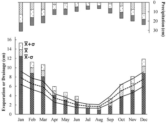
Figure 5.
Monthly drainage, evaporation, and rainfall averages and standard deviations for all soils under the bare soil (BS) scenario.
Regarding soil types, Figure 6 showed the SDI of each soil profile (A–H) calculated by Equation (7), assuming two different pressure head criteria, −1 and −3 cm. Resulting values were plotted against the average annual drainage predicted from respective bare soil profiles by the Hydrus simulations. The average annual precipitation for this 38-year series of weather data resulted in very close or more than 80 cm per year of drainage in bare soils E, G, A, and B, decreasing to just above 55 cm in soil C. Standard deviations among years were close to 20 cm for all soils. This allowed for the conclusion that under this climate, differences in soil hydraulic properties among soils may lead to a variation in bare soil drainage partitioning of the order of 40% to 70% of the average annual rainfall.
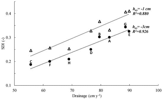
Figure 6.
Soil drainage index (SDI) of each soil (A to H), calculated using hns = −1 cm or hns = −3 cm versus the average annual drainage under the bare soil (BS) scenario.
Furthermore, Figure 6 showed an excellent correlation between SDI and annual drainage for both values of hns, with R2 around 0.9. This small change near saturation matric potential is usually associated with a great difference in hydraulic conductivity, while considering hns equal to zero matric potential (h0 = hs) results in a very weak correlation (R2 = 0.42) between SDI and annual drainage. This confirmed a good performance of SDI as a predictor of annual drainage, even though, for soils with lower SDI, around 0.2, there was a less strong correlation. Considering hns = −3 cm, the correlation coefficient is slightly higher than for hns = −1 cm (0.93 versus 0.88). Therefore, this near saturation-based index seems a good indicator of drainability, requiring the knowledge of water content at a fixed pressure head and the corresponding relative hydraulic conductivity.
From Figure 7 it is obvious that all the machine learning-based models performed better when SDI is used among predictors. It can be inferred that including SDI in the model was less effective for SVM-L and SVM-P, showing a drop of 17% and 18% in RMSE, respectively, and an increase of about 4% in R2 compared to the simulations with the same algorithms but without SDI.
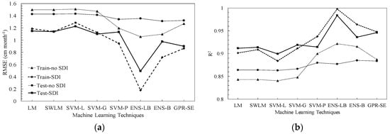
Figure 7.
Performance of proposed models including RMSE (a) and R2 (b) for prediction of bare soil drainage. (LM: linear model, SLM: stepwise linear mode, SVM-L, G & P: support vector machine with linear, Gaussian and polynomial kernel function, ENS-L&B: ensemble with LS boosting and Bagging algorithms, GPR-SE: Gaussian process regression with squared exponential kernel function).
The equations for prediction of monthly drainage prediction (D) using LM and SWLM were brought for both SDI and no-SDI scenarios, as , , , and . There was no interaction between ET0 and P which made the obtained equation in order to predict monthly drainage for SWLM to be the same as for LM in no-SDI scenarios. However, introducing SDI formed interactions with P and ET0 to improve the model performance, as this better performance was also clear in Figure 7, where RMSE lessened from 1.427 for Equation (11) to 1.148 and 1.137 cm month−1 for (12) and (13), respectively. These Equations (11)–(13) are as follows:
Ensemble regression ENS-LB gave the best fit in SDI and no SDI scenarios. In the model with SDI as the third predictor, R2 of 0.983 and an RMSE of 0.492 cm month−1 are obtained in the testing stage, which means prediction of drainage is much more reliable in drier months with monthly drainage between 2 to 5 cm. This was expected, since the incorporation of weak learners in an ensemble method makes estimations less likely to be biased [27].
Considering bagging and boosting algorithms in this study which are based on decision tree learners, the SDI parameter could enhance the decision-making capability of the ensemble model, especially when there was a strong relation between drainage and SDI, as shown in Figure 6. Superiority of ENS-LB compared to ENS-B was due to the fact that, at every step, the ensemble fitted a new learner to the difference between the observed drainage and the aggregated prediction of all learners grown previously. Among kernel-based algorithms, including SVMs and GPR, the latter showed better results with an R2 of 0.946 and RMSE of 0.899 cm month−1 for the model with SDI. However, in no-SDI, this accuracy decreased by 0.062 in R2 and 0.421 cm month−1 in RMSE. SVM-G with an RMSE of 1.100 cm month−1 was slightly better than other SVMs for prediction of annual drainage, again where SDI was considered as an input.
3.3. Simulations with Grass-Covered Lands (Pasture)
The presence of a vegetation covers reduced bottom drainage due to root water uptake, but the intensity of this drainage reduction dependent on the hydraulic properties of soil layers and rooting depth and distribution. To illustrate this, Figure 8 showed monthly average drainage and evapotranspiration from soils covered with grass with three rooting depths (30, 60, and 90 cm; scenarios G30, G60, and G90) together with the values (drainage and evaporation) for BS. Comparing BS to the grass scenarios, monthly drainage was reduced by 30% to 50% with G30, G60, and G90 scenarios.
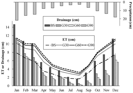
Figure 8.
Monthly average of drainage and evapotranspiration using real climatic data for eight soils under BS (bare soil), G30, G60, and G90 (Grass with 30, 60 and 90 cm rooting depth) scenarios.
Figure 8 also gave the details and comparisons of evapotranspiration (ET) due to climatic conditions under all grass types simulations and evaporation from bare soil. ET increased from G30 to G60 to G90, but the increase between G30 and G60 was higher than between G60 and G90. This showed that increasing rooting depth beyond a certain depth lead to a very modest increase in transpiration, as also confirmed by the data in Table 2. This depth then corresponded to an available water content capable of maintaining potential transpiration for most of the occurring weather conditions.
Table 2.
Monthly averages (and, between brackets, standard deviations) of actual transpiration (Ta), drainage (D), and evaporation (Ev), all in cm month−1, for G30, G60, and G90 scenarios in the wet (October to March) and dry seasons (April to September).
Seasonally speaking, actual transpiration in rainy months was just above twice that of dry months because of the higher amount of available water in the root zone. Averaging between G30, G60, and G90, 5.6 (±2.4) cm month−1 of transpiration results from 7.7 (±0.9) cm (corresponding to 68% of total Ta) transpiration in rainy months and 3.6 (±1.1) cm (32%) in the dry months, from April to September. The seasonal dependency of transpiration demonstrated the typical response to atmospheric demand and soil moisture supply on grass. Higher rainfall amounts returned to the atmosphere at maximum rates by evapotranspiration. In dry months with a higher vapor pressure deficit, atmospheric demand increased but transpiration was less due to limiting soil water supply.
Overall, predicted evapotranspiration for these scenarios ranged from 761 and 844 to 886 mm y−1 (standard deviations around 35 mm y−1) for G30, G60, and G90. The observed reduction of evapotranspiration when rooting depth is shallower allows one to understand the effect of conversion of deeply rooted crops to shallow rooted ones or land cover change as results, for example, from deforestation.
The ratio of actual to potential ET for different grass scenarios as in Figure 9 showed that rainfed crops were under frequent drought stress, even in the wetter months, and irrigation could improve crop yield and, subsequently, water use efficiency. The use of a fixed and constant LAI of 2.88 resulted in equal potential evapotranspiration predictions for G30, G60, and G90, and increasing the rooting depth from 30 to 60 cm allowed increasing ETa by about 10%. In the case of endoalic soils, common in Precambrian surfaces under a tropical humid climate, an increase of rooting depth can be sometimes accomplished by increasing soil pH using chalk, thus decreasing soluble aluminum contents.
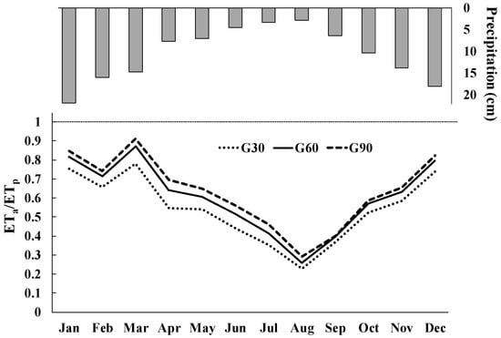
Figure 9.
Ratio of actual to potential evapotranspiration for three grass scenarios; average monthly values from all soils.
Similar to the procedure for the prediction of drainage from a bare soil profile, drainage prediction from grass covered lands (G30, G60, and G90) was performed by machine learning methods, replacing ET0 by the actual transpiration of grass (Tp), obtained by simulation with the Richards equation under different atmospheric boundary conditions. The values of RMSE and R2 for all algorithms were shown in Figure 10. In the bare soil scenario, there was no trace of soil effect if SDI was not considered and the system would be only plant atmosphere; however, in the grass-based scenarios, Hydrus obtains plant transpiration through numerical simulation, recalling Equation (5), where the hydraulic parameters of the soil affected the value of Tp in different times and different soils. In this way, SDI addition can be the soil representative in the grass scenario besides Tp and the system even without SDI is soil–plant–atmosphere. Therefore, for machine learning methods, the introduction of SDI to predict drainage for grass-based scenarios should not be the same as it was for bare soil.
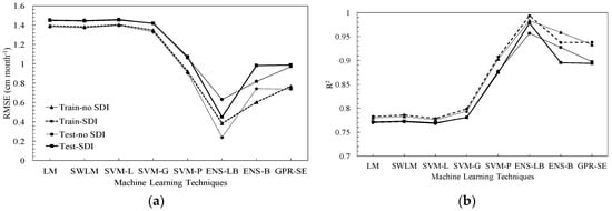
Figure 10.
Performance of proposed models including RMSE (a) and R2 (b) for prediction of grass-covered soil drainage.
Plant participation intensively affected the accuracy of parametric models, where RMSE of LM and SWLM on testing data increased by 20.7% and 21.21% in the model with SDI. These models were shown in Equations (14), (15), (16), and (17), respectively, for models with and without SDI.
As already mentioned, SDI engagement in the model did not make a significant difference in better prediction of drainage, as was clear from the comparison of Figure 7 and Figure 10, except for ENS-BL. For this algorithm, RMSE of predicted and observed values for the testing dataset decreased from 0.629 to 0.448 cm month−1.
4. Discussion
In the present work a new index to approximate annual drainage from a layered soil under no cropping was proposed. To the best of our knowledge there is no study focusing on simple methods to estimate drainage in tropical soils and only a few studies are available for measurement of drainage flux. The main hypothesis was to relate the drainage under atmospheric boundary conditions with hydraulic properties of the soil. This link was made by the soil drainabilty index (SDI) composed of near saturated (e.g., at −1 and −3 cm) and saturated hydraulic conductivities beside saturated water content of every single layer. The index requires fewer parameters to estimate annual drainage compared to typical modelling and experimental methods. However, the SDI concept needs more verification through experimental data, not easily available for most scenarios.
We found that any prediction of rainfall dependent problems will be less precise in the drier months. The eight analyzed soil types drained 56.5% (±9%) of monthly rainfall if left bare, whereas the remaining portion of the water budget was lost via evaporation. Thus, 40% to 70% of the average annual rainfall could be lost due to bottom drainage from bare soils, similar to the results reported in [28], where drainage could be 35% of precipitation in bare soils with a clayey texture. In a modelling study [29], authors showed 65% of precipitation during 1961–1990 to be drained from a bare Cambisol as well.
Deep drainage may be a water saving measure in groundwater irrigation; nevertheless, it accounts for non-productive loss of water in deep groundwater scenarios, common in most soils in Brazil. Under these conditions, higher drainage results in lower transpiration and reduced biomass production. Intensive fertilization may pose a serious risk of groundwater contamination because of drainage and leaching.
Moreover, having a single soil hydraulic related parameter, such as SDI, representing the soil profile’s role in water flow, could be used as a single predictor, besides atmospheric and plant related parameters, to predict fluxes such as drainage. SDI engagement ameliorated the performance of parametric machine learning models (linear and stepwise models) by about 20% in terms of RMSE; though RMSE of 0.492 cm month−1 proved the robust method of ensemble for prediction of drainage with SDI.
Simulated bottom drainage for grass-covered scenarios with rooting depths of 30, 60, and 90 cm was 501 ± 40.3, 420 ± 31.5, and 382 ± 30.8 mm y−1, respectively, within the range between 145–703 mm y−1 reported for recharge rate data in grass cultivated lands in [29]. Referring to land use change in Brazil, one could consider the effect of a change from native vegetation with more than 90 cm root depth, such as the savannah, to a shallower rooted grass for grazing purposes, resulting in a 25% increase in drainage and a more non-productive loss of water according to our simulations. There is, on average, a 40% reduction in monthly drainage due to plantation.
Comparing the simulated ET of 3.2 ± 0.4 mm d−1 for rainy months and 1.4 ± 0.45 mm d−1 for dry months for all grass covered scenarios, regardless of root depth, to measured values, good agreement is found. Using remote sensing techniques, Andrade et al. (2014) [30] measured evapotranspiration in grass cover areas of Brazil to be less than 1.5 mm d−1 between May and October. Feltrin et al., (2017) [31] used lysimeters and recorded 2.95 mm d−1 of evapotranspiration in a grass covered location in Rio Grande do Sul State, Brazil. The value of 2.25–2.43 mm d−1 was reported from a macroscale analysis for Mato Grosso State, Brazil [32].
Considering a leaf area index (LAI) between 0.4 and 1.1 resulted in a measured ET of 2.6 ± 0.9 mm d−1 for grass cultivated in the cerrado biome of central Brazil [33]. However, a LAI of 3.2 (close to our assumption of LAI 2.88) for an ungrazed Brachiaria pasture in central Brazil increased calculated ET to 3.4 mm d−1 [34]. A high infiltration rate of very sandy soils with grass cultivation in the study by Nóbrega et al., (2017) [35] resulted in 1.19 ± 0.52 mm d−1 and 2.15 ± 0.58 mm d−1 evapotranspiration in the cerrado. The reported value of evapotranspiration for wet months in our study is within the comprehensive finding of 3–4 mm d−1, as reported in [36], for grass cultivation in a tropical condition. We did not observe significant improvement in prediction of drainage by incorporation of the SDI factor in machine learning models, although it was expected because the Tp factor carries the role of soil profile behavior, hence SDI does not seem to be influential.
5. Conclusions
A soil drainability index (SDI) is defined in order to predict the annual drainage from bare soils and grass cultivated soil. Fewer parameters are required to estimate annual drainage based on SDI compared to typical modelling and experimental methods. When SDI is used as a predictor for monthly drainage from bare soils using machine-learning models, performance of these models improved significantly. The introduction of SDI for drainage prediction from planted soils enhanced the robustness of models, but less than bare soil. Among machine learning methods, ensemble regression with least squares boosting aggregation algorithm predicted monthly drainage better than Gaussian process regression and support vector machines. The RMSE values for testing data in bare soil scenarios were low, around 1.2 cm month−1. In grass-cropped scenarios, the accuracy of the models was lower, with RMSE up to about 1.5 cm month−1, probably due to errors associated to the prediction of actual crop transpiration.
Author Contributions
Conceptualization, A.M.K. and Q.d.J.v.L.; methodology, A.M.K, Q.d.J.v.L; formal analysis, A.M.K.; writing—original draft preparation, A.M.K.; writing—review and editing, A.M.K, Q.d.J.v.L. and B.V.I.; supervision, Q.d.J.v.L. and B.V.I.
Funding
The first author is grateful to FAPESP (Fundação de Amparo à Pesquisa do Estado de São Paulo) foundation, Brazil, for providing financial support (scholarship) for his study (process number 2016/18636-7).
Conflicts of Interest
The authors declare no conflict of interest.
References
- FAO. How to Feed the World in 2050; FAO: Rome, Italy, 2009. [Google Scholar]
- Jägermeyr, J.; Gerten, D.; Heinke, J.; Schaphoff, S.; Kummu, M.; Lucht, W. Water savings potentials of irrigation systems: Global simulation of processes and linkages. Hydrol. Earth Syst. Sci. 2015, 19, 3073–3091. [Google Scholar] [CrossRef]
- Sentelhas, P.C.; Battisti, R.; Câmara, G.M.S.; Farias, J.R.B.; Hampf, A.C.; Nendel, C. The soybean yield gap in Brazil-magnitude, causes and possible solutions for sustainable production. J. Agric. Sci. 2015, 153, 1394–1411. [Google Scholar] [CrossRef]
- Wu, C.L.; Shukla, S.; Shrestha, N.K. Evapotranspiration from drained wetlands with different hydrologic regimes: Drivers, modeling, and storage functions. J. Hydrol. 2016, 538, 416–428. [Google Scholar] [CrossRef]
- Šimůnek, J.; van Genuchten, M.T.; Šejna, M. Recent Developments and Applications of the HYDRUS Computer Software Packages. Vadose Zone J. 2016, 15, 1–25. [Google Scholar] [CrossRef]
- Chen, M.; Willgoose, G.R.; Saco, P.M. Spatial prediction of temporal soil moisture dynamics using HYDRUS-1D. Hydrol. Process. 2014, 28, 171–185. [Google Scholar] [CrossRef]
- Liu, T.; Lai, J.; Luo, Y.; Liu, L. Study on extinction depth and steady water storage in root zone based on lysimeter experiment and HYDRUS-1D simulation. Hydrol. Res. 2015, 46, 871–879. [Google Scholar] [CrossRef]
- Leterme, B.; Mallants, D.; Jacques, D. Sensitivity of groundwater recharge using climatic analogues and HYDRUS-1D. Hydrol. Earth Syst. Sci. 2012, 16, 2485–2497. [Google Scholar] [CrossRef]
- Ries, F.; Lange, J.; Schmidt, S.; Puhlmann, H.; Sauter, M. Recharge estimation and soil moisture dynamics in a Mediterranean, semi-arid karst region. Hydrol. Earth Syst. Sci. 2015, 19, 1439–1456. [Google Scholar] [CrossRef]
- Patle, G.T.; Singh, D.K.; Sarangi, A.; Sahoo, R.N. Modelling of groundwater recharge potential from irrigated paddy field under changing climate. Paddy Water Environ. 2017, 15, 413–423. [Google Scholar] [CrossRef]
- Zhu, Y.; Ren, L.; Zhang, Q.; Yu, Z.; Wu, Y.; Feng, H. The contribution of groundwater to soil moisture in Populus euphratica root zone layer. In Ecohydrology of Surface and Groundwater Dependent Systems: Concepts, Methods and Recent Developments. Proceedings of Symposium JS. 1 at the Joint Convention of the International Association of Hydrological Sciences (IAHS) and the International Association; IAHS Press: Hyderabad, India, 2009; pp. 181–190. [Google Scholar]
- Shouse, P.J.; Ayars, J.E.; ŠimŮnek, J. Simulating root water uptake from a shallow saline groundwater resource. Agric. Water Manag. 2011, 98, 784–790. [Google Scholar] [CrossRef]
- Zhu, Y.; Ren, L.; Horton, R.; Lü, H.; Chen, X.; Jia, Y.; Wang, Z.; Sudicky, E.A. Estimating the contribution of groundwater to rootzone soil moisture. Hydrol. Res. 2013, 44, 1102–1113. [Google Scholar] [CrossRef]
- Hou, L.; Zhou, Y.; Bao, H.; Wenninger, J. Simulation of maize (Zea mays L.) water use with the HYDRUS-1D model in the semi-arid Hailiutu River catchment, Northwest China. Hydrol. Sci. J. 2017, 62, 93–103. [Google Scholar]
- Zhao, Y.; Si, B.; He, H.; Xu, J.; Peth, S.; Horn, R. Modeling of Coupled Water and Heat Transfer in Freezing and Thawing Soils, Inner Mongolia. Water 2016, 8, 424. [Google Scholar] [CrossRef]
- Yang, R.; Tong, J.; Hu, B.X.; Li, J.; Wei, W. Simulating water and nitrogen loss from an irrigated paddy field under continuously flooded condition with Hydrus-1D model. Environ. Sci. Pollut. Res. 2017, 24, 15089–15106. [Google Scholar] [CrossRef]
- He, K.; Yang, Y.; Yang, Y.; Chen, S.; Hu, Q.; Liu, X.; Gao, F. HYDRUS Simulation of Sustainable Brackish Water Irrigation in a Winter Wheat-Summer Maize Rotation System in the North China Plain. Water 2017, 9, 536. [Google Scholar] [CrossRef]
- Lamorski, K.; Pachepsky, Y.; Sławiński, C.; Walczak, R.T. Using support vector machines to develop pedotransfer functions for water retention of soils in Poland. Soil Sci. Soc. Am. J. 2008, 72, 1243–1247. [Google Scholar] [CrossRef]
- Elbisy, M.S. Support Vector Machine and regression analysis to predict the field hydraulic conductivity of sandy soil. KSCE J. Civ. Eng. 2015, 19, 2307–2316. [Google Scholar] [CrossRef]
- Kotlar, A.M.; Iversen, B.V.; de Jong van Lier, Q. Evaluation of Parametric and Nonparametric Machine-Learning Techniques for Prediction of Saturated and Near-Saturated Hydraulic Conductivity. Vadose Zone J. 2019, 18. [Google Scholar] [CrossRef]
- Semenov, M.A.; Barrow, E.M.; Lars-Wg, A. A Stochastic Weather Generator for Use in Climate Impact Studies; User Man Herts UK: Rothamsted Research, UK, 2002. [Google Scholar]
- De Jong van Lier, Q. Field capacity, a valid upper limit of crop available water? Agric. Water Manag. 2017, 193, 214–220. [Google Scholar] [CrossRef]
- Van Genuchten, M.T. A closed-form equation for predicting the hydraulic conductivity of unsaturated soils. Soil Sci. Soc. Am. J. 1980, 44, 892–898. [Google Scholar] [CrossRef]
- Allen, R.G.; Pereira, L.S.; Raes, D.; Smith, M. Crop Evapotranspiration-Guidelines for Computing Crop Water Requirements-FAO Irrigation and Drainage Paper 56; FAO: Rome, Italy, 1998; Volume 300, p. D05109. [Google Scholar]
- Feddes, R.A.; Kowalik, P.J.; Zaradny, H. Simulation of Field Water Use and Crop Yield; Simulation Monographs: Wageningen, The Netherlands, 1978; Volume 2. [Google Scholar]
- Breiman, L. Bagging predictors. Mach. Learn. 1996, 24, 123–140. [Google Scholar] [CrossRef]
- Møller, A.B.; Beucher, A.; Iversen, B.V.; Greve, M.H. Predicting artificially drained areas by means of a selective model ensemble. Geoderma 2018, 320, 30–42. [Google Scholar] [CrossRef]
- De Faria, R.T.; Bowen, W.T. Evaluation of DSSAT soil-water balance module under cropped and bare soil conditions. Braz. Arch. Biol. Technol. 2003, 46, 489–498. [Google Scholar] [CrossRef]
- Oliveira, P.T.S.; Wendland, E.; Nearing, M.A.; Scott, R.L.; Rosolem, R.; da Rocha, H.R. The water balance components of undisturbed tropical woodlands in the Brazilian cerrado. Hydrol. Earth Syst. Sci. 2015, 19, 2899–2910. [Google Scholar] [CrossRef]
- Andrade, R.G.; de Teixeiraa, A.H.C.; Sanob, E.E.; Leivasa, J.F. Pasture evapotranspiration as indicators of degradation in the Brazilian Savanna. A case study for Alto Tocantins watershed. In Proceedings Volume 9239, Remote Sensing for Agriculture, Ecosystems, and Hydrology XVI; SPIE REMOTE SENSING: Amsterdam, The Netherlands, 2014; Volume 2014, p. 92391Z-1. [Google Scholar]
- Feltrin, R.M.; de Paiva, J.B.D.; de Paiva, E.M.C.D.; Meissner, R.; Rupp, H.; Borg, H. Use of Lysimeters to Assess Water Balance Components in Grassland and Atlantic Forest in Southern Brazil. Water Air Soil Pollut. 2017, 228, 247. [Google Scholar] [CrossRef]
- Lathuillière, M.J.; Johnson, M.S.; Donner, S.D. Water use by terrestrial ecosystems: Temporal variability in rainforest and agricultural contributions to evapotranspiration in Mato Grosso, Brazil. Environ. Res. Lett. 2012, 7, 24024. [Google Scholar] [CrossRef]
- Meirelles, M.L.; Franco, A.C.; Farias, S.E.M.; Bracho, R. Evapotranspiration and plant–atmospheric coupling in a Brachiaria brizantha pasture in the Brazilian savannah region. Grass Forage Sci. 2011, 66, 206–213. [Google Scholar] [CrossRef]
- Santos, A.J.B.; Quesada, C.A.; Da Silva, G.T.; Maia, J.F.; Miranda, H.S.; Carlos Miranda, A.; Lloyd, J. High rates of net ecosystem carbon assimilation by Brachiara pasture in the Brazilian Cerrado. Glob. Chang. Biol. 2004, 10, 877–885. [Google Scholar] [CrossRef]
- Nóbrega, R.L.B.; Guzha, A.C.; Torres, G.N.; Kovacs, K.; Lamparter, G.; Amorim, R.S.S.; Couto, E.; Gerold, G. Effects of conversion of native cerrado vegetation to pasture on soil hydro-physical properties, evapotranspiration and streamflow on the Amazonian agricultural frontier. PLoS ONE 2017, 12, e0179414. [Google Scholar] [CrossRef]
- Sanches, L.; Vourlitis, G.L.; de Carvalho Alves, M.; Pinto-Júnior, O.B.; de Souza Nogueira, J. Seasonal patterns of evapotranspiration for a Vochysia divergens forest in the Brazilian Pantanal. Wetlands 2011, 31, 1215–1225. [Google Scholar] [CrossRef]
© 2019 by the authors. Licensee MDPI, Basel, Switzerland. This article is an open access article distributed under the terms and conditions of the Creative Commons Attribution (CC BY) license (http://creativecommons.org/licenses/by/4.0/).