A System Size Analysis of the Fireball Produced in Heavy-Ion Collisions ^†

Abstract

One of the main interests of high-energy physics is the study of the phase diagram and the localization of phase transitions from hadronic to quark–gluonic matter. There are different techniques to study the hot matter. One of them is femtoscopy, which uses two-particle correlations to extract spatiotemporal characteristics of the emission source. Another approach involves obtaining thermodynamic parameters from the momentum distributions of produced particles based on various theoretical models. In this research, we perform a comparative analysis of femtoscopic volumes and volumes obtained using the Tsallis statistical fit. This analysis allows us to estimate system size at the time of kinetic freeze-out and its dependence on collision centrality and energy. We observe that at high energies, the volume values estimated taking the two approaches diverge significantly, while at low energies, they are more consistent. In the future, these results can help to combine these two different methods and provide a more comprehensive picture of the fireball produced in heavy-ion collisions.

1. Introduction

Recently, a large amount of experimental data have been collected in high-energy physics for studying the properties of nuclear matter. One of the main interests is the study of phase transitions from regular hadronic matter to a deconfined state called quark–gluon plasma (QGP) [1,2,3,4]. This transition can occur at high temperatures and densities and can be shown on the Quantum ChromoDynamics (QCD) phase diagram in terms of temperature and baryonic chemical potential.

At low baryonic chemical potential, lattice calculations indicate the presence of a smooth transition—a crossover [5,6]. However, at higher chemical potential, lattice calculations are not possible, and effective models have to be used instead. These models suggest the presence of a first-order phase transition and the critical point separating it from the crossover.

QGP can be formed in ultrarelativistic heavy-ion collisions. After its formation, the hot matter expands and cools, which leads to the transition into the hadronic phase and reaches a state of statistical equilibrium until chemical freeze-out, when inelastic interactions between particles cease. Kinetic freeze-out occurs when hadrons stop interacting elastically, and their kinematic properties remain unchanged.

2. Materials and Methods

In our research, we use the published data from the STAR experiment obtained during the first stage of the Beam Energy Scan program at RHIC for Au+Au collisions at $\sqrt{s_{\mathrm{NN}}}=7.7,11.5,19.6,27$ and 39 GeV, aimed at localizing the phase transition boundary [7,8].

The main goal of this research is to estimate the size of the system formed in heavy-ion collisions using different methods and to compare the results obtained through different observables.

The first method is based on the application of a statistical model using Tsallis statistics [9,10,11]. The fireball is considered a thermodynamic system in the grand canonical ensemble (GCE), and thermodynamic characteristics, such as temperature and system volume, are extracted from the analysis of transverse momentum spectra.

The second method relies on femtoscopy. The interferometry method was initially proposed by Hanbury Brown and Twiss [12] in astrophysics and was later adapted for use in particle physics [13,14,15]. It has been applied in studies across a wide range of energies [16,17,18,19] to extract spatiotemporal properties of the homogeneity region at kinetic freeze-out by analyzing two-particle correlations of final particles.

2.1. Tsallis-3 Statistics

Tsallis entropy is defined as [9]

$$S=\sum _i{\displaystyle \frac{p_i^q-p_i}{1-q}},\sum _i{p}_i=1,$$

(1)

where $p_i$ is the probability of i-th microscopic state of the system and $q\in [0,\infty ]$ is the entropic parameter. In the Gibbs limit ($q\to 1$), the Tsallis entropy (1) recovers the Boltzmann–Gibbs entropy [9]:

$$S=\sum _i{p}_{i}ln{p}_i.$$

(2)

We can see that the Tsallis entropy generalizes the Boltzmann–Gibbs entropy, with the parameter q indicating the degree of deviation of a given generalized probability distribution from the Boltzmann–Gibbs one. There are a few variants of the Tsallis statistics [10].

In the Tsallis-3 statistics (Tsallis statistics with escort probabilities) [10,11] in the grand canonical ensemble, the thermodynamic potential $\Omega$ of the system can be written as

$$\Omega =\langle H\rangle -TS-\mu \langle N\rangle ,$$

(3)

where $\langle H\rangle ={\displaystyle \frac{1}{\theta }}{\sum }_i{p}_i^q{E}_i$ is the mean energy of the system, $\langle N\rangle ={\displaystyle \frac{1}{\theta }}{\sum }_i{p}_i^q{N}_i$ is the mean number of particles, and $\theta ={\sum }_i{p}_i^q$.

Let us consider a relativistic ideal gas in the Tsallis-3 statistics in the grand canonical ensemble with the Maxwell–Boltzmann statistics of particles. According to the principle of thermodynamic equilibrium for an open system, similar to the principle of maximum entropy for an isolated system, normalization expressions for the parameters $\Lambda =-\theta TS+\langle H\rangle -\mu \langle N\rangle$ and $\theta$ can be expressed as [11]

$$\left\{\begin{array}{c}{\displaystyle 1=\sum _{n=0}^{n_0}\frac{{\omega }^n}{n!\Gamma \left(\frac{1}{q-1}\right)}\underset{0}{\overset{\infty }{\int }}{t}^{\frac{2-q}{q-1}-n}{e}^{-t+{\beta }^{\prime }(\Lambda +\mu n)}{\left({\mathrm{K}}_2\left({\beta }^{\prime }m\right)\right)}^n\mathrm{d}t,}\hfill \\ {\displaystyle \theta =\sum _{n=0}^{n_0}\frac{{\omega }^n}{n!\Gamma \left(\frac{q}{q-1}\right)}\underset{0}{\overset{\infty }{\int }}{t}^{\frac{1}{q-1}-n}{e}^{-t+{\beta }^{\prime }(\Lambda +\mu n)}{\left({\mathrm{K}}_2\left({\beta }^{\prime }m\right)\right)}^n\mathrm{d}t,}\hfill \end{array}\right.$$

(4)

where ${\displaystyle \omega =\frac{gV}{2{\pi }^2}\frac{m^{2}T{\theta }^2}{q-1}}$, ${\beta }^{\prime }={\displaystyle \frac{-t(1-q)}{T{\theta }^2}}$ and $n_0$ is the number of terms of the series to be taken into account, starting from zero. The values of $\Lambda$ and $\theta$ are found by numerically solving the system of Equation (4). The expression for transverse momentum distribution in rapidity range $y\in [y_{min},y_{max}]$ takes the following form [11]:

$${\left.{\displaystyle \frac{{\mathrm{d}}^{2}N}{p_T\mathrm{d}{p}_T\mathrm{d}y}}\right|}_{y_{min}}^{y_{max}}={\displaystyle \frac{gV}{{\left(2\pi \right)}^2}}{m}_T\underset{y_{min}}{\overset{y_{max}}{\int }}\mathrm{d}ycoshy{\displaystyle \frac{1}{\theta }}\sum _{n=0}^{n_0}{\displaystyle \frac{{\omega }^n}{n!\Gamma \left(\frac{q}{q-1}\right)}}\underset{0}{\overset{\infty }{\int }}{t}^{{\displaystyle \frac{1}{q-1}}-n}{e}^{-t+{\beta }^{\prime }(\Lambda -m_{T}coshy+\mu (n+1))}{\left({\mathrm{K}}_2\left({\beta }^{\prime }m\right)\right)}^n\mathrm{d}t.$$

(5)

The fitting of the final particle spectra was performed using the ROOT analysis framework with MINUIT2 numerical minimization software library [20]. The technique of simultaneous fitting of all particle types by ${\chi }^2$-minimization method was applied, where parameters of the medium, such as temperature T and the parameter q, are common for all types of particles. The fitting procedure involves substituting some initial guess fit parameters (the state variables of GCE) into the system of Equation (4), which is then solved numerically to determine the values of the thermodynamic normalization functions $\Lambda$ and $\theta$. Calculated values of the normalization functions, along with the initial parameters, are then used in the final Formula (5)) for the transverse momentum distribution for ${\chi }^2$ minimization. The procedure can then be applied iteratively to reach the global minimum of fit parameters. For simultaneous fitting, we minimized the sum of ${\chi }^2$ for all particle species. Figure 1 shows the Tsallis-3 model fits for $K^{\pm },{\pi }^{\pm }$, at $\sqrt{s_{\mathrm{NN}}}$ = 7.7, 19.6, 39 GeV and centrality classes: 0–5%, 30–40%, 70–80%. The parameter values for all energies and centralities are presented in

Table A1. Tsallis-3 model fit of ${\pi }^{\pm }, K^{\pm }$ $p_T$-spectra at $\sqrt{s_{\mathrm{NN}}}$ = 7.7, 11.5, 19.6, 27, 39 GeV and centralities from 0–5%, to 70–80%. $p_T$ ranges: [0.5, 2], [0.25, 2] (GeV/c) are taken for ${\pi }^{\pm }$, $K^{\pm }$, correspondingly.

Centrality	T (MeV)	q	${\mathit{\chi }}^2$/NDF
7.7 GeV
0–5%	$187.5\pm 1.5$	$1.0221\pm 0.0022$	$131/61$
5–10%	$184.9\pm 1.7$	$1.0227\pm 0.0031$	$93/63$
10–20%	$186.9\pm 1.1$	$1.0346\pm 0.0034$	$67/63$
20–30%	$178.2\pm 1.0$	$1.0331\pm 0.0029$	$73/63$
30–40%	$170.5\pm 0.8$	$1.0277\pm 0.0030$	$70/62$
40–50%	$161.7\pm 0.9$	$1.0326\pm 0.0029$	$65/57$
50–60%	$151.6\pm 0.9$	$1.0206\pm 0.0031$	$81/57$
60–70%	$143.8\pm 1.0$	$1.0157\pm 0.0032$	$73/53$
70–80%	$136.8\pm 0.9$	$1.0082\pm 0.0041$	$66/44$
11.5 GeV
0–5%	$201.3\pm 1.7$	$1.0330\pm 0.0029$	$107/63$
5–10%	$197.6\pm 0.8$	$1.0316\pm 0.0007$	$75/65$
10–20%	$195.6\pm 1.1$	$1.0384\pm 0.0031$	$56/65$
20–30%	$190.8\pm 0.8$	$1.0412\pm 0.0028$	$41/65$
30–40%	$182.8\pm 1.0$	$1.0447\pm 0.0024$	$55/64$
40–50%	$173.0\pm 0.8$	$1.0363\pm 0.0020$	$62/64$
50–60%	$164.5\pm 0.9$	$1.0323\pm 0.0019$	$60/63$
60–70%	$154.9\pm 0.8$	$1.0228\pm 0.0023$	$82/56$
70–80%	$147.1\pm 0.9$	$1.0163\pm 0.0025$	$100/51$
19.6 GeV
0–5%	$218.9\pm 3.5$	$1.0479\pm 0.0010$	$75/67$
5–10%	$216.3\pm 2.3$	$1.0520\pm 0.0005$	$70/67$
10–20%	$210.1\pm 0.9$	$1.0502\pm 0.0025$	$57/67$
20–30%	$201.9\pm 1.0$	$1.0527\pm 0.0017$	$27/67$
30–40%	$191.6\pm 0.9$	$1.0443\pm 0.0019$	$49/67$
40–50%	$182.1\pm 0.8$	$1.0377\pm 0.0017$	$92/65$
50–60%	$174.0\pm 0.8$	$1.0343\pm 0.0016$	$159/65$
60–70%	$165.2\pm 0.8$	$1.0279\pm 0.0017$	$229/61$
70–80%	$154.6\pm 1.1$	$1.0219\pm 0.0020$	$177/58$
27 GeV
0–5%	$221.8\pm 1.9$	$1.0421\pm 0.0031$	$103/66$
5–10%	$221.2\pm 1.4$	$1.0465\pm 0.0004$	$76/67$
10–20%	$211.4\pm 0.1$	$1.0490\pm 0.0001$	$117/67$
20–30%	$209.5\pm 1.2$	$1.0570\pm 0.0022$	$32/67$
30–40%	$201.3\pm 0.0$	$1.0528\pm 0.0009$	$28/67$
40–50%	$191.3\pm 1.1$	$1.0486\pm 0.0016$	$49/67$
50–60%	$182.1\pm 0.9$	$1.0424\pm 0.0014$	$94/67$
60–70%	$172.5\pm 0.9$	$1.0351\pm 0.0014$	$180/67$
70–80%	$163.8\pm 0.9$	$1.0284\pm 0.0013$	$255/67$
39 GeV
0–5%	$232.6\pm 1.2$	$1.0454\pm 0.0007$	$86/67$
5–10%	$231.6\pm 1.3$	$1.0499\pm 0.0007$	$64/67$
10–20%	$229.1\pm 1.0$	$1.0568\pm 0.0007$	$42/67$
20–30%	$218.6\pm 0.3$	$1.0614\pm 0.0008$	$19/67$
30–40%	$205.0\pm 0.2$	$1.0612\pm 0.0012$	$28/67$
40–50%	$199.9\pm 1.2$	$1.0521\pm 0.0016$	$56/67$
50–60%	$185.0\pm 0.1$	$1.0493\pm 0.0010$	$134/67$
60–70%	$182.2\pm 1.1$	$1.0422\pm 0.0014$	$143/67$
70–80%	$174.9\pm 1.1$	$1.0354\pm 0.0015$	$216/67$

. The Tsallis-3 statistics are sensitive to the particle type; therefore, during the fitting process, protons were excluded, and only mesons were included in the fit. Since the next method uses combined data from ${\pi }^{+}$ and ${\pi }^{-}$, their spectra are also combined here. The low $p_T$ part of the pion spectra up to 0.5 GeV/c is affected by resonance decays and was excluded from the calculations. The fit ranges were [0.25, 2.00] GeV/c for kaons and [0.50, 2.00] GeV/c for pions. The volume values were obtained as a free fit parameter.

2.2. Femtoscopic Approach

The experimental correlation function is constructed using distributions of the relative pair momentum $\overrightarrow{q}=\overrightarrow{p_1}-\overrightarrow{p_2}$:

$$C\left(\overrightarrow{q}\right)={\displaystyle \frac{N\left(\overrightarrow{q}\right)}{D\left(\overrightarrow{q}\right)}},$$

(6)

where the numerator $N\left(\overrightarrow{q}\right)$ is constructed with pairs of particles from the same event and, thus, contains information on quantum statistics and effects of particle final state interactions [21], while the denominator $D\left(\overrightarrow{q}\right)$ uses uncorrelated pairs obtained from mix-events. The relative pair momentum $\overrightarrow{q}$, expressed in the longitudinal co-moving system (LCMS), is projected onto the Bertsch–Pratt coordinate system [22,23]. The $q_{out}$ component is directed along the pair transverse momentum $\overrightarrow{k_T}=({\overrightarrow{p}}_{T,1}+{\overrightarrow{p}}_{T,2})/2$, the $q_{long}$ component is directed along the beam axis, and the $q_{side}$ component is perpendicular to the other two directions. Further, the Bowler–Sinyukov Gaussian parametrization [24,25] is applied:

$$C\left(\overrightarrow{q}\right)\propto (1-\lambda )+K_{\mathrm{Coul}}\left(q_{\mathrm{inv}}\right)\lambda exp(-q_{\mathrm{o}}^2{R}_{\mathrm{o}}^2-q_{\mathrm{s}}^2{R}_{\mathrm{s}}^2-q_{\mathrm{l}}^2{R}_{\mathrm{l}}^2-2q_{\mathrm{o}}{q}_{\mathrm{s}}{R}_{\mathrm{os}}^2-2q_{\mathrm{o}}{q}_{\mathrm{l}}{R}_{\mathrm{ol}}^2),$$

(7)

where $K_{\mathrm{Coul}}\left(q_{\mathrm{inv}}\right)$ is the Coulomb correction factor, $\lambda$ is the correlation strength related to secondary particles from resonance decays, $R_{\mathrm{out},\mathrm{side},\mathrm{long}}$ are the correlation radii, and $R_{\mathrm{out}-\mathrm{side},\mathrm{out}-\mathrm{long}}$ are the cross terms. The particle emission source correlation radii are extracted by fitting. The radius $R_{\mathrm{side}}$ depends on the geometrical size of the source, $R_{\mathrm{out}}$ is influenced by both the geometrical size and the emission duration, and $R_{\mathrm{long}}$ depends on the system’s lifetime.

We use the data measured by the STAR collaboration during the BES-I program [8]. The dependence of the correlation radii on transverse mass, $m_T$, is considered below. The homogeneity region of the system is smaller for pairs with larger $m_T$ [26]. Therefore, to assess the entire volume of the system, we extrapolate the $m_T$-dependence of femtoscopic radii to the minimum possible transverse mass, $m_T=m$. We employed several parameterizations for this extrapolation: the first is grounded in basic hydrodynamic assumptions (known as $m_T$-scaling [27])

$$R_i\propto {\displaystyle \frac{1}{\sqrt{m_T}}},$$

(8)

the second uses a simple power-law model

$$R_i\propto m_T^{-\alpha },$$

(9)

and the third applies a model based on the Blast-Wave expansion scenario [28]

$$R_{\mathrm{side}}={\displaystyle \frac{R_0}{\sqrt{1+{\rho }_0^2(m/T+1/2)}}},R_{\mathrm{long}}=\tau \sqrt{{\displaystyle \frac{T}{m_T}}{\displaystyle \frac{{\mathrm{K}}_2(m_T/T)}{{\mathrm{K}}_2(m_T/T)}}},$$

(10)

where $i=\mathrm{out},\mathrm{side},\mathrm{long}$, ${\rho }_0$ is the maximum flow rapidity, and T is the kinetic freeze-out temperature. The values of these parameters are obtained by fitting ${\pi }^{\pm },K^{\pm },p,\overline{p}$ transverse momentum spectra using the Blast-Wave model [29] and are fixed for further analysis. These parameter values are listed in

Table A2. Blast-Wave model fit results for ${\pi }^{\pm }, K^{\pm }, p, \overline{p}$ $p_T$-spectra at $\sqrt{s_{\mathrm{NN}}}$ = 7.7, 11.5, 19.6, 27, 39 GeV and centralities from 0–5%, to 70–80%. $p_T$ ranges: [0.5, 1.50], [0.25, 1.5], [0.4, 1.5] (GeV/c) are taken for ${\pi }^{\pm }$, $K^{\pm }$, p($\overline{p}$), correspondingly.

Centrality	${\mathit{\rho }}_0$	T (MeV)	${\mathit{\chi }}^2$/NDF
7.7 GeV
0–5%	$0.743\pm 0.016$	$112\pm 3$	$76/100$
5–10%	$0.710\pm 0.017$	$115\pm 3$	$64/102$
10–20%	$0.649\pm 0.018$	$122\pm 3$	$48/106$
20–30%	$0.605\pm 0.021$	$123\pm 3$	$79/104$
30–40%	$0.544\pm 0.023$	$129\pm 3$	$81/104$
40–50%	$0.470\pm 0.028$	$133\pm 4$	$88/99$
50–60%	$0.391\pm 0.035$	$136\pm 5$	$101/97$
60–70%	$0.340\pm 0.034$	$136\pm 4$	$80/95$
70–80%	$0.182\pm 0.058$	$143\pm 4$	$68/81$
11.5 GeV
0–5%	$0.748\pm 0.014$	$115\pm 2$	$37/103$
5–10%	$0.721\pm 0.016$	$118\pm 3$	$33/106$
10–20%	$0.684\pm 0.016$	$121\pm 3$	$29/106$
20–30%	$0.616\pm 0.018$	$129\pm 3$	$29/107$
30–40%	$0.566\pm 0.022$	$134\pm 3$	$30/107$
40–50%	$0.421\pm 0.026$	$147\pm 4$	$58/104$
50–60%	$0.359\pm 0.029$	$151\pm 4$	$52/103$
60–70%	$0.290\pm 0.035$	$151\pm 4$	$66/99$
70–80%	$0.248\pm 0.036$	$149\pm 4$	$96/96$
19.6 GeV
0–5%	$0.765\pm 0.015$	$117\pm 3$	$25/105$
5–10%	$0.740\pm 0.015$	$120\pm 3$	$24/101$
10–20%	$0.710\pm 0.017$	$123\pm 3$	$24/101$
20–30%	$0.649\pm 0.019$	$129\pm 3$	$28/101$
30–40%	$0.573\pm 0.020$	$136\pm 3$	$35/102$
40–50%	$0.507\pm 0.022$	$141\pm 4$	$46/100$
50–60%	$0.414\pm 0.026$	$149\pm 4$	$59/100$
60–70%	$0.350\pm 0.026$	$152\pm 3$	$89/99$
70–80%	$0.250\pm 0.033$	$157\pm 3$	$133/99$
27 GeV
0–5%	$0.796\pm 0.015$	$115\pm 3$	$42/98$
5–10%	$0.771\pm 0.016$	$118\pm 3$	$31/99$
10–20%	$0.738\pm 0.017$	$122\pm 3$	$33/99$
20–30%	$0.683\pm 0.018$	$128\pm 3$	$27/99$
30–40%	$0.618\pm 0.021$	$136\pm 3$	$23/99$
40–50%	$0.534\pm 0.024$	$144\pm 4$	$30/99$
50–60%	$0.451\pm 0.026$	$151\pm 4$	$37/99$
60–70%	$0.352\pm 0.030$	$158\pm 4$	$59/99$
70–80%	$0.251\pm 0.035$	$163\pm 4$	$114/99$
39 GeV
0–5%	$0.824\pm 0.015$	$116\pm 3$	$23/99$
5–10%	$0.785\pm 0.015$	$121\pm 3$	$22/99$
10–20%	$0.758\pm 0.017$	$125\pm 3$	$20/99$
20–30%	$0.709\pm 0.018$	$130\pm 3$	$22/99$
30–40%	$0.632\pm 0.015$	$140\pm 2$	$17/99$
40–50%	$0.567\pm 0.024$	$145\pm 4$	$29/99$
50–60%	$0.476\pm 0.024$	$153\pm 4$	$43/99$
60–70%	$0.379\pm 0.031$	$164\pm 4$	$55/99$
70–80%	$0.280\pm 0.035$	$172\pm 4$	$97/99$

. We use linear transverse flow rapidity profile $\rho ={\rho }_0(r/R)$ to remain consistent with previous HBT studies [18,30]. $R_0$ and $\tau$ are free normalization parameters that are not of interest in this study. Figure 2 shows the extrapolation of the femtoscopic ${\pi }^{\pm }$ radii $R_{\mathrm{side}}$ and $R_{\mathrm{long}}$ to zero transverse momentum. The extrapolated values for all energies and centralities are presented in

Table A3. Femtoscopic ${\pi }^{\pm }$ radii extrapolation to $k_T$ = 0 at $\sqrt{s_{\mathrm{NN}}}$ = 7.7, 11.5, 19.6, 27, 39 GeV and the centrality classes from 0–5% to 60–70% using Equations (8)–(10). The radii are given in fm.

Centrality	${\mathit{R}}_{\mathbf{side}}\left({\mathit{m}}_{\mathit{T}}^{-\mathit{\alpha }}\right)$	${\mathit{R}}_{\mathbf{long}}\left({\mathit{m}}_{\mathit{T}}^{-\mathit{\alpha }}\right)$	${\mathit{R}}_{\mathbf{side}}(1/\sqrt{{\mathit{m}}_{\mathit{T}}})$	${\mathit{R}}_{\mathbf{long}}(1/\sqrt{{\mathit{m}}_{\mathit{T}}})$	${\mathit{R}}_{\mathbf{side}}\left(\mathbf{BW}\right)$	${\mathit{R}}_{\mathbf{long}}\left(\mathbf{BW}\right)$
7.7 GeV
0–5%	$6.22\pm 0.16$	$7.54\pm 0.28$	$6.89\pm 0.20$	$6.51\pm 0.21$	$5.43\pm 0.13$	$8.06\pm 0.32$
5–10%	$5.58\pm 0.13$	$7.50\pm 0.28$	$6.54\pm 0.18$	$6.18\pm 0.19$	$5.11\pm 0.11$	$7.69\pm 0.29$
10–20%	$5.17\pm 0.11$	$7.28\pm 0.26$	$5.99\pm 0.15$	$5.80\pm 0.17$	$4.58\pm 0.09$	$7.27\pm 0.26$
20–30%	$4.61\pm 0.09$	$6.68\pm 0.22$	$5.38\pm 0.12$	$5.32\pm 0.14$	$4.08\pm 0.07$	$6.66\pm 0.22$
30–40%	$3.84\pm 0.06$	$5.69\pm 0.16$	$4.88\pm 0.10$	$4.85\pm 0.12$	$3.63\pm 0.06$	$6.11\pm 0.18$
40–50%	$3.31\pm 0.05$	$5.35\pm 0.14$	$4.37\pm 0.08$	$4.37\pm 0.09$	$3.17\pm 0.04$	$5.53\pm 0.15$
50–60%	$2.87\pm 0.04$	$5.85\pm 0.17$	$3.85\pm 0.06$	$3.79\pm 0.07$	$2.75\pm 0.03$	$4.79\pm 0.11$
11.5 GeV
0–5%	$5.83\pm 0.14$	$8.37\pm 0.34$	$6.89\pm 0.20$	$7.01\pm 0.24$	$5.42\pm 0.12$	$8.73\pm 0.37$
5–10%	$5.52\pm 0.13$	$8.13\pm 0.32$	$6.48\pm 0.18$	$6.73\pm 0.22$	$5.06\pm 0.11$	$8.41\pm 0.35$
10–20%	$5.03\pm 0.11$	$7.54\pm 0.28$	$6.03\pm 0.15$	$6.32\pm 0.20$	$4.65\pm 0.09$	$7.92\pm 0.31$
20–30%	$4.59\pm 0.09$	$6.86\pm 0.23$	$5.43\pm 0.12$	$5.72\pm 0.16$	$4.09\pm 0.07$	$7.22\pm 0.26$
30–40%	$4.01\pm 0.07$	$6.26\pm 0.19$	$4.90\pm 0.10$	$5.17\pm 0.13$	$3.63\pm 0.06$	$6.55\pm 0.21$
40–50%	$3.51\pm 0.05$	$5.81\pm 0.17$	$4.32\pm 0.08$	$4.65\pm 0.11$	$3.06\pm 0.04$	$5.97\pm 0.17$
50–60%	$2.98\pm 0.04$	$5.17\pm 0.13$	$3.77\pm 0.06$	$4.18\pm 0.09$	$2.62\pm 0.03$	$5.38\pm 0.14$
19.6 GeV
0–5%	$5.88\pm 0.15$	$8.94\pm 0.39$	$6.96\pm 0.21$	$7.53\pm 0.28$	$5.50\pm 0.13$	$9.38\pm 0.43$
5–10%	$5.52\pm 0.13$	$8.51\pm 0.36$	$6.57\pm 0.18$	$7.19\pm 0.25$	$5.16\pm 0.11$	$8.97\pm 0.39$
10–20%	$5.13\pm 0.11$	$7.99\pm 0.31$	$6.12\pm 0.16$	$6.72\pm 0.22$	$4.75\pm 0.10$	$8.44\pm 0.35$
20–30%	$4.57\pm 0.09$	$7.33\pm 0.26$	$5.52\pm 0.13$	$6.05\pm 0.18$	$4.20\pm 0.08$	$7.65\pm 0.29$
30–40%	$4.00\pm 0.07$	$6.47\pm 0.21$	$4.95\pm 0.10$	$5.47\pm 0.15$	$3.70\pm 0.06$	$6.93\pm 0.24$
40–50%	$3.47\pm 0.05$	$5.96\pm 0.17$	$4.36\pm 0.08$	$4.90\pm 0.12$	$3.20\pm 0.04$	$6.23\pm 0.19$
50–60%	$2.87\pm 0.04$	$5.00\pm 0.12$	$3.87\pm 0.06$	$4.34\pm 0.09$	$2.76\pm 0.03$	$5.54\pm 0.15$
60–70%	$2.62\pm 0.03$	$4.52\pm 0.10$	$3.34\pm 0.05$	$3.81\pm 0.07$	$2.33\pm 0.02$	$4.87\pm 0.12$
27 GeV
0–5%	$5.94\pm 0.15$	$9.17\pm 0.41$	$7.04\pm 0.21$	$7.77\pm 0.30$	$5.61\pm 0.13$	$9.67\pm 0.46$
5–10%	$5.65\pm 0.14$	$8.79\pm 0.38$	$6.66\pm 0.19$	$7.42\pm 0.27$	$5.27\pm 0.12$	$9.26\pm 0.42$
10–20%	$5.14\pm 0.11$	$8.14\pm 0.33$	$6.23\pm 0.16$	$6.90\pm 0.23$	$4.86\pm 0.10$	$8.65\pm 0.37$
20–30%	$4.63\pm 0.09$	$7.46\pm 0.27$	$5.60\pm 0.13$	$6.26\pm 0.19$	$4.31\pm 0.08$	$7.88\pm 0.30$
30–40%	$4.07\pm 0.07$	$6.79\pm 0.23$	$5.02\pm 0.11$	$5.63\pm 0.16$	$3.79\pm 0.06$	$7.14\pm 0.25$
40–50%	$3.55\pm 0.05$	$6.10\pm 0.18$	$4.47\pm 0.08$	$5.03\pm 0.12$	$3.29\pm 0.05$	$6.41\pm 0.20$
50–60%	$2.99\pm 0.04$	$5.27\pm 0.14$	$3.91\pm 0.07$	$4.46\pm 0.10$	$2.81\pm 0.03$	$5.72\pm 0.16$
60–70%	$2.61\pm 0.03$	$4.63\pm 0.11$	$3.40\pm 0.05$	$3.88\pm 0.07$	$2.37\pm 0.02$	$4.99\pm 0.12$
39 GeV
0–5%	$6.11\pm 0.16$	$9.32\pm 0.43$	$7.18\pm 0.22$	$7.96\pm 0.31$	$5.71\pm 0.14$	$9.96\pm 0.49$
5–10%	$5.74\pm 0.14$	$8.76\pm 0.38$	$6.81\pm 0.20$	$7.56\pm 0.28$	$5.36\pm 0.12$	$9.50\pm 0.44$
10–20%	$5.18\pm 0.11$	$8.50\pm 0.35$	$6.28\pm 0.17$	$7.04\pm 0.24$	$4.91\pm 0.10$	$8.88\pm 0.39$
20–30%	$4.68\pm 0.09$	$7.75\pm 0.30$	$5.69\pm 0.14$	$6.38\pm 0.20$	$4.39\pm 0.08$	$8.07\pm 0.32$
30–40%	$4.14\pm 0.07$	$6.97\pm 0.24$	$5.10\pm 0.11$	$5.76\pm 0.16$	$3.84\pm 0.06$	$7.35\pm 0.26$
40–50%	$3.61\pm 0.06$	$6.03\pm 0.18$	$4.53\pm 0.09$	$5.10\pm 0.13$	$3.35\pm 0.05$	$6.52\pm 0.21$
50–60%	$3.11\pm 0.04$	$5.39\pm 0.14$	$3.97\pm 0.07$	$4.52\pm 0.10$	$2.86\pm 0.04$	$5.80\pm 0.17$
60–70%	$2.73\pm 0.03$	$4.78\pm 0.11$	$3.45\pm 0.05$	$4.03\pm 0.08$	$2.42\pm 0.03$	$5.21\pm 0.13$

.

The radii obtained from femtoscopy follow Gaussian distributions and thus characterize only the average size of the system, whereas the Tsallis statistics provide the total volume of the system. To compare the femtoscopic radii with the statistical model, it is necessary to recalculate them by equating the variances of the Gaussian and hard sphere distributions:

$${\sigma }_{\mathrm{hard}}^2=\langle x^2\rangle ={\displaystyle \frac{{\int }_V{x}^2\mathrm{d}V}{{\int }_V\mathrm{d}V}}={\displaystyle \frac{R_{\mathrm{hard}}^2}{5}},{\sigma }_{\mathrm{Gauss}}^2=R_{\mathrm{Gauss}}^2,$$

(11)

where $i=\mathrm{out},\mathrm{side},\mathrm{long}$, and $\mathrm{d}V=r^{2}sin\theta \mathrm{d}r\mathrm{d}\phi \mathrm{d}\theta$ is the volume element in spherical coordinates. Then, the relation of the radii is

$$R_{\mathrm{hard}}=\sqrt{5}{R}_{\mathrm{Gauss}}.$$

(12)

Subsequently, the system volume is calculated as

$$V={\displaystyle \frac{4}{3}}\pi {\left(5\right)}^{{\displaystyle \frac{3}{2}}}{R}_{\mathrm{side}}^2{R}_{\mathrm{long}},$$

(13)

where we use $R_{side}$ instead of $R_{out}$ because $R_{out}$ depends on the particle emission time [31] and does not reflect the exact geometric size of the system.

3. Results and Discussion

Figure 3 shows the volume values obtained by femtoscopy and by fitting the particle momenta distributions using the Tsallis-3 statistics. The volume values for all energies and centralities are presented in

Table A4. Comparison of volumes at $\sqrt{s_{\mathrm{NN}}}$ = 7.7, 11.5, 19.6, 27, 39 GeV and the centrality classes from 0–5% to 60–70% obtained using Tsallis-3 statistics and calculated using Equations (8)–(10). The volumes are given in fm³.

Centrality	Tsallis-3	${\mathit{m}}_{\mathit{T}}^{-\mathit{\alpha }}$	$1/\sqrt{{\mathit{m}}_{\mathit{T}}}$	BW
7.7 GeV
0–5%	13,020 $\pm 1454$	13,674 $\pm 2022$	14,470 $\pm 2137$	11,145 $\pm 1646$
5–10%	11,184 $\pm 869$	10,931 $\pm 1618$	12,370 $\pm 1826$	$9394\pm 1387$
10–20%	$12,171\pm 1279$	$9125\pm 1349$	$9750\pm 1440$	$7150\pm 1056$
20–30%	$9350\pm 338$	$6657\pm 985$	$7213\pm 1065$	$5187\pm 766$
30–40%	$5956\pm 537$	$3934\pm 582$	$5418\pm 800$	$3766\pm 556$
40–50%	$5161\pm 600$	$2734\pm 405$	$3911\pm 578$	$2605\pm 385$
50–60%	$2782\pm 189$	$2254\pm 336$	$2632\pm 389$	$1691\pm 251$
11.5 GeV
0–5%	$19,335\pm 1589$	$13,329\pm 1969$	$15,570\pm 2299$	$12,001\pm 1772$
5–10%	$15,199\pm 505$	$11,611\pm 1716$	$13,229\pm 1953$	$10,079\pm 1488$
10–20%	$14,691\pm 1562$	$8951\pm 1322$	$10,766\pm 1590$	$8022\pm 1185$
20–30%	$11,556\pm 1170$	$6775\pm 1001$	$7883\pm 1164$	$5654\pm 835$
30–40%	$9780\pm 1035$	$4717\pm 697$	$5800\pm 856$	$4051\pm 598$
40–50%	$5656\pm 450$	$3346\pm 494$	$4072\pm 601$	$2616\pm 386$
50–60%	$3410\pm 267$	$2152\pm 319$	$2781\pm 411$	$1730\pm 256$
19.6 GeV
0–5%	$32,249\pm 2714$	$14,479\pm 2138$	$17,107\pm 2526$	$13,294\pm 1963$
5–10%	$30,633\pm 1803$	$12,157\pm 1796$	$14,506\pm 2142$	$11,171\pm 1649$
10–20%	$23,912\pm 2270$	$9844\pm 1454$	$11,794\pm 1741$	$8920\pm 1317$
20–30%	$19,404\pm 1545$	$7155\pm 1057$	$8628\pm 1274$	$6323\pm 934$
30–40%	$11,305\pm 894$	$4844\pm 715$	$6277\pm 927$	$4434\pm 655$
40–50%	$6582\pm 470$	$3355\pm 496$	$4369\pm 645$	$2981\pm 440$
50–60%	$4010\pm 273$	$1929\pm 285$	$3037\pm 448$	$1977\pm 292$
60–70%	$2127\pm 144$	$1451\pm 215$	$1987\pm 293$	$1242\pm 184$
27 GeV
0–5%	$27,576\pm 2472$	$15,125\pm 2233$	$18,024\pm 2661$	$14,229\pm 2101$
5–10%	$26,184\pm 551$	$13,118\pm 1937$	$15,403\pm 2274$	$12,016\pm 1774$
10–20%	$26,783\pm 401$	$10,061\pm 1486$	$12,529\pm 1850$	$9586\pm 1415$
20–30%	$22,091\pm 2252$	$7482\pm 1105$	$9195\pm 1358$	$6870\pm 1014$
30–40%	$13,673\pm 486$	$5258\pm 776$	$6642\pm 981$	$4797\pm 708$
40–50%	$8441\pm 636$	$3591\pm 530$	$4695\pm 693$	$3251\pm 480$
50–60%	$4618\pm 302$	$2201\pm 325$	$3193\pm 472$	$2112\pm 312$
60–70%	$2381\pm 155$	$1476\pm 218$	$2095\pm 309$	$1314\pm 194$
39 GeV
0–5%	$27,434\pm 696$	$16,276\pm 2418$	$19,200\pm 2835$	$15,215\pm 2247$
5–10%	$26,424\pm 556$	$13,523\pm 1998$	$16,435\pm 2427$	$12,771\pm 1886$
10–20%	$25,733\pm 225$	$10,695\pm 1580$	$13,003\pm 1920$	$10,024\pm 1480$
20–30%	$23,522\pm 585$	$7944\pm 1173$	$9659\pm 1426$	$7281\pm 1075$
30–40%	$18,861\pm 781$	$5581\pm 825$	$7023\pm 1037$	$5076\pm 750$
40–50%	$8612\pm 660$	$3666\pm 542$	$4896\pm 723$	$3424\pm 506$
50–60%	$6334\pm 213$	$2445\pm 362$	$3335\pm 493$	$2221\pm 328$
60–70%	$2537\pm 173$	$1668\pm 247$	$2248\pm 332$	$1425\pm 211$

. The temperature values decrease from central to peripheral events, which is consistent with a previous study [32] using the same data and a similar model based on q-dual statistics [33]. However, the behavior of the parameter q and the values of temperature and q differ significantly. This is due to the fact that in this study, we used the exact Tsallis-3 statistics, taking into account the higher-order terms, while the previous study used a zeroth term approximation. As demonstrated in [11], including higher-order terms in the expansion significantly impacts the parameter values, increasing the temperature and decreasing the q parameter.

It was established that the $m_T$-scaling (8) provides an unsatisfactory description of the femtoscopic radii, significantly overestimating $R_{\mathrm{side}}$ and underestimating $R_{\mathrm{long}}$. The power-law dependence (9) demonstrates that the parameter $\alpha$ deviates substantially from the value equal to 0.5, which may indicate contributions from flow and collective effects. The Blast-Wave model (10) accounts for these factors and provides a satisfactory description of the correlation radii.

At low energies, the volumes agree with each other; however, with increasing energy, the volumes begin to diverge, with femtoscopic volumes appearing smaller. This can be explained by several factors:

• Femtoscopic correlations measure only the region of homogeneity [34], while in the statistical approach using the Tsallis distribution, we obtain the volume of the whole system. If the collective expansion is strong, the region of homogeneity can be smaller than the entire source volume [21].
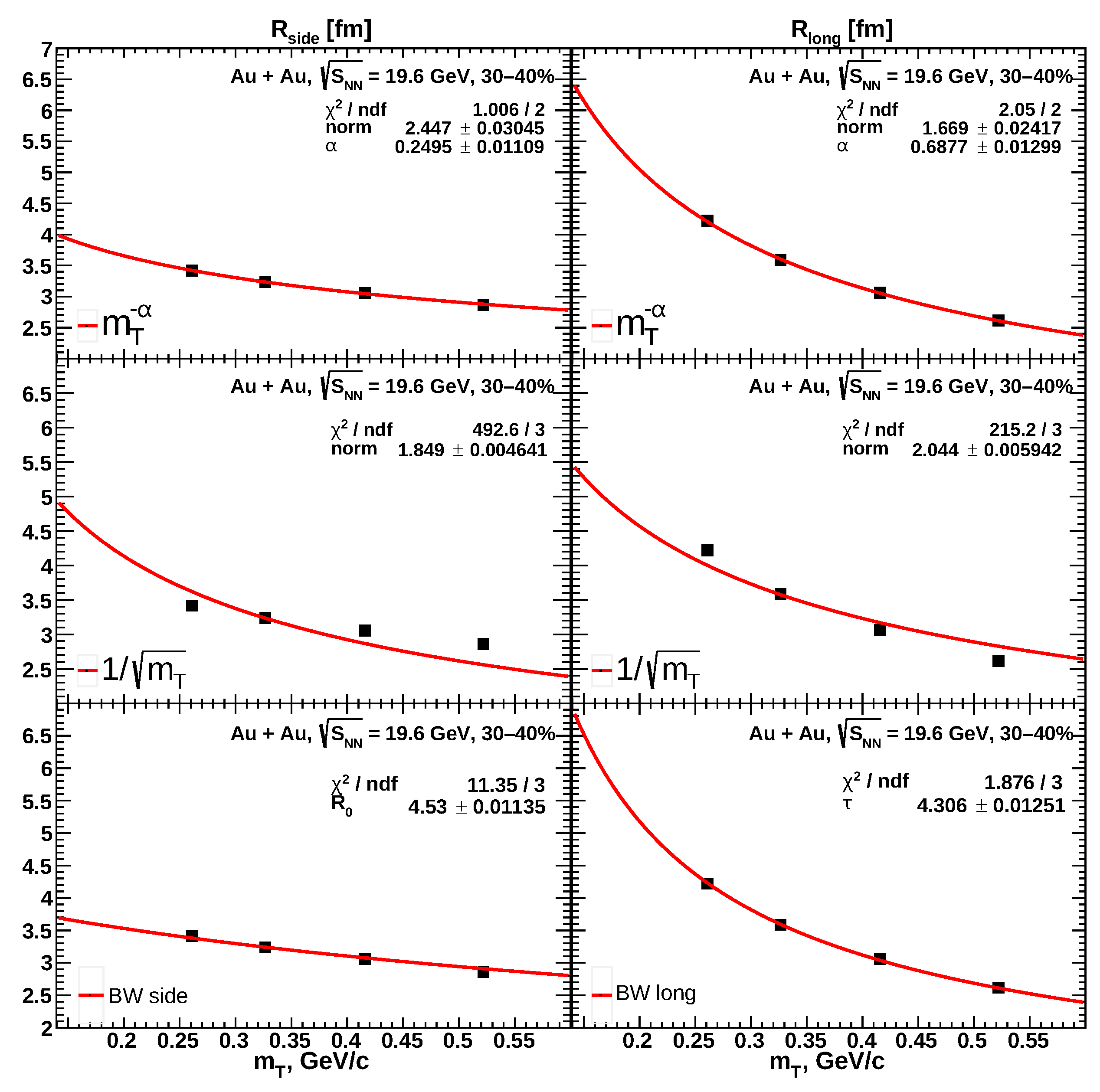
• The correlation function may deviate from a Gaussian shape due to exponential tails caused by resonance decay contributions [35]. This can lead to an underestimation of the femtoscopic radii.
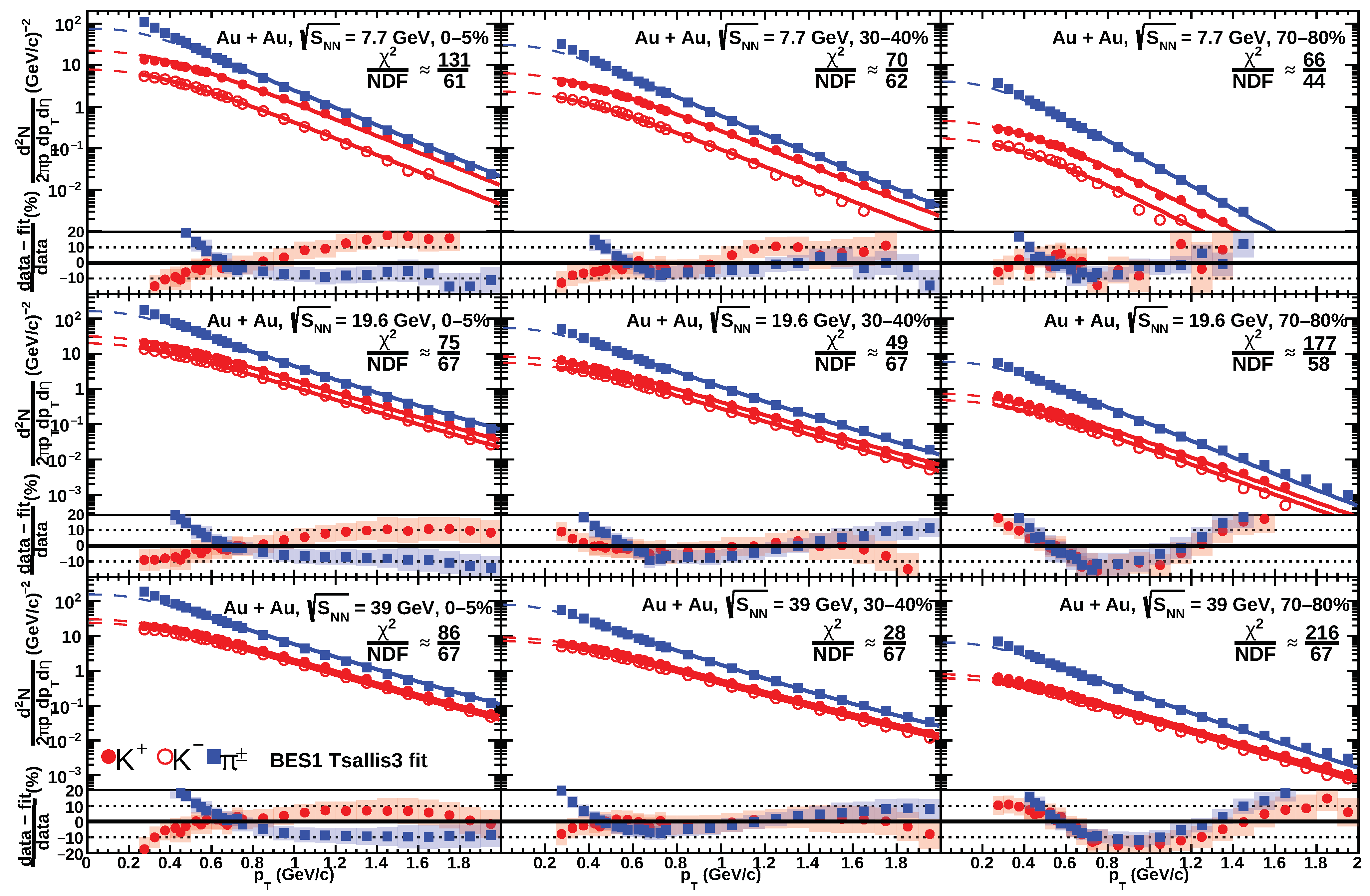
• In the Tsallis statistics, the particle interactions and collective effects, including rescattering, are modeled phenomenologically by deformation of entropy using the nonextensive entropic parameter q.

4. Conclusions

In this study, we compared two different methods for the determination of the size of the system formed in ultrarelativistic heavy-ion collisions at kinetic freeze-out using femtoscopy and a statistical approach based on the Tsallis distribution. A procedure for recalculating correlation radii was presented, ensuring proper comparison between the methods. The results show that collective effects, such as flow, strongly influence the femtoscopic radii. Simple models like $m_T$ scaling fail to describe these radii accurately, while the Blast-Wave model provides a better description.

One key finding is that femtoscopic volumes tend to be smaller than the volumes obtained in the Tsallis model, particularly at higher collision energies. This difference points to the need for further investigation, as it suggests potential underlying physics not fully captured by either method in their current forms.

Future work could refine this approach by calculating the system volume as the volume of a cylinder at kinetic freeze-out instead of relying on a simple product of radii. This might give more precise estimates and make the comparison between the two methods more reliable. Adding Tsallis statistics to the Blast-Wave framework could also help to improve the analysis.

Combining these methods can provide a more complete understanding of the system’s size and behavior. This will help to study possible phase transitions and better understand the properties of hot and dense matter in heavy-ion collisions.

References

1. BRAHMS Collaboration; Arsene, I.; Bearden, I.G.; Beavis, D.; Besliu, C.; Budick, B.; Bøggild, H.; Chasman, C.; Christensen, C.H.; Christiansen, P.; et al. Quark–gluon plasma and color glass condensate at RHIC? The perspective from the BRAHMS experiment. Nucl. Phys. A 2005, 757, 1–27. [Google Scholar] [CrossRef]
2. PHENIX Collaboration; Adcox, K.; Adler, S.S.; Afanasiev, S.; Aidala, C.; Ajitanand, N.N.; Akiba, Y.; Al-Jamel, A.; Alexander, J.; Amirikas, R.; et al. Formation of dense partonic matter in relativistic nucleus-nucleus collisions at RHIC: Experimental evaluation by the PHENIX collaboration. Nucl. Phys. A 2005, 757, 184–283. [Google Scholar] [CrossRef]
3. PHOBOS Collaboration; Back, B.B.; Baker, M.D.; Ballintijn, M.; Barton, D.S.; Becker, B.; Betts, R.R.; Bickley, A.A.; Bindel, R.; Budzanowski, A.; et al. The PHOBOS perspective on discoveries at RHIC. Nucl. Phys. A 2005, 757, 28–101. [Google Scholar] [CrossRef]
4. STAR Collaboration; Adams, J.; Aggarwal, M.M.; Ahammed, Z.; Amonett, J.; Anderson, B.D.; Arkhipkin, D.; Averichev, G.S.; Badyal, S.K.; Bai, Y.; et al. Experimental and theoretical challenges in the search for the quark-gluon plasma: The STAR collaboration’s critical assessment of the evidence from RHIC collisions. Nucl. Phys. A 2005, 757, 102–183. [Google Scholar] [CrossRef]
5. Aoki, Y.; Endrodi, G.; Fodor, Z.; Katz, S.D.; Szabo, K.K. The Order of the quantum chromodynamics transition predicted by the standard model of particle physics. Nature 2006, 443, 675–678. [Google Scholar] [CrossRef]
6. Bazavov, A.; Ding, H.T.; Hegde, P.; Kaczmarek, O.; Karsch, F.; Karthik, N.; Laermann, E.; Lahiri, A.; Larsen, R.; Li, S.-T.; et al. Chiral crossover in QCD at zero and non-zero chemical potentials. Phys. Lett. B 2019, 795, 15–21. [Google Scholar] [CrossRef]
7. Adamczyk, L.; Adkins, J.K.; Agakishiev, G.; Aggarwal, M.M.; Ahammed, Z.; Ajitanand, N.N.; Alekseev, I.; Anderson, D.M.; Aoyama, R.; Aparin, A.; et al. Bulk properties of the medium produced in relativistic heavy-ion collisions from the beam energy scan program. Phys. Rev. C 2017, 96, 044904. [Google Scholar] [CrossRef]
8. Adamczyk, L.; Adkins, J.K.; Agakishiev, G.; Aggarwal, M.M.; Ahammed, Z.; Alekseev, I.; Alford, J.; Anson, C.D.; Aparin, A. Beam-energy-dependent two-pion interferometry and the freeze-out eccentricity of pions measured in heavy ion collisions at the STAR detector. Phys. Rev. C 2015, 92, 014904. [Google Scholar] [CrossRef]
9. Tsallis, C. Possible generalization of Boltzmann-Gibbs statistics. J. Statist. Phys. 1988, 52, 479–487. [Google Scholar] [CrossRef]
10. Tsallis, C.; Mendes, R.S.; Plastino, A.R. The role of constraints within generalized nonextensive statistics. Phys. A 1998, 261, 534–554. [Google Scholar] [CrossRef]
11. Parvan, A.S. Hadron transverse momentum distributions in the Tsallis statistics with escort probabilities. J. Phys. G Nucl. Part. Phys. 2023, 50, 125002. [Google Scholar] [CrossRef]
12. Brown, R.H.; Twiss, R.Q. A Test of a New Type of Stellar Interferometer on Sirius. Nature 1956, 178, 1046–1048. [Google Scholar] [CrossRef]
13. Goldhaber, G.; Goldhaber, S.; Lee, W.; Pais, A. Influence of Bose-Einstein Statistics on the Antiproton-Proton Annihilation Process. Phys. Rev. 1960, 120, 300. [Google Scholar] [CrossRef]
14. Kopylov, G.I.; Podgoretsky, M.I. Correlations of identical particles emitted by highly excited nuclei. Sov. J. Nucl. Phys. 1972, 15, 219–223. [Google Scholar]
15. Lednicky, R.; Lyuboshits, V.L. Final State Interaction Effect on Pairing Correlations Between Particles with Small Relative Momenta. Sov. J. Nucl. Phys. 1982, 15, 770. [Google Scholar]
16. Kaufman, S.; Ashktorab, K.; Beavis, D.; Chasman, C.; Chen, Z.; Chu, Y.Y.; Cumming, J.B.; Debbe, R.; Gonin, M.; Gushue, S.; et al. System, centrality, and transverse mass dependence of two-pion correlation radii in heavy ion collisions at 11.6A and 14.6A GeV/c. Phys. Rev. C 2002, 66, 549061–5490615. [Google Scholar]
17. Bearden, I.G.; Bøggild, H.; Boissevain, J.; Dodd, J.; Erazmus, B.; Esumi, S.; Fabjan, C.W.; Ferenc, D.; Fields, D.E.; Franz, A.; et al. High energy Pb+Pb collisions viewed by pion interferometry. Phys. Rev. C 1998, 58, 1656. [Google Scholar] [CrossRef]
18. Adams, J.; Aggarwal, M.M.; Ahammed, Z.; Amonett, J.; Anderson, B.D.; Arkhipkin, D.; Averichev, G.S.; Badyal, S.K.; Bai, Y.; Balewski, J.; et al. Pion interferometry in Au+Au collisions at s NN =200 GeV. Phys. Rev. C 2005, 71, 044906. [Google Scholar] [CrossRef]
19. Aamodt, K.; Quintana, A.A.; Adamová, D.; Adare, A.M.; Aggarwal, M.M.; Rinella, G.A.; Rinella, G.A.; Agocs, A.G.; Salazar, S.A.; Ahammed, Z.; et al. Two-pion Bose–Einstein correlations in central Pb–Pb collisions at s NN =2.76 TeV. Phys. Lett. B 2011, 696, 328–337. [Google Scholar] [CrossRef]
20. Hatlo, M.; James, F.; Mato, P.; Moneta, L.; Winkler, M.; Zsenei, A. Developments of mathematical software libraries for the LHC experiments. IEEE Trans. Nucl. Sci. 2005, 52, 2818–2822. [Google Scholar] [CrossRef]
21. Lisa, M.; Pratt, S.; Soltz, R.; Wiedemann, U. Femtoscopy in Relativistic Heavy Ion Collisions: Two Decades of Progress. Ann. Rev. Nucl. Part. Sci. 2005, 55, 357–402. [Google Scholar] [CrossRef]
22. Pratt, S. Pion interferometry of quark-gluon plasma. Phys. Rev. D 1986, 33, 1314. [Google Scholar] [CrossRef]
23. Bertsch, G.; Gong, M.; Tohyama, M. Pion interferometry in ultrarelativistic heavy-ion collisions. Phys. Rev. C 1988, 37, 1896. [Google Scholar] [CrossRef] [PubMed]
24. Sinyukov, Y.M.; Lednicky, R.; Akkelin, S.V.; Pluta, J.; Erazmus, B. Coulomb corrections for interferometry analysis of expanding hadron systems. Phys. Lett. B 1998, 432, 248–257. [Google Scholar] [CrossRef]
25. Bowler, M.G. Coulomb corrections to Bose-Einstein corrections have greatly exaggerated. Phys. Lett. B 1991, 270, 69–74. [Google Scholar] [CrossRef]
26. Wiedemann, U.A.; Heinz, U. Particle interferometry for relativistic heavy-ion collisions. Phys. Rept. 1999, 319, 150–230. [Google Scholar] [CrossRef]
27. Makhlin, A.N.; Sinyukov, Y.M. Hydrodynamics of Hadron Matter Under Pion Interferometric Microscope. Z. Phys. C 1988, 39, 69. [Google Scholar] [CrossRef]
28. Wiedemann, U.A.; Scotto, P.; Heinz, U. Transverse momentum dependence of Hanbury-Brown–Twiss correlation radii. Phys. Rev. C 1996, 53, 918. [Google Scholar] [CrossRef]
29. Schnedermann, E.; Sollfrank, J.; Heinz, U. Thermal phenomenology of hadrons from 200A GeV S+S collisions. Phys. Rev. C 1993, 48, 2462. [Google Scholar] [CrossRef]
30. Retière, F.; Lisa, M.A. Observable implications of geometrical and dynamical aspects of freeze-out in heavy ion collisions. Phys. Rev. C 2004, 70, 044907. [Google Scholar] [CrossRef]
31. Heinz, U.W.; Tomasik, B.; Wiedemann, U.A.; Wu, Y.F. Lifetimes and sizes from two-particle correlation functions. Phys. Lett. B 1996, 382, 181. [Google Scholar] [CrossRef]
32. Nedorezov, E.V.; Parvan, A.S.; Aparin, A.A. Description of Charged Particle Dependence on Transverse Momentum with Tsallis-Like Distribution. Phys. Part. Nucl. 2024, 55, 984–989. [Google Scholar] [CrossRef]
33. Parvan, A.S. Equivalence of the phenomenological Tsallis distribution to the transverse momentum distribution of q-dual statistics. Eur. Phys. J. A 2020, 56, 106. [Google Scholar] [CrossRef]
34. Sinyukov, Y.M. Spectra and correlations in locally equilibrium hadron and quark-gluon systems. Nucl. Phys. A 1994, 566, 589–592. [Google Scholar] [CrossRef]
35. Shapoval, V.M.; Sinyukov, Y.M.; Karpenko, I.A. Emission source functions in heavy ion collisions. Phys. Rev. C 2013, 88, 064904. [Google Scholar] [CrossRef]
Figure 1. Tsallis-3 model fits of K ± , π ± at s NN = 7.7, 19.6, 39 GeV and the centrality classes 0–5%, 30–40%, 70–80%. Data points are taken from [7].
Particles 08 00034 g001
Figure 2. Femtoscopic π ± radii fits at s NN = 19.6 GeV and the centrality class 30–40% using Equations (8)–(10). Data points are taken from [8].
Particles 08 00034 g002
Figure 3. Comparison of volumes at s NN = 7.7, 19.6, 39 GeV and the centrality classes from 0–5% to 60–70% obtained using the Tsallis-3 statistics and calculated using Equations (8)–(10).
Particles 08 00034 g003
Disclaimer/Publisher’s Note: The statements, opinions and data contained in all publications are solely those of the individual author(s) and contributor(s) and not of MDPI and/or the editor(s). MDPI and/or the editor(s) disclaim responsibility for any injury to people or property resulting from any ideas, methods, instructions or products referred to in the content.