Vibration Minimisation of Moving Flexible Slender Structures Based on Time-Parameterised B-Spline

Abstract

Vibration mitigation of moving flexible structures is a key issue in many applications. Examples include antennas, solar arrays, radar reflectors, and manipulator arms, especially in the aerospace sector. These structures typically consist of inter-connected slender and flexible elements moved by external actuators to reach specific configurations and positions. The movements excite vibrations, which lead to the risk of structural and fatigue failures; once in position, residual vibrations can be further amplified by structure lightness, causing bad performance and malfunctioning of onboard sensors. This paper proposes an effective technique to minimise the vibration of moving flexible structures by calculating the control points of a time-parametrised B-spline representing the shape of the motion law. A testing case of a rotating cantilever beam is considered. Validation using multi-flexible-body simulation software has shown the method’s effectiveness in minimising residual vibrations.

1. Introduction

Vibration control of moving flexible slender structures is a key issue in many engineering applications. Some examples include, but are not limited to, the following: antennas, solar arrays, radar reflectors, and robotic arms, especially in the aerospace sector [1,2,3,4,5] or in manipulators mounted on moving platforms [6,7], where weight, compactness, and energy consumption are restrictive design constraints. These structures typically consist of interconnected slender and flexible elements that external actuators move to achieve specific configurations and positions. The motion law causes unwanted vibrations, with the risk of precision degradation and structural failure due to mechanical fatigue. Furthermore, vibrations can also affect the perception and sensing capabilities of robots. Sensory systems, such as cameras, lidars or other environmental sensors, can be susceptible to vibrations, leading to distorted or unreliable data acquisition. This has significant consequences for applications that rely on accurate sensing, such as autonomous navigation or object recognition. An example of this scenario is discussed in [7], where input-shaping techniques are applied to suppress the end-effector vibrations in a mobile mine-detecting robotic manipulator; in this case, due to the long reach of the arm mounted on the moving platform, unwanted oscillations can corrupt the scanning information collected by the sensor system positioned at the end of the arm.

The most common motion-control techniques for the reduction of vibrations induced in flexible structures by imposed motion can be broadly categorised into the two following groups:

-

open-loop control that involves generating motion trajectories [8] able to mitigate expected vibrations by foreseeing their effects before they occur. These techniques often utilise sophisticated control algorithms, such as input shaping and model-based control, to pre-calculate and optimise the desired motion profiles;

-

closed-loop control that employs sensors and actuators to measure and counteract vibrations in real time actively, e.g., [9]. These methods typically utilise feedback control algorithms to monitor the system’s response continuously and to generate appropriate control signals for damping the vibrations.

The method presented in this paper falls into the first group and in the pre-shaping techniques for motion control. Pre-shaping techniques can be highly effective in reducing vibrations, but they are prone to uncertainties and non-linear behaviours. On the other hand, closed-loop techniques can be affected by sensor noise and involve complex sensing and actuation systems, higher implementation costs, and increased system complexity and maintenance requirements. Therefore, these two techniques should be considered part of a more general hybrid approach to minimise vibrations. As an example, an interesting application of a hybrid methodology can be found in [10], where both joint trajectory planning, based on the LQR formalism, and collocated active control using piezoelectric actuation, for compensating modelling uncertainties, is applied to control a flexible link robot. It is worth saying that pre-shaping becomes the main applicable vibration control strategy when the system cannot be equipped with sensors or when sensors are not responding. An industrial example from the authors’ experience is a sorting system for laser-proceed sheets with dual-arm Cartesian kinematics [11]. In this application, the structure whose vibrations need to be minimised is a part of the system transported by the gripping tools and, for obvious technological reasons, its sensorisation is not a viable solution; therefore pre-shaped techniques of the motion profile must be implemented to improve the system performance and to reduce vibrations. In any case, pre-shaping the motion law can improve the accuracy and robustness of sensory inputs and enable the construction of lighter systems with reduced energy consumption at a design level. It follows that pre-shaping approaches should always be considered when the system’s dynamics can be predicted with relatively good accuracy, while at the same time, closed-loop control can be added to assure robustness, stability and performance, even in the presence of uncertainties and non-linearities. Many interesting studies on motion control using open- and closed-loop techniques for reducing self-induced vibration in flexible systems can be found in the literature, and a comprehensive literature review on the subject is beyond the scope of this paper. Therefore, only some studies are cited, while a general discussion and presentation of various techniques can be found, for example, in [12,13,14,15,16] or in books dedicated to the subject, e.g., [17].

One of the first studies on pre-shaped motion laws can be found in [18], where the vibration suppression problem was formulated as a mathematical optimisation in the mechanical cam profile design field. In [18], both linear and quadratic optimisations were evaluated, and the problem of constraining kinematics was addressed. Since then, a large number of algorithms and strategies have been developed and proposed in the literature, each with the potential to be efficacious in implementing vibration minimisation. The technique known as bang-bang control, in both its open- and closed-loop variations, has been a widely used strategy for vibration control of mechanical systems actuated by electric drives. Concerning its open-loop variant, the application requires accurate knowledge of the switching times, which can be obtained from a representative dynamic model of the system, e.g., [19]. Since the pre-shaped input law calculated using the bang-bang approach uses several discontinuities in the current profile supplied to the control, undesired oscillations and overshoot can occur, leading to sub-optimal power consumption. In [20], a bang-bang multi-switch time-optimal control technique was compared with an open-loop control function composed of a series of harmonics of ramped sinusoids, in terms of both residual vibration attenuation and actuation time; the methodologies were applied to a three-degree-of-freedom (DOF) mechanical model, concluding that the latter approach better satisfies both objectives. In [19], the bang-bang multi-switch method was studied on a continuous system consisting of a flexible robotic arm. Later, a different approach was proposed in [21], where a new method of pre-shaping the motion profile based on the gradient projection method was tested on two different flexible systems actuated by a servo DC motor. In this case, the acceleration law was described by a piece-wise constant function of time; despite the work’s contribution to the field, the same issues of bang-bang control related to profile discontinuities were not solved. A comparison between different pre-shaped motion profiles to reduce residual vibration in rest-to-rest movements of a flexible manipulator arm was discussed in [1], where the authors concluded that, compared to constant acceleration, a smoother motion profile consisting of sinusoidal arcs shows better performance in terms of vibration reduction. An interesting idea was proposed in [22], where an open-loop vibration control strategy that ensures high smoothness of the motion profile was applied to a mechanical servosystem with elastic transmission; however, despite considering constrained kinematics, the approach in [22] was limited to a single-DOF mechanical model and point-to-point tasks and could not be easily extended to more complex models and/or other design’s constraints such as interpolation of waypoints.

This work deals with the vibration minimisation induced in multi-mode flexible structures, such as translating or rotating flexible beams, actuated by a rigid joint. In the proposed approach, the motion imposed by the joint is obtained by appropriately calculating the control points of a time-parameterised B-spline representing the shape of the acceleration profile. The advantages of this parametrisation, which is universally accepted as a standard format in CAD applications, are well-known in the literature. Specifically, in a previous paper presented by the authors [23], time-parameterised B-splines are used as the data structure of a trajectory design framework based on the concept of iso-parametric representation of the motion profile. The parameterisation adopted is also particularly suitable in the case of defining motion with constrained kinematics by minimising a cost function using constrained minimisation techniques. Once the cost function has been defined, the motion constraints (typically the maximum velocities and accelerations imposed by the physical system) can easily be imposed as inequality constraints on the control polygon of the spline through linear combinations, e.g., [24,25,26].

The main contribution of this work is to provide a general methodology for extremely smooth pre-shaped control, increasing the knowledge in the literature on this type of method and attempting to meet the requirements of real industrial control. It is in fact demonstrated, also in the cited literature, that a smoother motion profile facilitates set-point tracking by the controller, resulting in higher performance. Compared to similar methods, the proposed technique allows the motion to be planned within the kinematic constraints imposed by the physical system and it can be easily extended to other types of constraints, such as interpolation of waypoints. The extreme flexibility of the approach also allows for other possible extensions, such as the use of multi-objective cost functions, or the control of more complex structures (implementing for example finite element models). While most of the similar techniques reported in the literature are limited to rest-to-rest applications, the method presented in this work is also suitable for defining multi-target motion profiles, especially when used in combination with an iso-parametric trajectory planning approach [23].

The remainder of the paper is organised as follows. Section 2 reports the mathematical theory of the proposed approach. Section 3 illustrates the specific application case to which the presented method is applied. In order to prove the validity of the method, a multibody simulation is presented and discussed in Section 4. Finally, a summary concludes this work in Section 5.

2. Method: Vibration Optimal Trajectory Planning

The methodology presented in this section is proposed for a one-axis application that can be modelled by one actuated rigid joint (prismatic or revolute) and flexible or rigid structures, which can be connected to each other by other joints. Typical examples of these models are translating or rotating flexible beams or lumped multi-degrees of freedom systems with rotational or translational motion such as pendulums and chains of mass springs. In all these cases, the dynamics can be generally modelled according to the following discretised equation

$$\mathit{M}\ddot{\mathit{y}}+\mathit{K}\mathit{y}=\mathbf{\Gamma }a\left(t\right),$$

(1)

where $\mathit{M}$ and $\mathit{K}$ are square mass and stiffness matrices, $a\left(t\right)$ is the acceleration imposed on the system by the actuator, $\mathbf{\Gamma }$ is a vector depending on the moving system and $\mathit{y}$ is a vector of generalised coordinates. The latter can be physical displacements, nodal displacements of an FE model of the structure or other coordinates such as modal coordinates of an assumed-mode model.

The system considered is linear, and the mass and stiffness matrices are real, symmetric and positive-definite. Therefore, a generalised eigenvalue decomposition can be applied to diagonalise the $\mathit{M}$ and $\mathit{K}$ matrices. Once the eigenvalues, ${\omega }_r$, and the normalised eigenvectors matrix, $\mathbf{\Phi }$, are evaluated, one can rewrite the system of uncoupled equations of motion in the eigenspace as

$${\ddot{q}}_r+{\omega }_r^2{q}_r={\gamma }_{r}a\left(t\right),\mathrm{with}:r=1,\dots ,n,\mathrm{and}{\gamma }_r=\sum _{j=1}^n{\mathbf{\Phi }}_{r,j}{\mathrm{\Gamma }}_r,$$

(2)

where n is the number of degrees of freedom (DOFs) in Equation (1).

If the acceleration profile $a\left(t\right)$ is known, Equation (2) can be solved by means of a convolution integral (Duhamel’s integral) [27]. Setting the initial conditions $q_r\left(0\right)=0$ and ${\dot{q}}_r\left(0\right)=0$, the response in the modal coordinates is as follows:

$$q_r\left(t\right)={\int }_0^t\frac{sin\left({\omega }_r(t-\tau )\right)}{{\omega }_r}{\gamma }_{r}a\left(\tau \right)d\tau .$$

(3)

Let $a\left(t\right)$ be defined by a 1D time-parameterised spline of degree d in its B-form

$$a\left(t\right)=\sum _{i=0}^m{B}_{i,d,\mathit{t}}\left(t\right)b_i,t\in [0,t_f],$$

(4)

where $t_f$ is the final time instant of the motion and $\mathit{b}=[b_0,\dots ,b_m]$ is the vector of control points. The basis functions $B_{i,d,\mathit{t}}\left(t\right)$ are defined by Cox-de Boor recursion formula [28]:

$$\left\{\begin{array}{c}{B}_{i,0,\mathit{t}}\left(t\right)=\left\{\begin{array}{cc}1,\hfill & \mathrm{if}{t}_i\le t<t_{i+1}\hfill \\ 0,\phantom{-}\hfill & \mathrm{otherwise}\hfill \end{array}\right.\hfill \\ B_{i,d,\mathit{t}}\left(t\right)={\displaystyle \frac{t-t_i}{t_{i+d}-t_i}}{B}_{i,d-1,\mathit{t}}\left(t\right)+{\displaystyle \frac{t_{i+d+1}-t}{t_{i+d+1}-t_{i+1}}}{B}_{i+1,d-1,\mathit{t}}\left(t\right)\hfill \end{array}\right.$$

(5)

based on a non-decreasing knot sequence $\mathit{t}=[t_0,\dots ,t_{m+d+1}]$. In this work, the knots are always non-periodic and non-uniform, i.e., in the form:

$$\mathit{t}=\{\underset{d+1}{\underbracket{0,\dots ,0}},t_{d+1},\dots ,t_m,\underset{d+1}{\underbracket{t_f,\dots ,t_f}}\}$$

(6)

with the endpoints of the parameterisation interval repeated $d+1$ times. Using Equation (4), the modal response in Equation (3) becomes

$$\begin{array}{c}\hfill \begin{array}{cc}\hfill q_r\left(t_f\right)& =\frac{1}{{\omega }_r}{\int }_0^{t_f}sin\left({\omega }_r(t_f-\tau )\right){\gamma }_{r}a\left(\tau \right)d\tau \hfill \\ \hfill & =\frac{{\gamma }_r}{{\omega }_r}{\int }_0^{t_f}sin\left({\omega }_r(t_f-\tau )\right)\left[\sum _{i=0}^m{B}_{i,d,\mathit{t}}\left(\tau \right)b_i\right]d\tau \hfill \\ \hfill & ={\int }_0^{t_f}f\left(\tau \right)\left[\sum _{i=0}^m{B}_{i,d,\mathit{t}}\left(\tau \right)b_i\right]d\tau .\hfill \end{array}\end{array}$$

(7)

Denoting by $D^{\left(i\right)}g\left(x\right)$ the i^th derivative of the generic function $g\left(x\right)$ and by $D^{(-i)}g\left(x\right)$ its i^th antiderivative, we proceed integrating by parts:

$$\begin{array}{c}\hfill \begin{array}{cc}\hfill {\int }_0^{t_f}f\left(\tau \right)a\left(\tau \right)d\tau =& D^{(-1)}f\left(t_f\right)a\left(t_f\right)-D^{(-1)}f\left(0\right)a\left(0\right)-\hfill \\ \hfill & {\int }_0^{t_f}{D}^{(-1)}f\left(\tau \right)D^{\left(1\right)}a\left(\tau \right)d\tau .\hfill \end{array}\end{array}$$

(8)

Since the d^th antiderivative of $f\left(\tau \right)$ is always defined, Equation (8) can be applied repeatedly to the integrand of Equation (7). As a consequence, the degree of the spline, resulting from the i^th derivation of $a\left(t\right)$, decreases consecutively until the degree is zero [29]. Imposing the boundary conditions

$${\left.D^{\left(i\right)}a\left(\tau \right)\right|}_{\tau =0}={\left.D^{\left(i\right)}a\left(\tau \right)\right|}_{\tau =t_f}=0i=0,\dots ,d-1,$$

(9)

the constant terms in Equation (8) become null, and Equation (7) can be written as follows:

$$q_r\left(t_f\right)={(-1)}^d\frac{{\gamma }_r}{{\omega }_r}{\int }_0^{t_f}{D}^{(-d)}\left(sin\left({\omega }_r(T-\tau )\right)\right)\left[\sum _{i=0}^{m-d}{B}_{i,0,{\mathit{t}}^{\left(d\right)}}\left(\tau \right)b_i^{\left(d\right)}\right]d\tau ,$$

(10)

where the knots ${\mathit{t}}^{\left(d\right)}=\{0,t_{d+1},\dots ,t_m,t_f\}$ are defined by setting the initial and final knots with a multiplicity of one in Equation (6) and obtained from the general formulation

$${\mathit{t}}^{\left(r\right)}=\{\underset{d-r+1}{\underbracket{0,\dots ,0}},t_{d+1},\dots ,t_m,\underset{d-r+1}{\underbracket{t_f,\dots ,t_f}}\}.$$

(11)

In Equation (10), the terms $b_i^{\left(d\right)}$ denote the control points of the d^th derivative of the spline $a\left(t\right)$, defined by the recursion formula [28]:

$$b_i^{\left(r\right)}=\sum _{j=i}^{i+r}{c}_{i,j}{b}_j=\left\{\begin{array}{cc}{b}_i\hfill & r=0\hfill \\ \frac{d-r+1}{t_{i+d+1}-t_{i+r}}\left(b_{i+1}^{(r-1)}-b_i^{(r-1)}\right)\hfill & r>0\hfill \end{array}\right.,$$

(12)

where $c_{i,j}$ is a constant. From Equation (5), we note that the terms $B_{i,0,{\mathit{t}}^{\left(d\right)}}\left(\tau \right)$ in Equation (10) is equal to 1 if the variable $\tau \in [t_i,t_{i+1}]$; otherwise, it is zero. It follows that, by the additive property of the integration operator, one obtains

$$\begin{array}{c}\hfill \begin{array}{cc}\hfill q_r\left(t_f\right)& ={(-1)}^d\sum _{i=0}^{m-d}\frac{{\gamma }_r{b}_i^{\left(d\right)}}{{\omega }_r}{\int }_{t_{i+d}}^{t_{i+d+1}}{D}^{(-d)}\left[sin\left({\omega }_r(t_f-\tau )\right)\right]d\tau \hfill \\ \hfill & ={(-1)}^d\sum _{i=0}^{m-d}\frac{{\gamma }_r{b}_i^{\left(d\right)}}{{\omega }_r}{\left[D^{(-d-1)}\left[sin\left({\omega }_r(t_f-\tau )\right)\right]\right]}_{t_{i+d}}^{t_{i+d+1}}.\hfill \end{array}\end{array}$$

(13)

Defining:

$$a_{r,i}=\frac{{\gamma }_r}{{\omega }_r}{\left[D^{(-d-1)}\left[sin\left({\omega }_r(t_f-\tau )\right)\right]\right]}_{t_{i+d}}^{t_{i+d+1}},$$

(14)

we can expand Equation (13) to obtain a linear combination of the elements of the unknown vector $\mathit{b}$:

$$\begin{array}{c}\hfill \begin{array}{cc}\hfill q_r\left(t_f\right)& ={(-1)}^d\sum _{i=0}^{m-d}\left(a_{r,i}\sum _{j=i}^{i+d}{c}_{i,j}{b}_j\right)\hfill \\ \hfill & ={(-1)}^d\sum _{j=0}^m{b}_j\left(\sum _{i=max(0,j-d)}^{min(m-d,j)}{a}_{r,i}{c}_{i,j}\right)={(-1)}^d\sum _{j=0}^m{b}_j{\overline{q}}_{r,j}.\hfill \end{array}\end{array}$$

(15)

Repeating the same passages and similarly to how Equation (15) is derived, the time derivatives of Equation (3) at $t_f$ is reformulated as

$$\begin{array}{c}\hfill \begin{array}{cc}\hfill {\dot{q}}_r\left(t\right)=& \frac{d}{dt}\left(\frac{1}{{\omega }_r}{\int }_0^{t}sin\left({\omega }_r(t-\tau )\right){\gamma }_{r}a\left(\tau \right)d\tau \right)\hfill \\ \hfill & ={\gamma }_r{\int }_0^{t}cos\left({\omega }_r(t-\tau )\right)a\left(\tau \right)d\tau \hfill \\ \hfill & ={\dot{q}}_r\left(t_f\right)={(-1)}^d\sum _{j=0}^m{b}_j{\dot{\overline{q}}}_{r,j},\hfill \end{array}\end{array}$$

(16)

where

$$\begin{array}{cc}\hfill & {\dot{\overline{q}}}_{r,j}=\sum _{i=max(0,j-d)}^{min(m-d,j)}{\dot{a}}_{r,i}{c}_{i,j}\hfill \end{array}$$

(17)

$$\begin{array}{cc}\hfill & {\dot{a}}_{r,i}={\gamma }_r{\left[D^{(-d-1)}\left[cos\left({\omega }_r(T-\tau )\right)\right]\right]}_{t_{i+d}}^{t_{i+d+1}}.\hfill \end{array}$$

(18)

The residual energy of the system at time $t_f$ can be expressed by

$$E_{res}\left(\mathit{b}\right)=\frac{1}{2}\sum _{r=1}^n\left[{\dot{q}}_r^2\left(t_f\right)+{\omega }_r^2{q}_r^2\left(t_f\right)\right]=\frac{1}{2}{\mathit{b}}^T\left(\sum _{r=1}^n{\mathit{H}}_r\right)\mathit{b},$$

(19)

where ${\mathit{H}}_r$ is the symmetric matrix:

$${\mathit{H}}_r=\left[\begin{array}{cccc}{\omega }_r^2{\overline{q}}_{r,0}^2+{\dot{\overline{q}}}_{r,0}^2& {\omega }_r^2{\overline{q}}_{r,0}{\overline{q}}_{r,1}+{\dot{\overline{q}}}_{r,0}{\dot{\overline{q}}}_{r,1}& \dots & {\omega }_r^2{\overline{q}}_{r,0}{\overline{q}}_{r,m}+{\dot{\overline{q}}}_{r,0}{\dot{\overline{q}}}_{r,m}\\ {\omega }_r^2{\overline{q}}_{r,1}{\overline{q}}_{r,0}+{\dot{\overline{q}}}_{r,1}{\dot{\overline{q}}}_{r,0}& {\omega }_r^2{\overline{q}}_{r,1}^2+{\dot{\overline{q}}}_{r,1}^2& \dots & {\omega }_r^2{\overline{q}}_{r,1}{\overline{q}}_{r,m}+{\dot{\overline{q}}}_{r,1}{\dot{\overline{q}}}_{r,m}\\ ⋮& ⋮& \ddots & ⋮\\ {\omega }_r^2{\overline{q}}_{r,m}{\overline{q}}_{r,0}+{\dot{\overline{q}}}_{r,m}{\dot{\overline{q}}}_{r,0}& {\omega }_r^2{\overline{q}}_{r,m}{\overline{q}}_{r,1}+{\dot{\overline{q}}}_{r,m}{\dot{\overline{q}}}_{r,1}& \dots & {\omega }_r^2{\overline{q}}_{r,m}^2+{\dot{\overline{q}}}_{r,m}^2.\end{array}\right].$$

(20)

Since Equation (19) is in standard quadratic form, it follows that

$$\mathit{H}=\sum _{r=1}^n{\mathit{H}}_r={\nabla }^2{E}_{res}\left(\mathit{b}\right).$$

(21)

From the definition of residual energy, we have $E_{res}\left(\mathit{b}\right)\ge 0\forall \mathit{b}$; therefore, the matrix $\mathit{H}$ is positive semi-definite and the residual energy in Equation (19) is convex. Consequently, the determination of the unknown control points $\mathit{b}$ can be obtained using convex quadratic minimisation. The Hessian matrix $\mathit{H}$ is uniquely defined by the adopted knots $\mathit{t}$ and the coefficients $c_{i,j}$, $a_{r,i}$, and ${\dot{a}}_{r,i}$. Appendix A shows these coefficients up to degree 2 of the spline. The knots sequence $\mathit{t}$ adopted in this work is obtained by averaging the formula from an equispaced mesh in the parametric domain, in accordance with the following expressions:

$$\begin{array}{c}\hfill \begin{array}{cc}\hfill & t_0=\cdots =t_d=0,t_{m+1}=\cdots =t_{m+d+1}=t_f,\hfill \\ \hfill & t_{j+d}=\frac{1}{max(d,1)}\sum _{i=j}^{j+d-1}\left[\frac{i}{m}{t}_f\right],j=1\dots ,m-d.\hfill \end{array}\end{array}$$

(22)

In practical applications, the motion profile is subject to physical constraints dictated by the mechanics of the system and the specific drive, in addition to the requirements of the desired trajectory. For the sake of clarity, we define the position, velocity and jerk profiles: $p\left(t\right)=D^{(-2)}a\left(t\right)$, $v\left(t\right)=D^{(-1)}a\left(t\right)$, and $j\left(t\right)=D^{\left(1\right)}a\left(t\right)$. Constant kinematic limits $VC$, $AC$ and $JC$ are assumed for the velocity, acceleration and jerk constraints, respectively. Let $\Delta p=p_t-p_s$ and $\Delta v=v_t-v_s$ be defined, with the subscripts s and t corresponding to the start and target states of the system. Since the problem is not limited to these constraints, in this work we considered the following:

$$\left\{\begin{array}{c}p\left(0\right)=p_s,p\left(t_f\right)=p_t,\hfill \\ v\left(0\right)=v_s,v\left(t_f\right)=v_t,\hfill \\ a\left(0\right)=0,a\left(t_f\right)=0,\hfill \\ j\left(0\right)=0,j\left(t_f\right)=0,\hfill \\ {0\le v\left(t\right)|}_{[0,t_f]}\le VC,\hfill \\ \underset{t\in [0,t_f]}{max}\left|a\left(t\right)\right|\le AC,\hfill \\ \underset{t\in [0,t_f]}{max}\left|j\left(t\right)\right|\le JC.\hfill \end{array}\right.$$

(23)

Other constraints can be included in (23); for example, it may be desired to pass through some positions (or any derivative) that can be expressed as interpolation constraints.

A spline of degree d is always contained in the convex hull of its control polygon. It follows that it is conservative to express Equation (23) as linear relations of the control points $\mathit{b}$ of the spline $a\left(t\right)$ [24,25,26]. The constrained QP problem can be summarised as follows:

$$\begin{array}{c}\hfill \begin{array}{cc}\hfill & \mathit{minimise}:E_{res}\left(\mathit{b}\right),\hfill \\ \hfill & \mathit{subject}\mathit{to}:\mathit{l}\le \mathit{C}\mathit{b}\le \mathit{u},\hfill \end{array}\end{array}$$

(24)

where $\mathit{C}$ is the constraints matrix, while the vectors $\mathit{l}$ and $\mathit{u}$ are the lower and upper limits and they are defined as follows:

$$\mathit{C}=\left[\begin{array}{c}{\mathit{D}}^{+}\\ \mathit{I}\\ {\mathit{D}}^{-}\\ \mathit{S}\end{array}\right]\in {\mathbb{R}}^{3(m+1)\times m+1},$$

(25)

with $\mathit{I}$ identity matrix and

$$\begin{array}{cc}\hfill & {\mathit{D}}^{+}=\left[\begin{array}{ccccc}-\frac{d}{t_{d+1}-t_1}& \frac{d}{t_{d+1}-t_1}& & \dots & 0\\ & -\frac{d}{t_{d+2}-t_2}& \frac{d}{t_{d+2}-t_2}& & ⋮\\ ⋮& & \ddots & \ddots & \\ 0& \dots & & -\frac{d}{t_{m+d}-t_m}& \frac{d}{t_{m+d}-t_m}\end{array}\right],\hfill \end{array}$$

(26)

$$\begin{array}{cc}\hfill & {\mathit{D}}^{-}=\left[\begin{array}{ccccccc}\frac{t_{d+1}-t_0}{d+1}& & & & \dots & & 0\\ \frac{t_{d+1}-t_0}{d+1}& \frac{t_{d+2}-t_1}{d+1}& & & & & ⋮\\ ⋮& & \ddots & & & & \\ & & & \frac{t_{d+1+j}-t_j}{d+1}& & & \\ ⋮& & & & \ddots & & \\ \frac{t_{d+1}-t_0}{d+1}& \dots & & \frac{t_{d+1+j}-t_j}{d+1}& \dots & & \frac{t_{d+m+1}-t_m}{d+1}\end{array}\right],\hfill \end{array}$$

(27)

$$\begin{array}{cc}\hfill & \mathit{S}={\left(\sum _{j=0}^{m-i}\frac{t_{d+1+i}-t_i}{d+1}\frac{t_{d+2+j}^{(-1)}-t_j^{(-1)}}{d+2}\right)}_{i=0}^m,\hfill \end{array}$$

(28)

$$\begin{array}{cc}\hfill & \mathit{l}=[0,\underset{m-2}{\underbracket{-JC,\dots ,-JC}},0,0,\underset{m-1}{\underbracket{-AC,\dots ,-AC}},0,\underset{m}{\underbracket{-v_s,\dots ,-v_s}},\Delta v,\Delta p-v_s{t}_f],\hfill \end{array}$$

(29)

$$\begin{array}{cc}\hfill & \mathit{u}=[0,\underset{m-2}{\underbracket{JC,\dots ,JC}},0,0,\underset{m-1}{\underbracket{AC,\dots ,AC}},0,\underset{m}{\underbracket{VC-v_s,\dots ,VC-v_s}},\Delta v,\Delta p-v_s{t}_f].\hfill \end{array}$$

(30)

The ${\mathit{D}}^{+}$ matrix is derived from Equation (12), while more details about ${\mathit{D}}^{-}$ and $\mathit{S}$ are provided in Appendix B.

The problem defined by Equation (24) can be solved using a standard quadratic minimisation solver. In this work, the solution is computed with an Operator splitting Solver for convex Quadratic Programs (OSQP) [30]. The OSQP solver needs the $\mathit{H}$ and $\mathit{C}$ matrices provided in the Compressed Sparse Column (CSC) format. A comprehensive explanation of the storage CSC format can be found in reference [31]. In particular, for the $\mathit{H}$ matrix, only its upper triangular part is required.

We conclude this section with a consideration on the limits of applicability of the proposed method. Specifically, a solution that satisfies the constraints is not always possible when the time $t_f$ is insufficient to perform the displacement $\Delta p$ satisfying both the kinematic constraints and the required smoothness of the motion profile. In this case, a solution is to increase either $t_f$, the number of control points or both until an acceptable value of the cost function in (19) is obtained. A more refined solution would instead consist of appropriately modifying (19) to define a multi-objective cost function that also introduces $\mathit{t}$ knots into the problem variables. This solution, although of interest to the authors, will not be explored in this paper but will be the subject of future work.

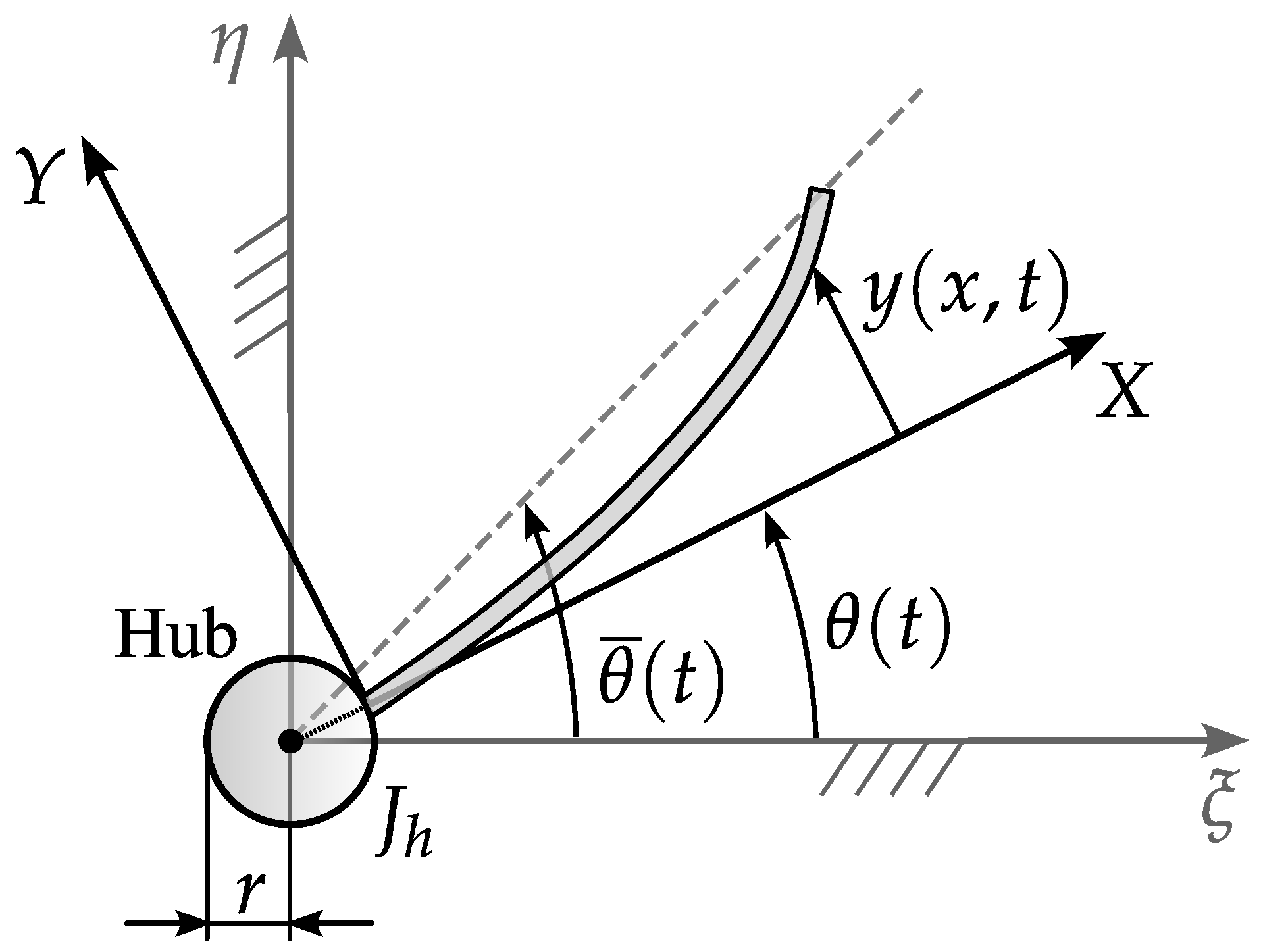
3. Testing Case: A Rotating Multi-Mode Flexible and Slender Beam

Mechanical systems that consist of thin or slender flexible structures can be effectively represented by beam or rod models. Therefore, to test the method’s effectiveness, we designed the acceleration input laws to control the endpoint position of a flexible beam of length L attached to a rigid revolute joint of moment of inertia $J_h$ and radius r (Figure 1).

The motion of the beam is constrained to the horizontal plane, and gravity is not considered. To describe the flexural vibration of the beam, two Cartesian systems of coordinates are used: the fixed inertia coordinates $(\xi ,\eta )$ and the relative coordinates $(X,Y)$ rotating around the joint axis, as shown in Figure 1. During the movement, the beam undergoes rigid body motion defined by $\theta \left(t\right)$, while $\overline{\theta }\left(t\right)$ represents the angular displacement of the beam’s endpoint.

Both the shear and rotatory inertia effects are neglected. The link is represented by an Euler–Bernoulli beam whose mass per unit length and Young’s modulus are denoted by $\rho$ and E, respectively; $y(x,t)$ is the transverse displacement of the beam measured in the relative frame $(X,Y)$. The control aims to minimise the beam’s tip-point residual vibrations that result from the motion law $\ddot{\theta }\left(t\right)$ due to the application and release of the motion generated by the actuator in the hub.

The complex dynamics of this system have been extensively studied in the literature, e.g., [32,33,34,35,36,37,38], and details on the full development of the equations of motion are not reported here. We assume that the angular velocity $\dot{\theta }\left(t\right)$ and the beam deflection $y(x,t)$ are relatively small so that centrifugal and Coriolis effects can be neglected [33]. Under these premises, the governing equation of motion of the beam could be simplified as follows:

$$EI\frac{{\partial }^{4}y}{\partial x^4}+\rho \frac{{\partial }^{2}y}{\partial t^2}=-\rho x\ddot{\theta }.$$

(31)

To obtain an approximate formulation of the Equation (31), we assume the solution in the form of a series composed by a linear combination of admissible functions ${\mathrm{\Phi }}_i$, multiplied by time-dependent generalised coordinates $q_i$ [27]:

$$y(x,t)=\sum _{i=1}^n{\mathrm{\Phi }}_i\left(x\right)q_i\left(t\right).$$

(32)

The eigenfunctions of a clamped-free beam are used as admissible functions:

$${\mathrm{\Phi }}_i\left(x\right)=K_i[sin\left({\beta }_{i}x\right)-sinh\left({\beta }_{i}x\right)-{\alpha }_i(cos\left({\beta }_{i}x\right)-cosh\left({\beta }_{i}x\right))],$$

(33)

where

$${\alpha }_i=\frac{sin\left({\beta }_{i}L\right)+sinh\left({\beta }_{i}L\right)}{cos\left({\beta }_{i}L\right)+cosh\left({\beta }_{i}L\right)}$$

(34)

and $\beta$ is obtained from the characteristic equation

$$cos\left({\beta }_{i}L\right)cosh\left({\beta }_{i}L\right)+1=0.$$

(35)

Six modes are assumed in the problem, resulting in a $6\times 6$ problem in Equation (1). More or less modes can be chosen according to the problem and the analyst’s choice. Substituting Equation (32) into Equation (31) and premultiplying by ${\mathrm{\Phi }}_j\left(x\right)$, after integration over the domain $[r,r+L]$, the discretised equations of motion in the form of Equation (1) are obtained, where the mass $\mathit{M}$ and stiffness $\mathit{K}$ matrices and the vector $\mathbf{\Gamma }$ in Equation (1) are

$$\begin{array}{c}\hfill {\mathit{M}}_{i,j}={\int }_r^{r+L}\rho {\mathrm{\Phi }}_i{\mathrm{\Phi }}_{j}dx,{\mathit{K}}_{i,j}={\int }_r^{r+L}EI{\mathrm{\Phi }}_i^{″}{\mathrm{\Phi }}_j^{″}dx,{\mathbf{\Gamma }}_i=-{\int }_r^{r+L}\rho x{\mathrm{\Phi }}_{i}dx.\end{array}$$

(36)

Material and geometrical data of the beam are given in

Table 1. Material and geometrical data of the beam.

Cross section	$0.1$ m $\times 0.004$m
Length	$1$m
Young’s Modulus	$7\times {10}^{10}$N/m2
Material density	$2.62\times {10}^3$kg/m3
Hub radius	$0.1$m
Hub rotary inertia	$1$kg/m2

.

Two different scenarios are considered: the first deals with rest-to-rest motion profiles; the second proposes an application of our algorithm to a multi-target problem.

3.1. Rest-to-Rest Testing Case

In this scenario, the algorithm detailed in Section 2 is tested on rest-to-rest motion profiles, thus using the conditions $p_s=0,p_t=\Delta \theta$ and $v_s=v_t=$ 0. The proposed method is tested by varying some parameters; in particular, two cases are considered:

-

Case I: angular displacement $\Delta \theta =\pi /3$, change in actuation time $t_f$;

-

Case II: actuation time $t_f=1\mathrm{s}$, change in angular displacement $\Delta \theta$.

In more detail, the displacements and actuation times used in the tests are reported in

Table 2. Input data and performance data of the rest-to-rest testing case.

	Input Data			Performance Data
	$\Delta \mathit{\theta }$	${\mathit{t}}_{\mathit{f}}$	$\mathit{m}$ a	Solve Time b	Cost Func. (19)	Num. of Iterations
	[rad]	[s]	[-]	[ms]	[-]	[-]
	$\pi /3$	0.5	66	371.70	$9.4\times {10}^{-10}$	24,050
Case I	$\pi /3$	1.0	66	3.19	$9.5\times {10}^{-10}$	100
	$\pi /3$	1.5	66	2.69	$1.4\times {10}^{-10}$	75
	$\pi /6$	1.0	66	2.79	$6.8\times {10}^{-11}$	100
Case II	$\pi /3$	1.0	66	3.19	$9.5\times {10}^{-10}$	100
	$\pi /2$	1.0	66	4.61	$2.0\times {10}^{-10}$	275

a. Number of control points in acceleration derivation order. b. The operations have been computed on an Intel^® Core™ i7-10510U CPU, 1.80 GHz and 16 GB of RAM.

. The following kinematic constraints were used in all cases: $VC=3.5$ rad/s, $AC=30$ rad/s² and $JC=500$ rad/s³.

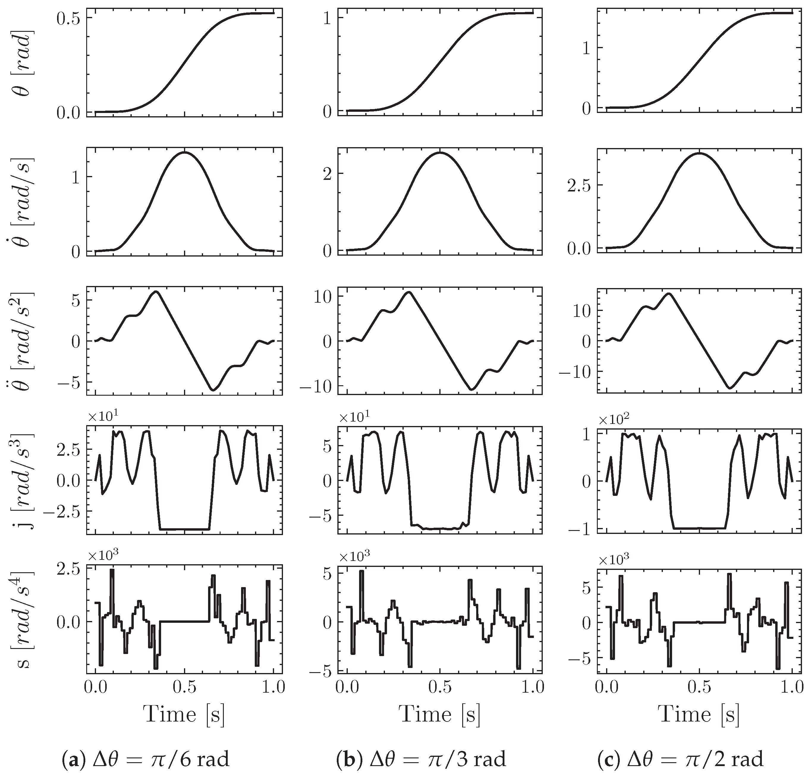
Figure 2 and Figure 3 show the optimal motion profiles obtained with the present method for Case I and Case II. The figures report the shapes of the position, velocity, acceleration, jerk and snap profiles (snap is the fourth time-derivative of the position). Table 2 also presents performance data related to the proposed motion law optimisation process. It can be noted that the solve time of the OSQP solver increases when the kinematic constraints become more severe and the actuation time is reduced. This condition, in fact, corresponds to more iterations of the solver and to an increase in the computational time.

3.2. Multi-Target Testing Case

In order to show the applicability of the methodology to multi-target applications, an optimised motion law for the minimisation of the vibrations at three distinct instants during the movements is presented. In this example, the desired motion profile consists of five sections: three with variable velocity, one with a constant velocity and one at zero velocity and acceleration (rest section). Such conditions occur in various application cases, such as those where a constant speed, or a rest condition, is required for the production process, e.g., a homogeneous layer for paint robots, static measurements, etc. In these cases, oscillations are undesired since they can compromise performance and quality.

The data for the different tasks are detailed in

Table 3. Input data and performance data of the multi-target testing case.

Task	Input Data						Performance Data
	${\mathit{p}}_{\mathit{s}}$	${\mathit{p}}_{\mathit{t}}$	${\mathit{v}}_{\mathit{s}}$	${\mathit{v}}_{\mathit{t}}$	$\Delta {\mathit{\tau }}_{\mathit{i}}$	m a	Solve	Cost Func.	Num. of
							Time b	(19)	Iterations
	[rad]	[rad]	[rad/s]	[rad/s]	[s]	[-]	[s]	[-]	[-]
1	0	$\pi /3$	0	2	$0.7$	51	$24.1$	$6.1\times {10}^{-13}$	$3,600,775$
2	$\pi /3$	$5\pi /6$	2	2	$0.785$	3	-	-	-
3	$5\pi /6$	$\pi$	2	0	$0.5$	51	$40.7$	$3.5\times {10}^{-12}$	$6,033,250$
4	$\pi$	$\pi$	0	0	1	3	-	-	-
5	$\pi$	0	0	0	$1.65$	76	$21.6$	$2.4\times {10}^{-13}$	$1,595,900$

a. Number of control points in acceleration derivation order. b. The operations have been computed on an Intel^® Core™ i7-10750H CPU, 2.60 GHz and 16 GB of RAM.

. The following kinematic constraints were adopted for the entire motion profile: $VC=3.5$ rad/s, $AC=10$ rad/s² and $JC=70$ rad/s³. All sections are defined by time-parametrised B-splines of degree $d=4$, relative to the position order, and post-processed through the framework proposed in [23] in order to obtain a motion profile described by a single parametric function.

The shape of the generated motion profile, from position to jerk, is shown in Figure 4, where $\Delta {\tau }_i$, with $i=1,\dots ,5$, denotes the actuation times of the sections. As it can be seen from the details in the figure, the kinematic constraints adopted are saturated in different sections of the motion profile. As noted above and in Table 3, this results in longer solution times for the OSQP solver.

4. Validation: Multi-Flexible-Body Simulation

The rotating beam model defined by Equation (31), used to obtain the optimal motion laws in Figure 2 and Figure 3, is a strongly simplified model of the dynamics of this system (e.g., [33]). Therefore, in order to validate the method’s effectiveness in the presence of centrifugal and Coriolis effects, coupling between axial and transverse vibrations and non-linear effects, simulations were performed using the open-source multi-flexible-body simulation engine projectchrono [39,40]. The testing cases reported in Section 3.1 and Section 3.2 are simulated and quantitatively presented in this section.

The system’s dynamic model is formulated here through a redundant coordinate set approach [41], in which the beam is modelled using FEA and constraints are included using Lagrange multipliers. To simulate the evolution of the model above, we employed a dedicated DAE solver, namely an implicit Hilbert–Hughes–Taylor (HHT) time integrator [42].

Figure 5 shows the dynamic model of the system, which consists of three bodies: a fixed (invisible) truss, a rigid hub and a flexible beam. Material and geometrical data are the same as those reported in Table 1. The hub is constrained to rotate about the $\zeta$ axis according to the motion profile $\theta \left(t\right)$ provided by the user. The FE model of the beam is realised using beam elements with six DOFs per node: three displacements—$u,v$ and w—and three rotations—${\theta }_x,{\theta }_y$ and ${\theta }_z$. Thirty beam elements are used to discretise the structure, which have been found to be sufficient in representing the vibrations of the beam. The beam is clamped at one end to the hub by a fixture joint (i.e., six scalar equations) and is free at the tip end.

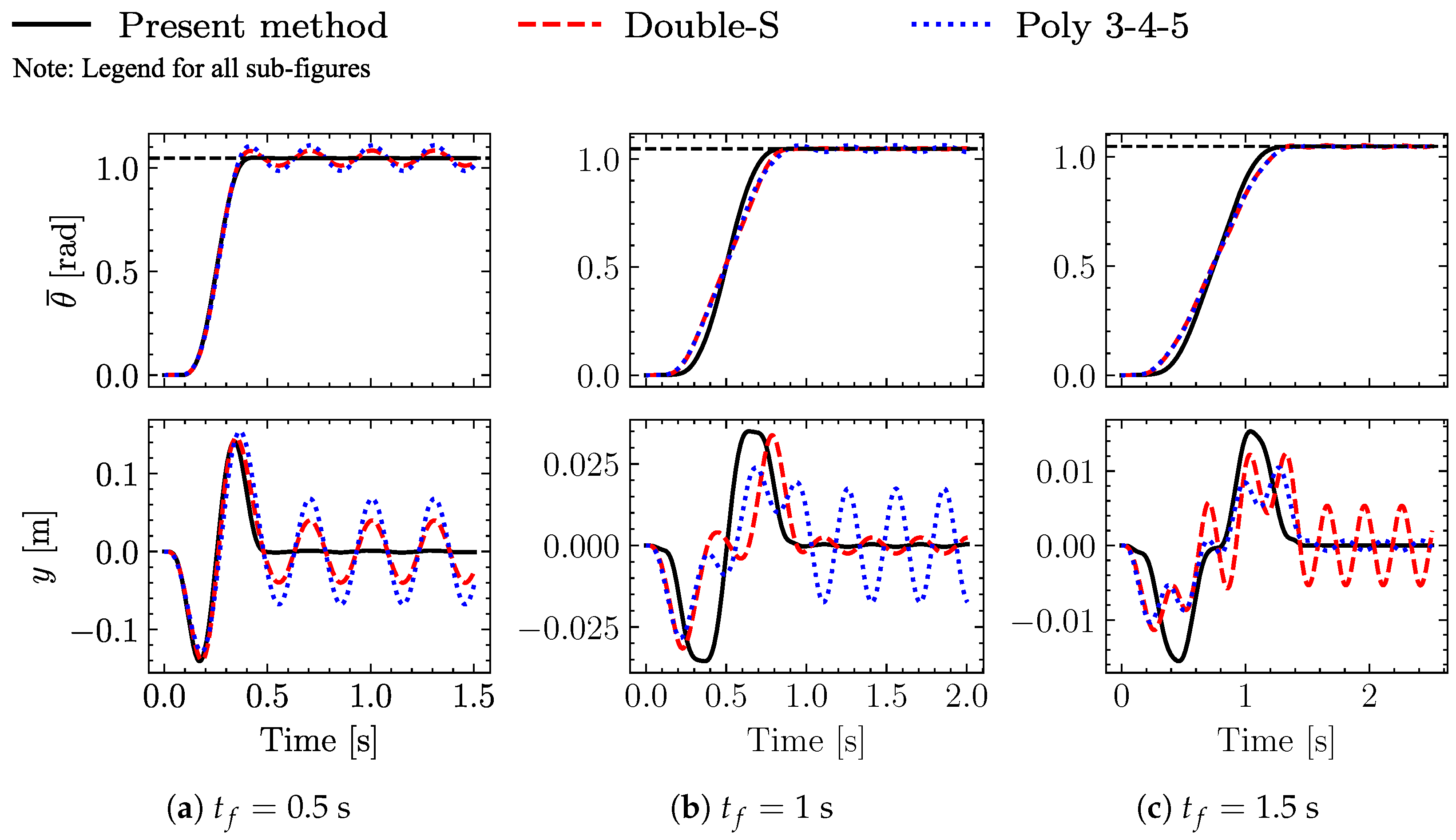
Starting with the evaluation of the motion profiles in Section 3.1, the results of the simulation are compared with those obtained by applying two common motion profiles, viz the constant-jerk double-S and the polynomial 3-4-5, [43], which are typically implemented in industrial applications.

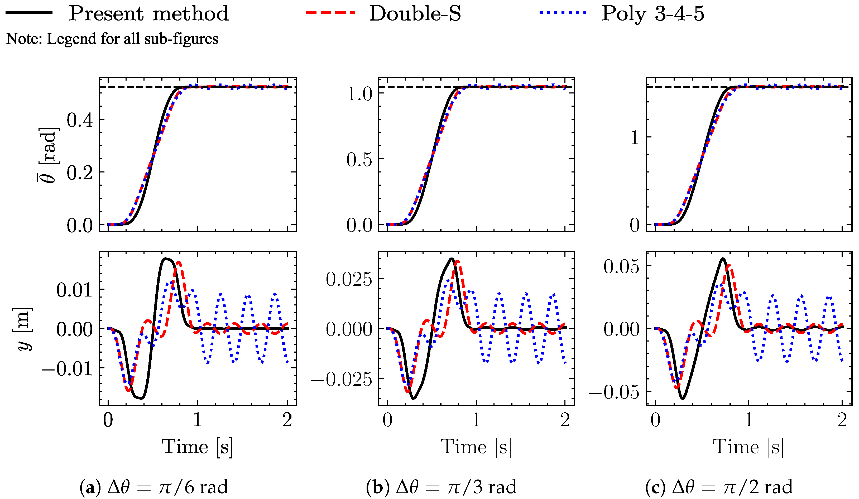
Figure 6 and Figure 7 show the results obtained for Case I and Case II (according to Table 2), respectively. For each sub-case, the system’s response is represented either as the angular displacement at the end-point of the beam $\overline{\theta }\left(t\right)$ or as the transverse deflection $y(L,t)$ with respect to the moving frame $(X,Y,Z)$ (with reference to Figure 1). The simulation results show that a significant reduction in residual vibration is achieved by the proposed method. Related quantitative data are provided in

Table 4. Performance analysis of the present method, the constant-jerk double-S and polynomial 3-4-5 motion laws for the three sub-cases of Case I detailed in Section 3.1.

Motion Law	Actuation Time	Residual Vibration	Vibration Reduction
	[s]	[mm]	[%]
Present Method	0.5	1.44	-
Poly345	0.5	67.79	97.9
Double-S	0.5	40.16	96.4
Present Method	1.0	0.40	-
Poly345	1.0	17.41	97.7
Double-S	1.0	2.47	83.8
Present Method	1.5	0.04	-
Poly345	1.5	0.70	94.3
Double-S	1.5	5.34	99.3

and

Table 5. Performance analysis of the present method, the constant-jerk double-S and polynomial 3-4-5 motion laws for the three sub-cases of Case II detailed in Section 3.1.

Motion Law	Actuation Time	Residual Vibration	Vibration Reduction
	[rad]	[mm]	[%]
Present Method	$\pi /6$	0.07	-
Poly345	$\pi /6$	8.69	99.2
Double-S	$\pi /6$	1.29	94.6
Present Method	$\pi /3$	0.60	-
Poly345	$\pi /3$	17.41	96.6
Double-S	$\pi /3$	2.47	75.7
Present Method	$\pi /2$	1.35	-
Poly345	$\pi /2$	26.17	94.8
Double-S	$\pi /2$	3.46	61.0

, where the advantages of the proposed approach over comparison methods can be clearly seen.

Figure 8 shows the results for multi-target case study reported in Section 3.2, where the transverse displacement of the beam during movement is illustrated. Once again, the significant reduction in residual vibration in the three target sections (the constant velocity sections, the rest section and the end of the movement) demonstrates the method’s effectiveness.

5. Conclusions

In this work, a new methodology to preshape the motion profile of a controlled flexible system was presented. The method aims to minimise the residual vibration by solving a QP problem subject to linear constraints, in which a function that estimates the residual vibrational energy of the system is minimised. The motion profile is described by a time-parametrised spline in its B-form, and the unknowns of the minimisation problem consist of the control points that define the control polygon of the acceleration profile. The technique proposed was applied to control the angular displacement of an Euler–Bernoulli beam in two different scenarios: rest-to-rest motion planning and multi-target applications. In the latter, vibration reduction was accomplished at several instances of the motion profile, which is concatenated using an iso-parametric approach. The model used to estimate the energy of the flexible link was a simplified linear model, in which some effects, such as centrifugal and Coriolis forces, where neglected. In this respect, the method’s effectiveness was tested including these effects in a simulated environment and using an FE model. A comparison of the results with those obtained using the motion profiles typically implemented in industrial applications is presented. The simulations, conducted using the open-source simulation engine projectchrono, showed the approach’s effectiveness in significantly minimising the vibration at the target points. The suggested approach also enabled high levels of motion smoothness while ensuring compliance with the kinematic limits given by the physical system (in the proposed application up to the jerk). Furthermore, an appealing aspect of the technique was the ease of implementation, which does not require adding new hardware to the system and allows for the easy addition of constraints to the problem, e.g., waypoint interpolation. In future work, we plan to numerically and experimentally test the method for multi-link flexible structures and to extend the approach to multi-objective cost functions and more complicated structures exploiting the Iso-Geometric Analysis method.